Knowledge-Aided Kaczmarz and LMS Algorithms

Abstract

The least mean squares (LMS) filter is often derived via the Wiener filter solution. For a system identification scenario, such a derivation makes it hard to incorporate prior information on the system’s impulse response. We present an alternative way based on the maximum a posteriori solution, which allows developing a Knowledge-Aided Kaczmarz algorithm. Based on this Knowledge-Aided Kaczmarz we formulate a Knowledge-Aided LMS filter. Both algorithms allow incorporating the prior mean and covariance matrix on the parameter to be estimated. The algorithms use this prior information in addition to the measurement information in the gradient for the iterative update of their estimates. We analyze the convergence of the algorithms and show simulation results on their performance. As expected, reliable prior information allows improving the performance of the algorithms for low signal-to-noise (SNR) scenarios. The results show that the presented algorithms can nearly achieve the optimal maximum a posteriori (MAP) performance.

I Introduction

Knowledge-Aided estimation algorithms have a long tradition in digital signal processing, with research areas ranging from generalized Bayesian estimation [1, 2] over positioning and target tracking [3, 4] to direction of arrival estimation [5, 6, 7]. However, to the best of our knowledge, there is no knowledge-aided least mean squares (LMS) filter described in literature, allowing to incorporate prior information on the filter coefficients to be estimated.

For the LMS filter, a standard way for derivation is based on the Wiener filter solution [8, 9, 10, 11, 12]. The Wiener filter can be seen as a Bayesian estimator utilizing statistical information on its input $x[k]$, as well as statistical information on the relation of its input to a desired output signal $y[k]$. Its aim is to minimize the mean square error (MSE) between the filter output and the desired output signal, leading to the famous Wiener solution [13, 14], for the optimal filter coefficients ${\mathbf{\bm{\thetaup}}}_{\text{opt}}$:

$${\mathbf{\bm{\thetaup}}}_{\text{opt}}={\mathbf{R}}_{xx}^{-1}{\mathbf{r}}_{xy}$$ (1)

with ${\mathbf{R}}_{xx}$ as the autocorrelation matrix of the input and ${\mathbf{r}}_{xy}$ as the cross-correlation vector between the input of the Wiener filter and the desired output signal. An LMS adaptive filter can be seen as a method implicitly approximating ${\mathbf{R}}_{xx}$ and ${\mathbf{r}}_{xy}$ using instantaneous estimates [11]. A prominent applications scenario for adaptive filters is system identification [15].

Here the aim is not to optimally estimate the output of the filter but to optimally estimate an unknown system with impulse response ${\mathbf{\bm{\thetaup}}}$.

When considering this scenario, a Wiener filter approach makes it hard to incorporate prior knowledge on ${\mathbf{\bm{\thetaup}}}$. As an alternative that allows to incorporate such a prior knowledge, we suggest the following way to derive the LMS filter. We first start with a batch based approach and develop a Knowledge-Aided Kaczmarz algorithm. Then we extend the Kaczmarz algorithm to an LMS filter. This extension can be easily done due to the arithmetic similarity of the Kaczmarz algorithm and the LMS filter when using the Kaczmarz algorithm with a convolution matrix.

Emphasizing its versatility, the presented approach is based on a general linear model that has a widespread application potential:

$${\mathbf{y}}={\mathbf{H}}{\mathbf{\bm{\thetaup}}}+{\mathbf{n}}.$$ (2)

The dimensions of ${\mathbf{H}}$ are $m\times p$, of $\mathbf{\bm{\thetaup}}$ are $p\times 1$ and of $\mathbf{n}$ and $\mathbf{y}$ are $m\times 1$, respectively. The rows of ${\mathbf{H}}$ will be denoted as ${\mathbf{h}}_{i}^{T}$ and the elements of $\mathbf{y}$ and $\mathbf{n}$ as $y_{i}$ as well as $n_{i}$, $\forall i=1,\ldots,m$, respectively. In the general case, ${\mathbf{H}}$ will be an arbitrary system or observation matrix, which we assume to have full rank. For the case of an LMS filter, ${\mathbf{H}}$ will be a convolution matrix with potentially an unlimited number of rows. The vector ${\mathbf{y}}$ is the measurement vector. The parameter vector ${\mathbf{\bm{\thetaup}}}$ is assumed to be a Gaussian random variable with mean $\bar{\mathbf{\bm{\thetaup}}}$ and covariance matrix ${\mathbf{C}}_{{\mathbf{\bm{\thetaup}}}{\mathbf{\bm{\thetaup}}}}$. These statistics of ${\mathbf{\bm{\thetaup}}}$ will be used as prior information in the estimation algorithms described below. The noise vector $\mathbf{n}$ is assumed to be Gaussian as well, with zero mean and covariance matrix ${\mathbf{C}}_{\mathbf{n}\mathbf{n}}$. In the following derivation, we will assume that ${\mathbf{C}}_{\mathbf{n}\mathbf{n}}$ is a diagonal matrix. We furthermore assume that ${\mathbf{C}}_{\mathbf{\bm{\thetaup}}\mathbf{\bm{\thetaup}}}$ is positive definite, which can always be ensured by adding a scaled identity matrix $\sigma\mathbf{I}$, using a small positive scaling factor $\sigma$.

This work can somehow be seen as being related to the approach in [16]. There, prior information is used on the model to incorporate systems with missing data. Different to that, we incorporate prior knowledge on the parameter vector to be estimated. Another connection might be drawn to [17], where the author uses a different cost function as we do, incorporating previous estimates of the LMS algorithm. Its applications as well as the resulting algorithms are different to our approach. Another different approach is used in the Generalized Sidelobe Canceler version of the LMS. There the input signal is altered by a so-called Blocking Matrix to improve the estimation performance[18].

II Knowledge-Aided Kaczmarz algorithm

In this section, we will derive the Knowledge-Aided Kaczmarz algorithm incorporating the prior information on $\mathbf{\bm{\thetaup}}$. The idea is to develop an iterative steepest descent approach similar to Approximate Least Squares (ALS) [19] or the Kaczmarz algorithm [20]. For this, we start with a maximum a posterior (MAP) approach.

The derivation of the MAP estimator for the model in (2) results in an estimator of the same form as the linear minimum mean square error (LMMSE) estimator [21]. This naturally allows using our algorithms for other use cases of the LMMSE estimator as well. The Knowledge-Aided Kaczmarz algorithm developed in this chapter can be seen as an iterative variant of the batch LMMSE estimator, while the Knowledge-Aided LMS developed below can be seen as an LMS variant of an LMMSE estimator using a convolution matrix.

II-A Derivation via the MAP solution

The posterior probability can be calculated as

$$p({\mathbf{\bm{\thetaup}}}|{\mathbf{y}})=p({\mathbf{y}}|{\mathbf{\bm{\thetaup}}})p({\mathbf{\bm{\thetaup}}})/p({\mathbf{y}})\propto p({\mathbf{y}}|{\mathbf{\bm{\thetaup}}})p({\mathbf{\bm{\thetaup}}}).$$ (3)

The MAP estimate is the vector

$$\hat{\mathbf{\bm{\thetaup}}}_{\text{MAP}}=\underset{{\mathbf{\bm{\thetaup}}}}{\text{arg max }}p({\mathbf{y}}|{\mathbf{\bm{\thetaup}}})p({\mathbf{\bm{\thetaup}}}).$$ (4)

Here we use $\hat{\mathbf{\bm{\thetaup}}}$ to represent an estimate of a true parameter vector ${\mathbf{\bm{\thetaup}}}_{T}$. Taking the logarithm and omitting the Gaussian scaling factors gives:

$$\hat{\mathbf{\bm{\thetaup}}}_{\text{MAP}}=\underset{{\mathbf{\bm{\thetaup}}}}{\text{ arg max }} \text{log }p({\mathbf{y}}|{\mathbf{\bm{\thetaup}}})p({\mathbf{\bm{\thetaup}}})$$ (5)

$$=\underset{{\mathbf{\bm{\thetaup}}}}{\text{ arg max }} -({\mathbf{y}}-{\mathbf{H}}{\mathbf{\bm{\thetaup}}})^{T}{\mathbf{C}}_{\mathbf{n}\mathbf{n}}^{-1}({\mathbf{y}}-{\mathbf{H}}{\mathbf{\bm{\thetaup}}})$$

$$-({\mathbf{\bm{\thetaup}}}-\bar{\mathbf{\bm{\thetaup}}})^{T}{\mathbf{C}}_{\mathbf{\bm{\thetaup}}\mathbf{\bm{\thetaup}}}^{-1}({\mathbf{\bm{\thetaup}}}-\bar{\mathbf{\bm{\thetaup}}})$$ (6)

Multiplying the cost function with $-1$ leads to the optimization problem

$$\hat{\mathbf{\bm{\thetaup}}}_{\text{MAP}} =\underset{{\mathbf{\bm{\thetaup}}}}{\text{arg min }}J({\mathbf{\bm{\thetaup}}})$$ (7)

with ${J({\mathbf{\bm{\thetaup}}})=({\mathbf{y}}-{\mathbf{H}}{\mathbf{\bm{\thetaup}}})^{T}{\mathbf{C}}_{\mathbf{n}\mathbf{n}}^{-1}({\mathbf{y}}-{\mathbf{H}}{\mathbf{\bm{\thetaup}}})+({\mathbf{\bm{\thetaup}}}-\bar{\mathbf{\bm{\thetaup}}})^{T}{\mathbf{C}}_{\mathbf{\bm{\thetaup}}\mathbf{\bm{\thetaup}}}^{-1}({\mathbf{\bm{\thetaup}}}-\bar{\mathbf{\bm{\thetaup}}})}$.

This cost function can be split into two parts, a first part $({\mathbf{y}}-{\mathbf{H}}{\mathbf{\bm{\thetaup}}})^{T}{\mathbf{C}}_{\mathbf{n}\mathbf{n}}^{-1}({\mathbf{y}}-{\mathbf{H}}{\mathbf{\bm{\thetaup}}})$ that we will call measurement cost function and a second part $({\mathbf{\bm{\thetaup}}}-\bar{\mathbf{\bm{\thetaup}}}){\mathbf{C}}_{\mathbf{\bm{\thetaup}}\mathbf{\bm{\thetaup}}}^{-1}({\mathbf{\bm{\thetaup}}}-\bar{\mathbf{\bm{\thetaup}}})$ that we will call prior cost function. Calculating the partial derivative of $J({\mathbf{\bm{\thetaup}}})$ results in

$$\nabla({\mathbf{\bm{\thetaup}}})=\frac{\partial J({\mathbf{\bm{\thetaup}}})}{\partial{\mathbf{\bm{\thetaup}}}}=2{\mathbf{H}}^{T}{\mathbf{C}}_{\mathbf{n}\mathbf{n}}^{-1}({\mathbf{H}}{\mathbf{\bm{\thetaup}}}-{\mathbf{y}})+2{\mathbf{C}}_{\mathbf{\bm{\thetaup}}\mathbf{\bm{\thetaup}}}^{-1}({\mathbf{\bm{\thetaup}}}-\bar{\mathbf{\bm{\thetaup}}}).$$ (8)

This gradient can be used to formulate a steepest descent approach as

$$\hat{\mathbf{\bm{\thetaup}}}^{(k)}= \;\hat{\mathbf{\bm{\thetaup}}}^{(k-1)}-\mu\nabla({\hat{\mathbf{\bm{\thetaup}}}^{(k-1)}})$$ (9)

$$= \;\hat{\mathbf{\bm{\thetaup}}}^{(k-1)}-\mu\left({\mathbf{H}}^{T}{\mathbf{C}}_{\mathbf{n}\mathbf{n}}^{-1}({\mathbf{H}}\hat{\mathbf{\bm{\thetaup}}}^{(k-1)}-{\mathbf{y}})\right.$$

$$\left.+{\mathbf{C}}_{\mathbf{\bm{\thetaup}}\mathbf{\bm{\thetaup}}}^{-1}(\hat{\mathbf{\bm{\thetaup}}}^{(k-1)}-\bar{\mathbf{\bm{\thetaup}}})\right),$$ (10)

with the step width $\mu$. For simplicity, we omitted the factor two of the gradient and assumed that this factor is already included in the step width. An iteration can be formulated via a sum of partial gradients ${\mathbf{h}_{i}}w_{i}({\mathbf{h}_{i}}^{T}\hat{\mathbf{\bm{\thetaup}}}^{(k-1)}-{y_{i}})+a_{i}\;{\mathbf{C}}_{\mathbf{\bm{\thetaup}}\mathbf{\bm{\thetaup}}}^{-1}(\hat{\mathbf{\bm{\thetaup}}}^{(k-1)}-\bar{\mathbf{\bm{\thetaup}}})$:

$$\hat{\mathbf{\bm{\thetaup}}}^{(k)}=\hat{\mathbf{\bm{\thetaup}}}^{(k-1)}-\mu\sum_{i=1}^{m} \left({\mathbf{h}_{i}}w_{i}({\mathbf{h}_{i}}^{T}\hat{\mathbf{\bm{\thetaup}}}^{(k-1)}-{y_{i}})\right.$$

$$+\left.a_{i}\;{\mathbf{C}}_{\mathbf{\bm{\thetaup}}\mathbf{\bm{\thetaup}}}^{-1}(\hat{\mathbf{\bm{\thetaup}}}^{(k-1)}-\bar{\mathbf{\bm{\thetaup}}})\right),$$ (11)

with $w_{i}$ as the $(i,i)^{th}$ element of ${\mathbf{C}}_{\mathbf{n}\mathbf{n}}^{-1}$. The values $a_{i}$ are used to bring the gradient of the prior cost function inside the sum, requiring that $\sum_{i=1}^{m}a_{i}=1$. We will furthermore assume that $a_{i}>0,\;\forall i=1,\ldots,m$. One obvious way of fulfilling this condition on the $a_{i}$ values is by setting $a_{i}=1/m,\;\forall i=1,\ldots,m$. The cost function as well as its gradients are schematically depicted in Fig. 1.

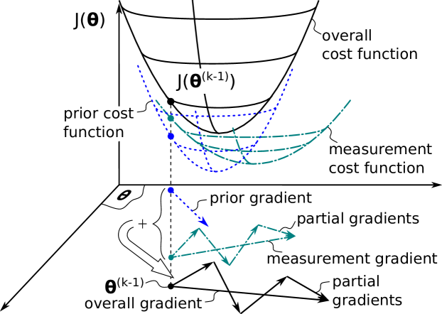
Figure 1: Cost functions and gradients.

As one can see in this figure, the gradient of the prior cost function redirects the gradient of the measurement cost function. This allows utilizing the prior information in the gradient based algorithm, improving its performance, as we will show below.

The above formulation easily allows to use simplifications as done in the ALS [19] or the Kaczmarz algorithm [20], by using only one of the partial gradients per iteration and cyclically re-using the partial gradients after $m$ iterations:

$$\hat{\mathbf{\bm{\thetaup}}}^{(k)}=\hat{\mathbf{\bm{\thetaup}}}^{(k-1)}-\mu_{k} \left({\mathbf{h}_{k\urcorner}}w_{k\urcorner}({\mathbf{h}_{k\urcorner}}^{T}\hat{\mathbf{\bm{\thetaup}}}^{(k-1)}-{y_{k\urcorner}})\right.$$

$$+\left.a_{k\urcorner}\;{\mathbf{C}}_{\mathbf{\bm{\thetaup}}\mathbf{\bm{\thetaup}}}^{-1}(\hat{\mathbf{\bm{\thetaup}}}^{(k-1)}-\bar{\mathbf{\bm{\thetaup}}})\right).$$ (12)

Here, $k\urcorner=((k-1)\text{ mod }m)+1$, represents this cyclic re-use. $\mu_{k}$ is the (not necessarily constant) step width used in iteration $k$. We will describe how to select this step width in more detail in the next section. When using $a_{k\urcorner}=1/m$, ${\forall{k\urcorner}=1,\ldots,m}$, one can see a Bayesian-like characteristic in the partial gradients. The prior information is scaled by one over the number of samples: the more data is collected, the less important the prior information becomes. We call the iterative approach using (12): Knowledge-Aided Kaczmarz.

II-B Convergence of Knowledge-Aided Kaczmarz

Using the iteration (12) of Knowledge-Aided Kaczmarz one can analyze the evolution of the error ${\mathbf{e}}^{(k)}=\hat{\mathbf{\bm{\thetaup}}}^{(k)}-{\mathbf{\bm{\thetaup}}}_{T}$ comparing an estimate $\hat{\mathbf{\bm{\thetaup}}}^{(k)}$ at iteration $k$ to the true parameter vector $\mathbf{\bm{\thetaup}}_{T}$. Inserting this error in (12) and using $y_{k\urcorner}={\mathbf{h}}_{k\urcorner}^{T}{\mathbf{\bm{\thetaup}}}_{T}+n_{k\urcorner}$ gives

$${\mathbf{e}}^{(k)}={\mathbf{M}}_{k\urcorner}{\mathbf{e}}^{(k-1)}+\mu_{k}{\mathbf{h}}_{k\urcorner}w_{k\urcorner}n_{k\urcorner}+\mu_{k}a_{k\urcorner}\;{\mathbf{C}}_{\mathbf{\bm{\thetaup}}\mathbf{\bm{\thetaup}}}^{-1}({\mathbf{\bm{\thetaup}}}_{T}-\bar{\mathbf{\bm{\thetaup}}}),$$

with ${\mathbf{M}}_{k\urcorner}=\left({\mathbf{I}}-\mu_{k}\left({\mathbf{h}}_{k\urcorner}w_{k\urcorner}{\mathbf{h}}_{k\urcorner}^{T}+a_{k\urcorner}\;{\mathbf{C}}_{\mathbf{\bm{\thetaup}}\mathbf{\bm{\thetaup}}}^{-1}\right)\right)$. The matrix ${\mathbf{P}}_{k\urcorner}=\left({\mathbf{h}}_{k\urcorner}w_{k\urcorner}{\mathbf{h}}_{k\urcorner}^{T}+a_{k\urcorner}\;{\mathbf{C}}_{\mathbf{\bm{\thetaup}}\mathbf{\bm{\thetaup}}}^{-1}\right)$ consists of a sum of a symmetric and positive semidefinite matrix and a symmetric and positive definite matrix. The matrix ${\mathbf{h}}_{k\urcorner}w_{k\urcorner}{\mathbf{h}}_{k\urcorner}^{T}$ has $p-1$ eigenvalues that are zero and one eigenvalue that is equal to $w_{k\urcorner}\|{\mathbf{h}}_{k\urcorner}\|_{2}^{2}$, corresponding to the eigenvector ${\mathbf{h}}_{k\urcorner}$. ${\mathbf{C}}_{\mathbf{\bm{\thetaup}}\mathbf{\bm{\thetaup}}}$ is a covariance matrix that we assumed to be positive definite, as described in the introduction of this paper. For such a sum of matrices one can easily find limits on its eigenvalues. For this we define the sequence $\lambda_{i}(\mathbf{A}),\forall i=1,\ldots,p$, as the eigenvalues of a $p\times p$ matrix $\mathbf{A}$ in descending order, i.e. $\lambda_{1}(\mathbf{A})$ being the largest eigenvalue, down to $\lambda_{p}(\mathbf{A})$ being the smallest eigenvalue.

For two symmetric $p\times p$ matrices $\mathbf{A}$ and $\mathbf{B}$ it holds that the maximum eigenvalue of the sum of matrices, $\lambda_{1}(\mathbf{A}+\mathbf{B})$ is smaller or equal than the sum of the maximum eigenvalues of the matrices [22]:

$$\lambda_{1}(\mathbf{A}+\mathbf{B})\leq\lambda_{1}(\mathbf{A})+\lambda_{1}(\mathbf{B}).$$ (13)

Because we assumed ${\mathbf{C}}_{\mathbf{\bm{\thetaup}}\mathbf{\bm{\thetaup}}}$ to be positive definite and due to Weyl’s inequality [22, 23]

$$\lambda_{i}(\mathbf{A})+\lambda_{p}(\mathbf{B})\leq\lambda_{i}(\mathbf{A}+\mathbf{B})\leq\lambda_{i}(\mathbf{A})+\lambda_{1}(\mathbf{B}),$$ (14)

$\forall i=1,\ldots,p$, it immediately follows that the smallest eigenvalue of ${\mathbf{P}}_{k\urcorner}$ must be larger than zero. The aforementioned relations on the eigenvalues can be used to define an interval for $\mu_{k}$ limiting the eigenvalues of ${\mathbf{M}}_{k\urcorner}$. Using

$$0<\mu_{k}\leq\frac{1}{w_{k\urcorner}||h_{k\urcorner}||_{2}^{2}+a_{k\urcorner}\lambda_{1}({\mathbf{C}}_{\mathbf{\bm{\thetaup}}\mathbf{\bm{\thetaup}}}^{-1})}$$ (15)

ensures that all eigenvalues of $\mu_{k}{\mathbf{P}}_{k\urcorner}$ are smaller or equal than one and larger than zero. Consequently, all eigenvalues of ${\mathbf{M}}_{k\urcorner}$ are smaller than one and larger or equal to zero for all ${{k\urcorner}=1,\ldots,p}$. When partitioning (II-B) into

$${\mathbf{e}}^{(k)}=\prod_{i=1}^{k}{\mathbf{M}}_{i\urcorner}{\mathbf{e}}^{(0)}+{\mathbf{\Delta}}_{k}+\sum_{i=1}^{k-1}\left(\prod_{j=i+1}^{k}{\mathbf{M}}_{j\urcorner}\right){\mathbf{\Delta}}_{i},$$ (16)

with ${\mathbf{\Delta}}_{k}=\mu_{k}\left({\mathbf{h}}_{k\urcorner}w_{k\urcorner}n_{k\urcorner}+a_{k\urcorner}\;{\mathbf{C}}_{\mathbf{\bm{\thetaup}}\mathbf{\bm{\thetaup}}}^{-1}({\mathbf{\bm{\thetaup}}}-\bar{\mathbf{\bm{\thetaup}}})\right)$, we can analyze the error evolution for $k\rightarrow\infty$. We denote this error as ${\mathbf{e}}^{(\infty)}$.

The initial error vector ${\mathbf{e}}^{(0)}$ is caused by the start vector $\mathbf{\bm{\thetaup}}^{(0)}$ of the Kaczmarz iterations. When choosing $\mu_{k}$ according to (15), the first product $\prod_{i=1}^{k}{\mathbf{M}}_{i\urcorner}{\mathbf{e}}^{(0)}$ converges to the zero vector because all eigenvalues of every ${\mathbf{M}}_{i\urcorner}$ are smaller than one, as long as $\mu$ is within the bounds of 15. Additionally there are the noise and bias dependent residual terms ${\mathbf{\Delta}}_{k}$. Because ${\mathbf{\Delta}}_{k}$ is linear in $\mu$, the error ${\mathbf{e}}^{(\infty)}$ can be made arbitrary small by selecting a small enough (but larger than zero) value of $\mu$.

However, when analyzing the expected value of ${\mathbf{e}}^{(\infty)}$ averaged over $\mathbf{n}$ as well as over $\mathbf{\bm{\thetaup}}$ one can see that this expected value is zero:

$$E_{\mathbf{n},\mathbf{\bm{\thetaup}}}({\mathbf{e}}^{(\infty)})= E_{\mathbf{n},\mathbf{\bm{\thetaup}}}({\mathbf{\Delta}}_{k})+\sum_{i=1}^{k-1}\left(\prod_{j=i+1}^{k}{\mathbf{M}}_{j\urcorner}\right)E_{\mathbf{n},\mathbf{\bm{\thetaup}}}({\mathbf{\Delta}}_{i})=\mathbf{0}$$ (17)

This shows that the Knowledge-Aided Kaczmarz converges in the mean.

Using the limits on $\mu_{k}$ as described above, we formulate the following Algorithm 1 that we used for the simulation results presented below.

Algorithm 1 Knowledge-Aided Kaczmarz

1:precalculate ${\mathbf{C}}_{\mathbf{\bm{\thetaup}}\mathbf{\bm{\thetaup}}}^{-1}$, $\lambda_{1}({\mathbf{C}}_{\mathbf{\bm{\thetaup}}\mathbf{\bm{\thetaup}}}^{-1})$

2:$\hat{\mathbf{\bm{\thetaup}}}^{(0)}\leftarrow{\bf 0}$ , $v_{k}\leftarrow 0$, $v_{k-m}\leftarrow\{\text{largest available number}\}$

3:ReduceMu $\leftarrow$ False

4:for $k=1,\ldots,N$ do

5:    $v_{k}\leftarrow{y_{k\urcorner}}-{\bf h}_{k\urcorner}^{T}\hat{\mathbf{\bm{\thetaup}}}^{(k-1)}$

6:    if ReduceMu then

7:         $\mu_{k}\leftarrow\mu_{k-1}-\mu_{r}$

8:    else

9:         $\mu_{k}\leftarrow\frac{1}{w_{k\urcorner}||h_{k\urcorner}||_{2}^{2}+a_{k\urcorner}\lambda_{1}({\mathbf{C}}_{\mathbf{\bm{\thetaup}}\mathbf{\bm{\thetaup}}}^{-1})}$

10:         if $k\urcorner=1$ then

11:             if $|v_{k}-v_{k-m}|<v_{th}$ then

12:                 ReduceMu $\leftarrow$ True

13:                 $\mu_{k}\leftarrow\frac{1}{\underset{i=1,\ldots,m}{\text{max }}({w_{i}||h_{i}||_{2}^{2}+a_{k\urcorner}\lambda_{1}({\mathbf{C}}_{\mathbf{\bm{\thetaup}}\mathbf{\bm{\thetaup}}}^{-1})})}$

14:                 $\mu_{r}=\mu_{k}/(N-k+1)$

15:             end if

16:             $v_{k-m}\leftarrow v_{k}$

17:         end if

18:    end if

19:    $\hat{\mathbf{\bm{\thetaup}}}^{(k)}\leftarrow\hat{\mathbf{\bm{\thetaup}}}^{(k-1)}+\mu_{k}\left({\bf h}_{k\urcorner}w_{k\urcorner}v_{k}+a_{k\urcorner}{\mathbf{C}}_{\mathbf{\bm{\thetaup}}\mathbf{\bm{\thetaup}}}^{-1}(\hat{\mathbf{\bm{\thetaup}}}^{(k-1)}-\bar{\mathbf{\bm{\thetaup}}})\right)$

20:end for

In the beginning, the algorithm uses the upper limits of the interval in (15) as step widths. For a practical implementation, one would typically pre-calculate these $m$ values and store them in a memory. From the iteration where the instantaneous error $v_{k}$ differs less than $v_{th}$ to the error $m$ iterations before, the step width is linearly reduced down to zero with every following iteration. For simplicity, $v_{k}$ and $v_{k-m}$ are only compared at iterations when the first row of $\mathbf{H}$ and the first measurement value from $\mathbf{y}$ are used. Such a step width reduction typically leads to a very good performance for Kaczmarz-like algorithms [24].

As pointed out above, for the model (2) the MAP solution is identical to the LMMSE solution. This means LMMSE algorithms, such as the sequential LMMSE [21], could also be used. However when analyzing the complexity of LMMSE approaches, e.g. as done in [25], one can see that the complexity of such approaches is typically $\mathcal{O}(p^{3})$. For the Knowledge-Aided Kaczmarz algorithm, the complexity per iteration depends on the matrix ${\mathbf{C}}_{\mathbf{\bm{\thetaup}}\mathbf{\bm{\thetaup}}}$. If ${\mathbf{C}}_{\mathbf{\bm{\thetaup}}\mathbf{\bm{\thetaup}}}$ is a full matrix, the complexity per iteration is $\mathcal{O}(p^{2})$, if ${\mathbf{C}}_{\mathbf{\bm{\thetaup}}\mathbf{\bm{\thetaup}}}$ is a diagonal matrix, Knowledge-Aided Kaczmarz only has linear complexity per iteration.

III Knowledge-Aided LMS Filter

The Knowledge-Aided Kaczmarz algorithm can be easily extended to a Knowledge-Aided LMS filter. For an LMS filter, $\mathbf{H}$ has the structure of a convolution matrix, and its number of rows $m$ is potentially unlimited. This typically prevents cyclic re-using of the rows of $\mathbf{H}$ as well as the measurement values. Equation (11) then potentially requires an infinite series $\sum_{i=1}^{\infty}a_{i}=1$. Using the same notation as above, the memory of the adaptive filter now becomes the vector $\mathbf{h}_{k}$ and the estimated filter coefficients are $\hat{\mathbf{\bm{\thetaup}}}^{(k)}$, resulting in the Knowledge-Aided LMS update equation:

$$\hat{\mathbf{\bm{\thetaup}}}^{(k)} =\hat{\mathbf{\bm{\thetaup}}}^{(k-1)}$$

$$-\mu_{k}\left({\mathbf{h}_{k}}w_{k}({\mathbf{h}_{k}}^{T}\hat{\mathbf{\bm{\thetaup}}}^{(k-1)}-{y_{k}})+a_{k}\;{\mathbf{C}}_{\mathbf{\bm{\thetaup}}\mathbf{\bm{\thetaup}}}^{-1}(\hat{\mathbf{\bm{\thetaup}}}^{(k-1)}-\bar{\mathbf{\bm{\thetaup}}})\right).$$

Using similar arguments as for the Knowledge-Aided Kaczmarz algorithm, one can see that this algorithm converges in the mean as well. This allows formulating an algorithm similar to Algorithm 1 with the exception that no cyclic re-use of rows is performed because for an LMS filter typically the number of rows of the convolution matrix $\mathbf{H}$ is equal to the number of iterations. For simplicity, we also omitted the step-width reduction logic, line 6–18 of Algorithm 1, for the LMS filter and reduced $\mu_{k}$ at every iteration by mulitipling it with $(N-k+1)/N$.

IV Simulation Results

In this section, we show simulation results for the Knowledge-Aided Kaczmarz algorithm as well as for the Knowledge-Aided LMS filter. For the shown simulations, we always used $\mathbf{C}_{\mathbf{\bm{\thetaup}}\mathbf{\bm{\thetaup}}}=0.1\mathbf{I}$ and a zero mean vector of the parameter that was to be estimated. For the Knowledge-Aided Kaczmarz algorithm, we show simulation results for $\mathbf{H}$ matrices of dimension $50\times 5$ using $500$ algorithm iterations. The entries of $\mathbf{H}$ have been selected uniformly at random from $[0,1]$. The obtained results have been averaged over $100000$ simulations. Fig. 2(a) shows the averaged error norm (over all simulations) at every iteration of the Knowledge-Aided Kaczmarz algorithm for an SNR=$0$dB. We also included the simulated MSE performance of the least squares (LS) solution as performance bound for the Kaczmarz algorithm (using the same step width reduction strategy as in Alg. 1) as well as the MSE of the MAP solution as performance bound for the Knowledge-Aided Kaczmarz algorithm. For the step width reduction of Algorithm 1, $v_{th}$ was set to $10^{-4}$ in all Kaczmarz simulations.

(a) Performance over iterations at SNR = $0$dB.

(b) Performance over SNR.

Figure 2: Simulated MSE of Knowledge-Aided Kaczmarz

As one can see from this figure, the Knowledge-Aided Kaczmarz algorithm is able to utilize the prior information, significantly reducing the final error. Due to the step width reduction, the Knowledge-Aided Kaczmarz is able to come close to the MAP performance even with as little as $500$ iterations. Fig. 2(b) shows the final simulated MSE over different SNR values. As one can see in this picture, the Knowledge Aided Kaczmarz algorithm comes close to the MAP solution for all SNR values. As expected, the prior information significantly increases the performance especially at low SNR values.

Fig. 4 shows the simulation results for the Knowledge-Aided LMS filter. Here, we again used $50$ measurement values, resulting in $m=50$ iterations for the LMS filters. We estimated a system impulse response of length $5$ in a system identification scenario. The input of the LMS filters as well as the unknown systems have been selected uniformly at random from $[0,1]$. We used $a_{i}=1/m,\;\forall i=1,\ldots,m$, for these simulations. Fig. 3(a) shows the simulated MSE over the iterations $k$ for SNR=$-2$dB. As one can see, the prior information significantly improves the performance of the Knowledge-Aided LMS filter as well.

(a) Performance over iterations at SNR = $-2$dB.

(b) Performance over SNR.

Figure 3: Simulated MSE of Knowledge-Aided LMS filter.

Fig. 3(b) shows simulated MSE results after 50 iterations of the LMS filter as well as the Knowledge-Aided LMS filter over different SNR values. Again, as expected, the major gains are at low SNR values, if reliable prior information is present. Fig. 3(a) also allows to describe the performance of the Knowledge-Aided LMS from another point of view: is able to achieve a fixed performance level with a lower number of measurements than the conventional LMS filter.

V Conclusion

We presented Knowledge-Aided Kaczmarz and Knowledge-Aided LMS algorithms that easily allow utilizing prior information to improve the performance of the algorithms. We derived the algorithms via the maximum a posteriori solution. Their convergence behavior was analyzed, and it was shown that both algorithms converge in the mean. For low SNR scenarios, the Knowledge-Aided algorithms significantly outperform the standard algorithms. The simulations furthermore show that the Knowledge-Aided algorithms are able to achieve a performance close to the MAP performance.

References

- [1] O. Besson, N. Dobigeon, and J. Y. Tourneret, “Joint Bayesian Estimation of Close Subspaces from Noisy Measurements,” In IEEE Signal Processing Letters, Vol. 21, No. 2, pp. 168–171, Feb 2014.
- [2] A. Amini, U. S. Kamilov, E. Bostan, and M. Unser, “Bayesian Estimation for Continuous-Time Sparse Stochastic Processes,” In IEEE Transactions on Signal Processing, Vol. 61, No. 4, pp. 907–920, Feb 2013.
- [3] J. G. Garcia, P. A. Roncagliolo, and C. H. Muravchik, “A Bayesian Technique for Real and Integer Parameters Estimation in Linear Models and Its Application to GNSS High Precision Positioning,” In IEEE Transactions on Signal Processing, Vol. 64, No. 4, pp. 923–933, Feb 2016.
- [4] A. Turlapaty and Y. Jin, “Bayesian Sequential Parameter Estimation by Cognitive Radar With Multiantenna Arrays,” In IEEE Transactions on Signal Processing, Vol. 63, No. 4, pp. 974–987, Feb 2015.
- [5] S. F. B. Pinto and R. C. d. Lamare, “Two-Step Knowledge-Aided Iterative ESPRIT Algorithm,” In WSA 2017; 21th International ITG Workshop on Smart Antennas, pp. 1–5, March 2017.
- [6] Z. Yang, R. C. de Lamare, X. Li, and H. Wang, “Knowledge-Aided STAP Using Low Rank and Geometry Properties,” In International Journal of Antennas and Propagation, pp. 1–14, Aug 2014.
- [7] X. Zhu, J. Li, and P. Stoica, “Knowledge-aided adaptive beamforming,” In IET Signal Processing, Vol. 2, No. 4, pp. 335–345, December 2008.
- [8] B. Widrow, J. M. McCool, M. G. Larimore, and C. R. Johnson, “Stationary and nonstationary learning characteristics of the LMS adaptive filter,” In Proceedings of the IEEE, Vol. 64, No. 8, pp. 1151–1162, Aug 1976.
- [9] L. Horowitz and K. Senne, “Performance advantage of complex LMS for controlling narrow-band adaptive arrays,” In IEEE Transactions on Acoustics, Speech, and Signal Processing, Vol. 29, No. 3, pp. 722–736, Jun 1981.
- [10] A. Feuer and E. Weinstein, “Convergence analysis of LMS filters with uncorrelated Gaussian data,” In IEEE Transactions on Acoustics, Speech, and Signal Processing, Vol. 33, No. 1, pp. 222–230, Feb 1985.
- [11] S. Haykin, Adaptive Filter Theory, 4th ed. Upper Saddle River, NJ: Prentice Hall, 2002.
- [12] M. Rupp, “The LMS algorithm under arbitrary linearly filtered processes,” In 19th European Signal Processing Conference, pp. 126–130, Aug 2011.
- [13] N. Wiener, Extrapolation, Interpolation, and Smoothing of Stationary Time Series. New York NY: Wiley, 1949.
- [14] R. G. Brown and P. Y. C. Hwang, Introduction to Random Signals and Applied Kalman Filtering. With MATLAB exercises and solutions, 3rd ed. New York NY: Wiley, 1996.
- [15] D. G. Manolakis, V. K. Ingle, and S. M. Kogon, Statistical and Adaptive Signal Processing. Norwood, MA: ARTECH HOUSE, 2005.
- [16] A. Ma and D. Needell, “Adapted Stochastic Gradient Descent for Linear Systems with Missing Data,” No. 12, p. 20p, Feb 2017. [Online]. Available: https://arxiv.org/abs/1702.07098
- [17] G. Deng, “Partial update and sparse adaptive filters,” In IET Signal Processing, Vol. 1, No. 1, pp. 9–17, March 2007.
- [18] R. K. Miranda, J. P. C. da Costa, and F. Antreich, “High accuracy and low complexity adaptive Generalized Sidelobe Cancelers for colored noise scenarios,” In Digital Signal Processing, Vol. 34, pp. 48–55, 2014.
- [19] M. Lunglmayr, C. Unterrieder, and M. Huemer, “Approximate Least Squares,” In IEEE International Conference on Acoustics, Speech and Signal Processing (ICASSP), pp. 4678–4682, May 2014.
- [20] S. Kaczmarz, “Przyblizone rozwiazywanie ukladów równan liniowych. – Angenäherte Auflösung von Systemen linearer Gleichungen.” In Bulletin International de l’Académie Polonaise des Sciences et des Lettres. Classe des Sciences Mathématiques et Naturelles. Série A, Sciences Mathématiques, Vol. 35, pp. 355–357, 1937.
- [21] S. M. Kay, Fundamentals of Statistical Signal Processing: Estimation Theory. Prentice Hall, 1997.
- [22] T. Tao, Topics in random matrix theory. American Mathematical Society, 1997.
- [23] H. Weyl, “Das asymptotische Verteilungsgesetz der Eigenwerte linearer partieller Differentialgleichungen (mit einer Anwendung auf die Theorie der Hohlraumstrahlung),” In Mathematische Annalen 71, No. 4, pp. 441–479, 1912.
- [24] M. Lunglmayr and M. Huemer, “Parameter Optimization for Step-Adaptive Approximate Least Squares,” In Computer Aided Systems Theory – EUROCAST 2015: 15th International Conference, Las Palmas de Gran Canaria, Spain, February 8-13, 2015, Revised Selected Papers, pp. 521–528, 2015.
- [25] M. Huemer, A. Onic, and C. Hofbauer, “Classical and Bayesian Linear Data Estimators for Unique Word OFDM,” In IEEE Transactions on Signal Processing, Vol. 59, No. 12, pp. 6073–6085, Dec 2011.