Study of $K^{0}_{S}$ pair production in single-tag two-photon collisions

Abstract

We report a measurement of the cross section for $K^{0}_{S}$ pair production in single-tag two-photon collisions, $\gamma^{*}\gamma\to K^{0}_{S}K^{0}_{S}$, for $Q^{2}$ up to $30~{}{\rm GeV}^{2}$, where $Q^{2}$ is the negative of the invariant mass squared of the tagged photon. The measurement covers the kinematic range $1.0~{}{\rm GeV}<W<2.6~{}{\rm GeV}$ and $|\cos\theta^{*}|<1.0$ for the total energy and kaon scattering angle, respectively, in the $\gamma^{*}\gamma$ center-of-mass system. These results are based on a data sample of 759 fb^-1 collected with the Belle detector at the KEKB asymmetric-energy $e^{+}e^{-}$ collider. For the first time, the transition form factor of the $f_{2}^{\prime}(1525)$ meson is measured separately for the helicity-0, -1, and -2 components and also compared with theoretical calculations. Finally, the partial decay widths of the $\chi_{c0}$ and $\chi_{c2}$ mesons are measured as a function of $Q^{2}$.

The Belle Collaboration

I Introduction

Single-tag two-photon production of a hadron pair, $\gamma^{*}\gamma\to hh^{\prime}$, provides valuable information on the nature of hadrons by exploiting an additional degree of freedom, $Q^{2}$, which is the negative of the invariant mass squared of the tagged photon. These processes can be studied through the reaction $e^{+}e^{-}\to e^{\pm}(e^{\mp})hh^{\prime}$, where $(e^{\mp})$ implies an undetected electron or positron, and provide vital input on hadron structure and properties, in the context of Quantum Chromodynamics (QCD).

In the framework of perturbative QCD, Kawamura and Kumano, using generalized quark distribution amplitudes, emphasized the importance of exclusive production in single-tag two-photon processes as a way to unambiguously identify the nature of exotic hadrons kawamura . They showed, for example, that studies of $\gamma^{*}\gamma\to h\bar{h}$, where $h$ is the $f_{0}(980)$ or the $a_{0}(980)$ meson, could clearly reveal whether the $f_{0}(980)$ and the $a_{0}(980)$ states were tetraquarks. In addition, a data-driven dispersive approach was suggested that allows a more precise estimate of the hadronic light-by-light contribution to the anomalous magnetic moment of the muon ($g-2$) Colangelo ; Colangelo2 .

Recently, we have performed a measurement of the differential cross section for single-tag two-photon production of $\pi^{0}\pi^{0}$ masuda . There, we derived for the first time the transition form factor (TFF) of both the $f_{0}(980)$ and the $f_{2}(1270)$ mesons for helicity-0, -1, and -2 components at $Q^{2}$ up to 30 GeV².

In this paper, we report a measurement of the process $e^{+}e^{-}\to e^{\pm}(e^{\mp})K^{0}_{S}K^{0}_{S}$, where one of the $e^{\pm}$ is detected together with $K^{0}_{S}K^{0}_{S}$, while the other $e^{\mp}$ is scattered in the forward direction and undetected.

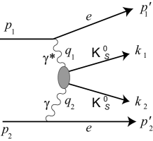
Figure 1: Feynman diagram for the process $e^{+}e^{-}\to e(e)K^{0}_{S}K^{0}_{S}$ and definition of the eight four-momenta.

A Feynman diagram for the process of interest is shown in Fig. 1, where the four-momenta of particles involved are defined. We consider the process $\gamma^{*}\gamma\to K^{0}_{S}K^{0}_{S}$ in the center-of-mass (c.m.) system of the $\gamma^{*}\gamma$. We define the $x^{*}y^{*}z^{*}$-coordinate system as shown in Fig. 2 at fixed $W$ and $Q^{2}$, where $W$ is the total energy in the $\gamma^{*}\gamma$ c.m. frame. One of the $K^{0}_{S}$ mesons is scattered at polar angle $\theta^{*}$ and azimuthal angle $\varphi^{*}$. Since the final-state particles are identical, only the region where $\theta^{*}\leq\pi/2$ and $0\leq|\varphi^{*}|\leq\pi$ is of interest. The $z^{*}$axis is defined along the incident $\gamma^{*}$ and the $x^{*}z^{*}$ plane is defined by the detected tagging $e^{\pm}$ such that $p_{{\rm tag}\,x^{*}}>0$, where $\mbox{{\boldmath$p$}}_{\rm tag}$ is the three-momentum of the tagging $e^{\pm}$.

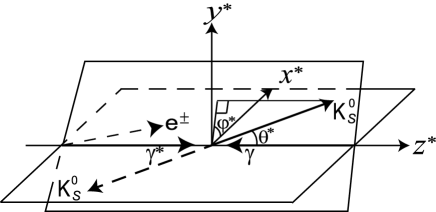
Figure 2: Definition of the $\gamma^{*}\gamma$ c.m. coordinate system for $\gamma^{*}\gamma\to K^{0}_{S}K^{0}_{S}$. The “incident” $\gamma^{*}$ has momentum along the $z^{*}$ axis with $p_{z^{*}}>0$, the tagging $e^{\pm}$ is in the $x^{*}z^{*}$ plane with $p_{{\rm tag}\,x^{*}}>0$, and the forward-going $K^{0}_{S}$ (i.e., having $p_{Kz^{*}}>0$) is produced at angles ($\theta^{*}$, $\varphi^{*}$).

The differential cross section for $\gamma^{*}\gamma\to K^{0}_{S}K^{0}_{S}$ taking place at an $e^{+}e^{-}$ collider is calculated using the helicity-amplitude formalism as follows masuda ; gss :

$$\frac{d\sigma(\gamma^{*}\gamma\to K^{0}_{S}K^{0}_{S})}{d\Omega}=\sum_{n=0}^{2}t_{n}\cos(n\varphi^{*}),$$ (1)

with

$$t_{0} = |M_{++}|^{2}+|M_{+-}|^{2}+2\epsilon_{0}|M_{0+}|^{2},$$ (2)

$$t_{1} = 2\epsilon_{1}\Re\left[(M_{+-}^{*}-M_{++}^{*})M_{0+}\right],$$ (3)

$$t_{2} = -2\epsilon_{0}\Re(M_{+-}^{*}M_{++}),$$ (4)

where $M_{++}$, $M_{0+}$, and $M_{+-}$ are separate helicity amplitudes; $+,-,0$ indicate the helicity state of the incident virtual photon along, opposite, or transverse to the quantization axis, respectively, and $\epsilon_{0}$ and $\epsilon_{1}$ are given by

$$\epsilon_{0} = \frac{1-x}{1-x+\frac{1}{2}x^{2}},$$ (5)

$$\epsilon_{1} = \frac{(2-x)\sqrt{\frac{1}{2}(1-x)}}{1-x+\frac{1}{2}x^{2}}.$$ (6)

Here, $x$ is defined as

$$x=\frac{q_{1}\cdot q_{2}}{p_{1}\cdot q_{2}},$$ (7)

where $q_{1},q_{2}$, and $p_{1}$ are the four-momenta of the virtual and real photons and an incident lepton, respectively, as defined in Fig. 1. When Eq. (1) is integrated over $\varphi^{*}$, we obtain

$$\frac{d\sigma(\gamma^{*}\gamma\to K^{0}_{S}K^{0}_{S})}{4\pi d|\cos\theta^{*}|}=|M_{++}|^{2}+|M_{+-}|^{2}+2\epsilon_{0}|M_{0+}|^{2}.$$ (8)

The total cross section is obtained by integrating Eq. (8) over $\cos\theta^{*}$, and can be written as

$$\sigma_{\rm tot}(\gamma^{*}\gamma\to K^{0}_{S}K^{0}_{S})=\sigma_{TT}+\epsilon_{0}\sigma_{LT},$$ (9)

where $\sigma_{TT}$ ($\sigma_{LT}$) corresponds to the total cross section in which both photons are transversely polarized (one photon is longitudinally polarized and the other is transversely polarized).

A $K^{0}_{S}$ pair produced in the final state of the process $e^{+}e^{-}\to e^{\pm}(e^{\mp})K^{0}_{S}K^{0}_{S}$ is a pure $C$-even state and has no contribution from single-photon production (“bremsstrahlung process”), whose effect must otherwise be considered in two-photon production of $K^{+}K^{-}$.

Schuler, Berends, and van Gulik (SBG) have calculated mesonic TFFs based on the heavy-quark approximation schuler . They found that their calculations were also applicable to light mesons with only minor modifications. The predicted $Q^{2}$ dependence of the TFFs for mesons with $J^{PC}=0^{++}$ and $2^{++}$ is summarized in Table 1, where $W$ is replaced by the equivalent mass $M$.

Table 1: Predicted $Q^{2}$ dependence of mesonic transition form factor for various helicities of the two colliding photons schuler . Each term has a common factor of $(1+Q^{2}/M^{2})^{-2}$.

$J^{PC}$	$Q^{2}$ dependence $\left[\div\left(1+\frac{Q^{2}}{M^{2}}\right)^{2}\right]$
	helicity-0	helicity-1	helicity-2
$0^{++}$	$\left(1+\frac{Q^{2}}{3M^{2}}\right)$	–	–
$2^{++}$	$\frac{Q^{2}}{\sqrt{6}M^{2}}$	$\frac{\sqrt{Q^{2}}}{\sqrt{2}M}$	1

In this paper, we report a measurement of $\gamma^{*}\gamma\to K^{0}_{S}K^{0}_{S}$, extracting for the first time the $Q^{2}$ dependence of the production cross section in the charmonium mass region (specifically for the $\chi_{c0}$ and $\chi_{c2}$ mesons), near the $K^{0}_{S}K^{0}_{S}$ mass threshold, and also the separate helicity-0, -1, and -2 TFF of the $f_{2}^{\prime}(1525)$ meson up to $Q^{2}=30~{}{\rm GeV}^{2}$. These measurements complement our earlier measurements for the corresponding no-tag process $\gamma\gamma\to K^{0}_{S}K^{0}_{S}$ over the range $1.05~{}{\rm GeV}\leq W\leq 4.0~{}{\rm GeV}$ ksks .

II Experimental apparatus and Data Sample

We use a 759 fb^-1 data sample recorded with the Belle detector belle ; belleptep at the KEKB asymmetric-energy $e^{+}e^{-}$ collider kekb ; kekb2 ; this data sample is identical to that used for the previous $\gamma^{*}\gamma\to\pi^{0}\pi^{0}$ measurement masuda .

II.1 Belle detector

A comprehensive description of the Belle detector is given elsewhere belle ; belleptep . In the following, we describe only the detector components essential for this measurement. Charged tracks are reconstructed from the drift-time information in a central drift chamber (CDC) located in a uniform 1.5 T solenoidal magnetic field. The $z$ axis of the detector and the solenoid is opposite the positron beam. The CDC measures the longitudinal and transverse momentum components, i.e., along the $z$ axis and in the $r\varphi$ plane perpendicular to the beam, respectively. The trajectory coordinates near the collision point are measured by a silicon vertex detector. A barrel-like arrangement of time-of-flight (TOF) counters is used to supplement the CDC trigger for charged particles and to measure their time of flight. Charged-particle identification (ID) is achieved by including information from the CDC, the TOF, and an array of aerogel threshold Cherenkov counters. Photon detection and energy measurements are performed with a CsI(Tl) electromagnetic calorimeter (ECL) by clustering the ECL energy deposits not matched to extrapolated CDC charged track trajectories. Electron identification is based on $E/p$, the ratio of the ECL calorimeter energy to the CDC track momentum.

II.2 Triggers

The triggers that are important for this analysis are the ECL-based ecltrig HiE (High-energy threshold) trigger and the Clst4 (four-energy-cluster) energy triggers. The HiE trigger requires that the sum of the energies measured by the ECL in an event exceed 1.15 GeV, but that the event topology not be similar to Bhabha scattering (“Bhabha veto”); the latter requirement is enforced by the absence of the CsiBB trigger, which is designed to identify back-to-back Bhabha events ecltrig . The Clst4 trigger requires at least four separated energy clusters in the ECL with each cluster energy above 0.11 GeV; this trigger is not vetoed by the CsiBB. Five clusters are expected in total in the signal events of interest if all the final-state particles are detected within the fiducial volume of the ECL trigger ($18.5^{\circ}<\theta<128.6^{\circ}$).

Belle employs many distinct track triggers that require anywhere from two to four CDC tracks, in conjunction with pre-specified TOF and/or ECL information. Among these track triggers, the Bhabha veto is applied to the two-track triggers only.

The candidate signal topology nominally has five tracks and one high-energy cluster from the electron. Over the entire kinematic range of interest, the trigger efficiency is in general quite high, owing to the trigger requirements demanding two or three CDC tracks with TOF and ECL hits, with the exception of the lowest $Q^{2}$ region probed in this analysis, where the particles tend to scatter into very small polar-angle regions. The typical trigger efficiency is 95%, with slightly lower efficiency (around 90%) for events having both $W\leq 1.5~{}{\rm GeV}$ and $Q^{2}\leq 5~{}{\rm GeV}^{2}$.

II.3 Signal Monte Carlo

We use the signal Monte Carlo (MC) generator, TREPSBSS, which has been developed to calculate the efficiency for single-tag two-photon events, $e^{+}e^{-}\to e(e)X$, as well as the two-photon luminosity function for $\gamma^{*}\gamma$ collisions at an $e^{+}e^{-}$ collider , following our previous $\pi^{0}\pi^{0}$ study masuda ; treps .

We choose fifteen different $W$ points between 1.0 GeV and 3.556 GeV, including two $\chi_{cJ}$ ($J$ =0, 2) mass points, for the calculation of the luminosity function and event generation. The luminosity function is defined as the conversion factor from the $e^{+}e^{-}$-based differential cross section, $d^{2}\sigma_{ee}/dWdQ^{2}$, to the $\gamma^{*}\gamma$-based cross section, $\sigma(W,Q^{2})$ masuda . The scattering angle of the $K^{0}_{S}$ is uniformly distributed in the $\gamma^{*}\gamma$ c.m. system in the MC sample. To properly weight our MC sample by the beam-energy distributions used for the data analysis, we generate $4\times 10^{5}$ events [$8\times 10^{4}$ events] for the beam energy point of $\Upsilon(4S)$ [$\Upsilon(5S)$].

We use a GEANT3-based detector simulation geant to study the propagation of the generated particles and their daughters through the detector. The $K^{0}_{S}$ pairs decay generically in the detector simulator. The same code used for analysis of true data is used for reconstruction and selection of the MC simulated events.

III Event Selection

Event selection parallels that of our previous $\pi^{0}\pi^{0}$ analysis masuda . Here, we also present comparisons between data and simulation for our selected $K^{0}_{S}K^{0}_{S}$ samples.

III.1 Selection criteria

A candidate $e^{+}e^{-}\to e(e)K^{0}_{S}K^{0}_{S}$ signal event with $K^{0}_{S}$ decaying to $\pi^{+}\pi^{-}$ contains an energetic tagging electron and four charged pions. The kinematic variables are calculated in the laboratory system unless otherwise noted; those in the $e^{+}e^{-}$ or $\gamma^{*}\gamma$ c.m. frame are identified with an asterisk in this section.

We require exactly five tracks satisfying $p_{t}>0.1~{}{\rm GeV}/c$, $dr<5$ cm, and $|dz|<5$ cm. Among these, at least two tracks must satisfy $p_{t}>0.4~{}{\rm GeV}/c$, $-0.8660<\cos\theta<0.9563$, and $dr<1$ cm. Here, $p_{t}$ is the transverse momentum in the laboratory frame, $\theta$ is the polar angle of the momentum, and ($dr$, $dz$) are the cylindrical coordinates of the point of closest approach of the track to the nominal $e^{+}e^{-}$ primary interaction point; all four variables are measured with respect to the $z$ axis.

One of the tracks having $p_{t}>0.4$ GeV/$c$ and $p>1.0$ GeV/$c$ must also be electron- (or positron-) like. This is ensured by requiring that the ratio of the candidate calorimeter cluster energy, using the cluster-energy correction outlined previously masuda , relative to the absolute momentum satisfy $E/p>0.8$.

We search for exactly two $K^{0}_{S}$ candidates, each of which is reconstructed from a unique charged-pion pair. Each pion satisfies the $K/\pi$ particle ID separation criterion ${\cal L}_{K}/({\cal L}_{K}+{\cal L}_{\pi})<0.8$, which is applied for the likelihood probability ratio for the hadron identification hypotheses obtained by combining information from the particle-ID detectors. The invariant mass of the $K^{0}_{S}$ candidates at the reconstructed decay vertex must be within $\pm 20$ MeV/$c^{2}$ of the nominal $K^{0}_{S}$ mass, 0.4976 GeV/$c^{2}$ pdg2016 .

After the two $K^{0}_{S}$ candidates are found, we refine the event selection by additionally requiring that the average of, and difference between, the masses of the two $K^{0}_{S}$’s be within $\pm 5$ MeV/$c^{2}$ from the nominal $K^{0}_{S}$ mass, and smaller than 10 MeV/$c^{2}$, respectively ksks . Each $K^{0}_{S}$ decay vertex must lie within the cylindrical volume defined by $0.3\,{\rm cm}<r_{VK}<8\,{\rm cm}$ and $-5\,{\rm cm}<z_{VK}<+7\,{\rm cm}$, where ($r_{VK}$, $z_{VK}$) is the decay-vertex position of the $K^{0}_{S}$.

We do not require the characteristic relation between the $z$ component of the observed total momenta and the charge of the tagging lepton that was used in the previous $\pi^{0}\pi^{0}$ analysis masuda , as this results in no effective additional background reduction; the background from $e^{+}e^{-}$ annihilation is already very small, given our distinctive event topology.

We apply an acoplanarity cut between the c.m. momenta of the electron and the two-$K^{0}_{S}$ system, namely, that their opening angle projected onto the $r\varphi$ plane must exceed $\pi-0.1$ radians.

Finally, we apply kinematic selection using the $E_{\rm ratio}$ and $p_{t}$-balance variables just as was done for the $\pi^{0}\pi^{0}$ selection masuda . Those definitions of $E_{\rm ratio}$ and $p_{t}$ balance are reproduced here for completeness. The energy ratio is

$$E_{\rm ratio}=\frac{E^{*{\rm measured}}_{K^{0}_{S}K^{0}_{S}}}{E^{*{\rm expected}}_{K^{0}_{S}K^{0}_{S}}},$$ (10)

where $E^{*{\rm measured}}_{K^{0}_{S}K^{0}_{S}}$ ($E^{*{\rm expected}}_{K^{0}_{S}K^{0}_{S}}$) is the $e^{+}e^{-}$ c.m. energy of the $K^{0}_{S}K^{0}_{S}$ system measured directly (as expected by kinematics, assuming no radiation). The $p_{t}$-balance $|\Sigma\mbox{{\boldmath$p$}}_{t}^{*}|$ is defined by

$$|\Sigma\mbox{{\boldmath$p$}}_{t}^{*}|=|\mbox{{\boldmath$p$}}^{*}_{t,e}+\mbox{{\boldmath$p$}}^{*}_{t,K1}+\mbox{{\boldmath$p$}}^{*}_{t,K2}|.$$ (11)

We require that the quadratic combination of the two variables ($E_{\rm ratio}$ and $|\Sigma\mbox{{\boldmath$p$}}_{t}^{*}|$) satisfy

$$\sqrt{\left(\frac{E_{\rm ratio}-1}{0.04}\right)^{2}+\left(\frac{|\Sigma\mbox{{\boldmath$p$}}_{t}^{*}|}{0.1~{}{\rm GeV}/c}\right)^{2}}\leq 1.$$ (12)

We assign four kinematic variables — $Q^{2}$, $W$, $|\cos\theta^{*}|$, and $|\varphi^{*}|$ — to each candidate event, similar to the $\pi^{0}\pi^{0}$ analysis masuda .

III.2 Distributions of the signal candidates and comparison with the signal-MC events

In this subsection, we present various distributions of the selected signal candidates. The backgrounds are expected to be quite low in the experimental data. Some of the data distributions are compared with those of the signal-MC samples, where a uniform angular distribution and a representative $Q^{2}$ dependence masuda are assumed.

The experimental $W$ distribution for events passing our selection criteria is shown in Fig. 3 for $W\leq$ 3.8 GeV. A structure corresponding to the tensor $f^{\prime}_{2}(1525)$ resonance is clearly visible. We also note an apparent enhancement near the $K^{0}_{S}K^{0}_{S}$ mass threshold, that may be associated with the $f_{0}(980)$ and/or the $a_{0}(980)$ mesons. We find 124 (14) events in the region $W<3.0~{}{\rm GeV}$ and $3~{}{\rm GeV}^{2}<Q^{2}<30~{}{\rm GeV}^{2}$ ($3.0~{}{\rm GeV}<W<3.8~{}$GeV and $2~{}{\rm GeV}^{2}<Q^{2}<30~{}{\rm GeV}^{2}$).

We now focus on events having $W\leq 2.6$ GeV and the two $\chi_{cJ}$($J=0,2$) mass regions, where we detect the signal process with a high efficiency and a good signal-to-noise ratio. For the same reason, we also constrain the $Q^{2}$ region to 3 GeV${}^{2}\leq Q^{2}\leq 30$ GeV² (2 GeV${}^{2}\leq Q^{2}\leq 30$ GeV²) for $W\leq 2.6$ GeV (the $\chi_{cJ}$ mesons).

For comparison, the corresponding distributions from the signal MC in this kinematic regime are shown in Figs. 4 – 6. In our analysis, we sometimes differentiate electron-tag (e-tag) from positron-tag (p-tag) to facilitate studies of systematics. We find that the p-tag has a much higher efficiency than that of the e-tag in the lowest $Q^{2}$ region, where the cross section is large (Fig. 4).

Figure 5 compares the measured distributions of the reconstructed $\pi^{+}\pi^{-}$ invariant mass at each $K^{0}_{S}$-candidate decay vertex with MC in three different $W$ ranges, as indicated above each panel pair. All the selection criteria, except those related to the reconstructed $K^{0}_{S}$ invariant masses ($M_{Ki}$), have been applied to the sample. Non-$K^{0}_{S}$ background is seen to be small.

Figure 6 shows the cosine of the polar angle of the tagging electron, that of the neutral kaon, and the energy of the neutral kaon in the laboratory frame for the sample at $W<3.0$ GeV and 3 GeV${}^{2}\leq Q^{2}\leq 30$ GeV². They all show satisfactory agreement, given the approximate $Q^{2}$ and isotropic angular dependence in the signal-MC sample.

Two-dimensional plots for $p_{t}$ balance ($|\Sigma\mbox{{\boldmath$p$}}_{t}^{*}|$) vs. $E_{\rm ratio}$ are shown in Fig. 7. We find that there are backgrounds with a slightly smaller $E_{\rm ratio}$ and slightly larger $p_{t}$ imbalance for the data at $W<1.3$ GeV. These are considered to arise from the non-exclusive backgrounds $\gamma^{*}\gamma\to K^{0}_{S}K^{0}_{S}X$, where $X$ is a $\pi^{0}$ or some combination of otherwise undetected particles. We discuss and subtract the background contamination of this component in the next sections. Such a large background contamination is not observed for $W>1.3$ GeV.

Figure 3: The experimental $W$ distributions of the signal candidates at 2 GeV² (3 GeV²) $<Q^{2}<30$ GeV² as indicated by the asterisks (dashed histogram). Backgrounds have not been subtracted.

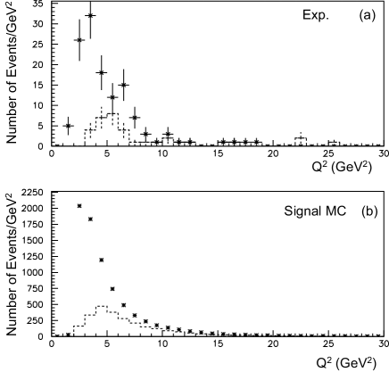
Figure 4: (a) The $Q^{2}$ distributions for the data samples at $W\leq 4.0$ GeV. The asterisks and the dashed histogram are for the p-tag and e-tag samples, respectively. (b) The corresponding distributions from the signal MC events. Statistics of the MC figures are arbitrary, but the scale is common for the e- and p-tags in each panel, so that their ratio can be compared between MC and data.

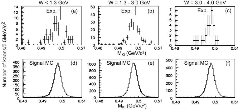
Figure 5: (a,b,c) Reconstructed $\pi^{+}\pi^{-}$ invariant mass, as measured at each determined decay vertex for the data, in three different $W$ ranges, as indicated above each panel. (d,e,f) The corresponding distributions from the signal MC.

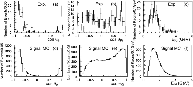
Figure 6: The distributions for experimental signal candidates (top row) and signal MC (bottom row) for (a,d) the cosine of the laboratory polar angle of the tagging electron, (b,e) the cosine of the laboratory polar angle of the two $K^{0}_{S}$ candidates (two entries per event), and (c,f) the laboratory energy of the two $K^{0}_{S}$ candidates (two entries per event).

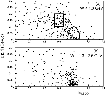
Figure 7: Distribution of $p_{t}$ balance vs. $E_{\rm ratio}$ for the experimental samples to which the selection criteria other than those related to the illustrated variables have been applied. The $W$ region for the samples is shown in each panel. The half-ellipse and the rectangle in (a) show the signal and control regions, respectively.

IV Background estimation

IV.1 Non-$K^{0}_{S}$ background processes

Backgrounds may arise from events in which there are either zero or only one true $K^{0}_{S}$. The latter may include contributions from $K^{0}_{S}K^{\pm}\pi^{\mp}$. The backgrounds from these processes are expected to be largely eliminated by requirements on the invariant mass and flight length for each of the neutral kaon candidates.

If such a background component were present in the data, we would expect an event concentration at $r_{VKi}<0.2$ cm, based on studies of non-resonant $\pi^{+}\pi^{-}\pi^{+}\pi^{-}$ and $K^{0}_{S}K^{\pm}\pi^{\mp}$ processes, using both the MC and background-enriched data samples. In Figs. 8(a) and 8(b), we show the distribution of $r_{VKi}$ for the case $r_{VKj}>0.3$ cm ($j\neq i$) for experimental events where the criteria other than $r_{VKi}$ have been applied, separately for the two $W$ regions. These are consistent with the signal-MC distributions shown in Figs. 8(c) and 8(d). According to this study, the background from this source is estimated to be less than one event in the entire data sample, so we neglect its contribution.

IV.2 Non-exclusive background processes

The non-exclusive background processes, $e^{+}e^{-}\to e(e)K^{0}_{S}K^{0}_{S}X$, where $X$ denotes one or multiple hadrons, are in general subdivided into two-photon ($C$-even) and virtual pseudo-Compton (bremsstrahlung, $C$-odd) processes, although these may interfere with each other if the same $X$ is allowed for both processes. The majority of such background events populate the small-$E_{\rm ratio}$ and large-$p_{t}$ imbalance region, e.g., $(E_{\rm ratio}<0.8)~{}\cap~{}(|\Sigma\mbox{{\boldmath$p$}}_{t}^{*}|>0.1$ GeV/$c$). This feature is distinct from the aforementioned background processes that can populate the region near $E_{\rm ratio}=1$ and peak near $|\Sigma\mbox{{\boldmath$p$}}_{t}^{*}|=0$.

To further assess background contributions, we consider the correlation between these two variables in the experimental sample, as illustrated in Fig. 7. We estimate the relative ratio of the number of non-exclusive background events to the signal yield by counting the number of events in the control region outside the signal region, that is, $(0.87<E_{\rm ratio}<0.93)\cap(0.1~{}{\rm GeV}/c<|\Sigma\mbox{{\boldmath$p$}}_{t}^{*}|<0.2~{}{\rm GeV}/c)$ where the background component would be relatively large, as well as in the selected signal region [Fig. 7(a)]. The $W$ dependence of the number of events thus obtained in the signal and control regions is shown in Figs. 9(a) and 9(b), respectively. The peak in the 1.0 – 1.2 GeV region for the control samples implies that the signal samples include a significant background in the same $W$ region.

We generate background $K^{0}_{S}K^{0}_{S}\pi^{0}$ final-state MC events, which distribute uniformly in phase space, to estimate the background contamination in the signal region. The estimation using this process, which corresponds to the minimum particle multiplicity of $X$, leads to a conservative (i.e., on the larger side) estimate for the background fraction, since such backgrounds tend to distribute themselves close to the signal region.

The expected ratio of the background magnitude in the signal region to that in the control region ($f_{\rm bs}$) is 13%. We also estimate the ratio of the signal events falling in the control region to that in the signal region ($f_{\rm sc}$) to be 5.6%. We determine the expected background-component ratio in the sample in the signal region, $f_{\rm bs}n_{\rm b}/N_{\rm s}$, by solving simultaneous linear equations, $N_{\rm s}=n_{\rm s}+f_{\rm bs}n_{\rm b}$ and $N_{\rm c}=f_{\rm sc}n_{\rm s}+n_{\rm b}$, where $N_{\rm s}$ $(N_{\rm c})$ is the number of observed events in the signal (control) region, and $n_{\rm s}$ $(n_{\rm b})$ is the number of the signal (background) events in the signal (control) region. The background component thus obtained is 14% of the entire candidate event sample at $W<1.3$ GeV. Above 1.3 GeV, the background is less than 1% and is negligibly small.

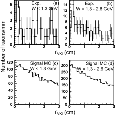
Figure 8: (a,b) Experimental distribution of $r_{VKi}$ ($r$ coordinate of the $\pi^{+}\pi^{-}$ vertex point for a $K^{0}_{S}$ candidate) for an event in which the other kaon-vertex coordinate satisfies the selection criterion $r_{VKj}>0.3$ cm. The $W$ region for each sample is shown in each panel. The vertical arrows indicate the selection criterion. (c,d) The corresponding distributions from the signal-MC samples. Statistics of the MC figures are arbitrary.

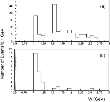
Figure 9: The $W$ distribution of experimental-data events in (a) the signal region and (b) the control region.

V Derivation of the cross section

Similarly to the derivation of the $\pi^{0}\pi^{0}$ cross section masuda , we first define and evaluate the $e^{+}e^{-}$-based cross section separately for the p-tag and e-tag samples. After confirming the consistency between the p- and e-tag measurements to ensure validity of the efficiency corrections, we combine their yields and efficiencies. We then convert the $e^{+}e^{-}$-incident-based differential cross section to that based on $\gamma^{*}\gamma$-incident by dividing by the single-tag two-photon luminosity function $d^{2}L_{\gamma^{*}\gamma}/dWdQ^{2}$, which is a function of $W$ and $Q^{2}$. We use the relation

$$\sigma_{\rm tot}(\gamma^{*}\gamma\to K^{0}_{S}K^{0}_{S})=\frac{1}{2\frac{d^{2}L_{\gamma^{*}\gamma}}{dWdQ^{2}}}\times$$

$$\frac{Y(W,Q^{2})}{(1+\delta)\varepsilon(W,Q^{2})\Delta W\Delta Q^{2}\!\int\!{\cal L}dt{\cal B}^{2}},$$ (13)

where $Y$ is the yield and $\varepsilon$ is the efficiency obtained by the signal MC. Here, the factor $\delta$ corresponds to the radiative correction, $\int{\cal L}dt$ is the integrated luminosity of 759 fb^-1, and ${\cal B}^{2}=0.4789$ is the square of the decay branching fraction ${\cal B}(K^{0}_{S}\to\pi^{+}\pi^{-})$. The measurement ranges of $W$ and $Q^{2}$, and the corresponding bin widths $\Delta W$ and $\Delta Q^{2}$, are summarized in Table 2. Our measurement extends down to the mass threshold $W=2m_{K^{0}_{S}}$, where $m_{K^{0}_{S}}$ is the mass of $K^{0}_{S}$ pdg2016 . For bins for $W>1.2$ GeV, the cross section is first calculated with $\Delta W=0.05$ GeV, and then its values in two or four adjacent bins are combined, with the point plotted at the arithmetic mean of the entries in that combined bin.

Table 2: The measurement range and bin widths defining the bins in the two-dimensional $(W,Q^{2})$ space.

Variable	Measurement	Bin width	Unit	Number
	range			of bins
$W$	0.995($2m_{K^{0}_{S}}$) – 1.05	0.055	GeV	1
	1.05 – 1.2	0.05		3
	1.2 – 1.6	0.1		4
	1.6 – 2.6	0.2		5
$Q^{2}$	3.0 – 7.0	2.0	GeV2	2
	7.0 – 10.0	3.0		1
	10.0 – 15.0	5.0		1
	15.0 – 30.0	15.0		1

V.1 Efficiency plots and consistency check for the p-tag and e-tag measurements

Figure 10 shows the aggregate efficiencies, as a function of $W$ for the selected $Q^{2}$ bins of the p- or e-tag samples, including all event selection and trigger effects. These efficiencies are obtained from the signal-MC events, which are generated assuming an isotropic $K^{0}_{S}$ angular distribution in the $\gamma^{*}\gamma$ c.m. frame.

Our accelerator and detector systems are asymmetric between the positron and electron incident directions and energies, and separate measurements of the p-tag and e-tag samples provide a good internal consistency check for various systematic effects of the trigger, detector acceptance, and selection conditions. Figure 11 compares the $e^{+}e^{-}$-based cross section measured separately for the p- and e-tags. They are expected to show the same cross section according to the $C$ symmetry if there is no systematic bias. In this figure, the estimated non-exclusive backgrounds are subtracted, fixing the ratio of the values from the p- and e-tag measurements.

The results from the two tag conditions are consistent within statistical errors. We therefore combine the p- and e-tag sample results using their summed yields and averaged efficiencies.

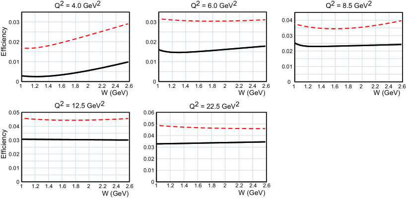
Figure 10: Efficiency (including trigger effects) as estimated from the signal-MC samples. The solid (black) and dashed (red) curves are for e-tag and p-tag events, respectively. Results are shown for five $Q^{2}$ regions, whose central values are indicated above each panel.

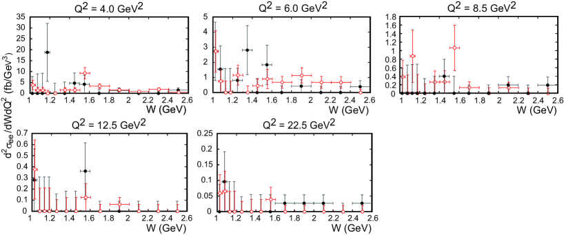
Figure 11: The efficiency-corrected and background-subtracted $W$ dependence of the $e^{+}e^{-}$-based cross section in each $Q^{2}$ bin. The black closed (red open) circles with error bars are for the e-tag (p-tag) measurements. The red p-tag points have been shifted slightly to the right for enhanced visibility.

V.2 Derivation of angle-integrated $\gamma^{*}\gamma\to K^{0}_{S}K^{0}_{S}$ cross section

We apply a radiative correction of 2% to the total cross section. This value is the same as that evaluated in the analogous case of single pion production pi0tff . This correction depends only slightly on $W$ and $Q^{2}$, and is treated as a constant. The radiative effect in the event topology is taken into account in the signal-MC event generation and is reflected in the efficiency calculation.

To account for the non-linear dependence on $Q^{2}$, we define the nominal $Q^{2}$ for each finite-width bin $\overline{Q}^{2}$, using the formula

$$\frac{d\sigma_{ee}}{dQ^{2}}(\overline{Q}^{2})=\frac{1}{\Delta Q^{2}}\int_{\rm bin}\frac{d\sigma_{ee}}{dQ^{2}}(Q^{2})dQ^{2},$$ (14)

where $\Delta Q^{2}$ is the bin width. We assume an approximate dependence of $d\sigma/dQ^{2}\propto Q^{-7}$ for this calculation pi0tff , independent of $W$. The $\overline{Q}^{2}$ values thus obtained are listed in Table 3. We use the luminosity function at a given $\overline{Q}^{2}$ point to obtain the $\gamma^{*}\gamma$-based cross section for each $Q^{2}$ bin. We also list the central value of the $Q^{2}$ bins; these are used for convenience to represent the individual bins in tables and figures.

Table 3: The nominal $Q^{2}$ value ($\overline{Q}^{2}$) for each $Q^{2}$ bin.

$Q^{2}$ bin (GeV2)	Bin center (GeV2)	$\overline{Q}^{2}$ (GeV2)
2 – 3	2.5	2.42
3 – 5	4.0	3.81
5 – 7	6.0	5.87
7 – 10	8.5	8.30
10 – 15	12.5	12.1
15 – 30	22.5	20.6

The $Q^{2}$ value measured for each event can differ from the true $Q^{2}$ for two primary reasons: the finite resolution in our $Q^{2}$ determination and/or the reduction of the incident electron energy due to initial-state radiation (ISR). However, the relative $Q^{2}$ resolution in the measurement, typically 0.7%, which is estimated using the signal-MC events, is much smaller than the typical bin sizes and therefore has a negligible effect. The ISR effect is also negligibly small in this analysis owing to the tight $E_{\rm ratio}$ selection criterion, which rejects events with high-energy radiation. Thus, we do not apply the $Q^{2}$-unfolding procedure in this analysis, which was applied in the previous analysis where the corresponding selection condition was less restrictive masuda .

The $e^{+}e^{-}$-based differential cross sections thus measured are converted to $\gamma^{*}\gamma$-based cross sections, corresponding to $\sigma_{\rm tot}(\gamma^{*}\gamma\to K^{0}_{S}K^{0}_{S})=\sigma_{\rm TT}~{}+~{}\epsilon_{0}\sigma_{\rm LT}$, using the luminosity function as described above. Figure 12 shows the total cross sections (integrated over angle) for the single-tag two-photon production of $K^{0}_{S}K^{0}_{S}$, as a function of $W$ in five $Q^{2}$ bins.

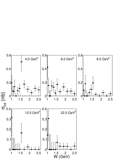
Figure 12: Total cross sections (integrated over angle) for $\gamma^{*}\gamma\to K^{0}_{S}K^{0}_{S}$ in the five $Q^{2}$ bins indicated in each panel.

V.3 Helicity components and angular dependence

We now estimate $\epsilon_{0}$ and $\epsilon_{1}$, the factors that appear in Eqs. (2) – (4), in each $(W,Q^{2})$ bin. We use the mean value of $\epsilon_{0}$ ($\epsilon_{1}$) as calculated by Eq. (5) [Eq. (6)] for the selected events from the signal-MC samples, as they depend only very weakly on $Q^{2}$ and $W$. The numerical values in the kinematic range $W<1.8\,{\rm GeV}$ are summarized in Table 4, where we neglect the $W$ dependence because it is small (within $\pm 2\%$); here, we apply the partial-wave analysis of Sec. VI.

For analysis of the three helicity components 0, 1, and 2 described in Sec. VI.3, we use a normalized angular-differentiated cross section (integrated over $Q^{2}$) $(d^{2}\sigma/d|\cos\theta^{*}|d|\varphi^{*}|)/\sigma$, which is derived as follows. We assume that the angular dependence of $d^{2}\sigma/d|\cos\theta^{*}|d|\varphi^{*}|$ follows $N_{\rm EXP}(|\cos\theta^{*}|,|\varphi^{*}|)/N_{\rm MC}(|\cos\theta^{*}|,|\varphi^{*}|)$ in each $W$ bin integrated in the $Q^{2}=$ 3 – 30 GeV² region and take this to be the angular dependence at $Q^{2}=\langle Q^{2}\rangle=6.5$ GeV², where $\langle Q^{2}\rangle$ is the mean value of $Q^{2}$ for all the selected experimental events. For this purpose, we use four $W$ bins starting at the mass threshold: 0.995  – 1.2 GeV, 1.2 – 1.4 GeV, 1.4 – 1.6 GeV, and 1.6 – 1.8 GeV. The angular bin sizes are $\Delta|\cos\theta^{*}|=0.2$ and $\Delta|\varphi^{*}|=30^{\circ}$. We use the normalization $\int_{0}^{1}d|\cos\theta^{*}|\int_{0}^{\pi}d|\varphi^{*}|[(d^{2}\sigma/d|\cos\theta^{*}|d|\varphi^{*}|)/\sigma]=1$.

Table 4: The values of the $\epsilon_{0}$ and $\epsilon_{1}$ parameters, as a function of $Q^{2}$, at $W<1.8$ GeV.

$Q^{2}$ bin (GeV2)	$\epsilon_{0}$	$\epsilon_{1}$
3 – 5	0.92	1.33
5 – 7	0.91	1.32
7 – 10	0.89	1.30
10 – 15	0.87	1.28
15 – 30	0.82	1.23

V.4 Derivation of the partial decay width of the $\chi_{cJ}$ mesons

We find a clear excess of events in the mass region of the $\chi_{cJ}$ ($J=0,2$) mesons as shown in Fig. 3. We define signal regions to be 3.365 – 3.465 GeV/$c^{2}$ and 3.505 – 3.605 GeV/$c^{2}$ for the $\chi_{c0}$ and $\chi_{c2}$ mesons, respectively, and note that the process $\chi_{c1}\to K^{0}_{S}K^{0}_{S}$ is prohibited by parity conservation. We measure over the range 2 GeV${}^{2}\leq Q^{2}\leq 30$ GeV², and expect a much better efficiency in the $\chi_{cJ}$ mass region at small $Q^{2}$ than in the lower-$W$ region.

The charmonium yields in the $Q^{2}$ range are 7 and 3 for the $\chi_{c0}$ and $\chi_{c2}$ mesons, respectively; we assume, given the evident absence of background, that they are pure contributions from charmonia. Based on studies of no-tag $K^{0}_{S}K^{0}_{S}$ ksks and single-tag $\pi^{0}\pi^{0}$ masuda measurements, we similarly estimate less than one background event for the total of the two charmonium regions.

We first determine the $e^{+}e^{-}$-based cross section in the two $\chi_{cJ}$ mass regions. This is then translated to the product of the two-photon decay width and the branching fraction into the $K^{0}_{S}K^{0}_{S}$ final state using the relation

$$\frac{d\sigma_{ee}}{dQ^{2}} = 4\pi^{2}\left(1+\frac{Q^{2}}{M_{R}^{2}}\right)\frac{(2J+1)}{M_{R}^{2}}\frac{2d^{2}L_{\gamma^{*}\gamma}}{dWdQ^{2}}$$ (15)

$$\times\,\Gamma_{\gamma^{*}\gamma}(Q^{2}){\cal B}(K^{0}_{S}K^{0}_{S}),$$

which is valid for a narrow resonance after integrating over $W$, where $M_{R}$ is the resonance mass. It is not possible to present the $\chi_{cJ}$ production rate as a function of $\sigma_{\gamma^{*}\gamma}(W,Q^{2})$ because we know that each of the $\chi_{cJ}$ mesons has a narrow but finite width that is comparable to the resolution of our measurement. Instead, we present the two-photon decay width $\Gamma_{\gamma^{*}\gamma}(Q^{2})$ with the above formula, which we define similarly to the TFF in Eq. (19) with respect to the functional dependence on $Q^{2}$.

Note that the three independent helicity amplitudes are effectively added in this definition, assuming unpolarized $e^{+}e^{-}$ collisions for the $\chi_{c2}$ meson, and this formula can be considered as the definition of $\Gamma_{\gamma^{*}\gamma}(Q^{2})$ at $Q^{2}>0$; we adopt it as such in what follows.

Figure 13 shows the $Q^{2}$ dependence of $\Gamma_{\gamma^{*}\gamma}/\Gamma_{\gamma\gamma}$ for the $\chi_{c0}$ and $\chi_{c2}$ mesons, where $\Gamma_{\gamma\gamma}$ is the value for the real two-photon decay, which is extracted from the $\Gamma_{\gamma\gamma}{\cal B}(K^{0}_{S}K^{0}_{S})$ world-average values of ($7.3~{}\pm~{}0.6$) eV and ($0.291~{}\pm~{}0.025$) eV for the $\chi_{c0}$ and $\chi_{c2}$ mesons, respectively pdg2016 . This is the first measurement of $\chi_{cJ}$ charmonium production in high-$Q^{2}$ single-tag two-photon collisions.

These measurements are compared to the SBG schuler predictions evaluated at the $\chi_{cJ}$ mass and also the expectation using a vector-dominance model (VDM) sakurai with the $\rho$ mass in the factor $(1+Q^{2}/m_{\rho}^{2})^{-2}$. As can be clearly seen, the low statistics notwithstanding, we obtain reasonable agreement with SBG prediction at the charmonium-mass scale.

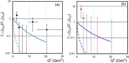
Figure 13: $Q^{2}$ dependence of $\Gamma_{\gamma^{*}\gamma}$ for the (a) $\chi_{c0}$ and (b) $\chi_{c2}$ mesons normalized to $\Gamma_{\gamma\gamma}$ (at $Q^{2}=0$) pdg2016 . The data point without a dot is based on a zero-event observation, and the upper edge of its error bar corresponds to the value for one event. The overall uncertainties due to the normalization errors of the $\Gamma_{\gamma\gamma}{\cal B}(K^{0}_{S}K^{0}_{S})$ are not shown. The solid and dashed curves, respectively, show the SBG schuler prediction and also one motivated by VDM, assuming $\rho$ dominance.

V.5 Systematic uncertainties

We estimate systematic uncertainties in the measurement of the differential cross section as summarized in Table 5.

V.5.1 Uncertainties in the efficiency evaluation

The detection efficiency is evaluated using signal-MC events. However, our simulation has some known mismatches with data that translates into uncertainties in the efficiency evaluation.

Charged particle tracking has a 2% uncertainty for five tracks, which is estimated from a study of the decays $D^{*\pm}\to D^{0}\pi^{\pm},D^{0}\to K^{0}_{S}(\to\pi^{+}\pi^{-})\pi^{+}\pi^{-}$ (0.35% per track) including an uncertainty in the radiation by an electron within the CDC volume (about 1%, added in quadrature).

The electron identification efficiency in this measurement is very high, around 98%, and a 1% systematic uncertainty is assigned to it. Detection of the $\pi^{+}\pi^{-}$ pairs for reconstructing two $K^{0}_{S}$ mesons has a 2% uncertainty due to the requirement to identify four charged pions, and another 3% for $K^{0}_{S}$ reconstruction and selection dominated by a possible difference in the mass resolution for the reconstructed $K^{0}_{S}$ between the experiment and the signal MC.

Our kinematic condition based on the $E_{\rm ratio}$ and $p_{t}$ balance has an accompanying uncertainty of 4%. In addition, imperfections in modeling detector edge locations and other geometrical-description effects result in an uncertainty of 1%.

The uncertainty of the trigger efficiency is estimated using different types of subtrigger components, with special attention given to events satisfying multiple trigger conditions. We select four kinds of primary subtriggers whose efficiencies are well-studied. The first two are distinct possible two track triggers: one requires total energy activity in the ECL exceeding 0.5 GeV, and the other requires an ECL cluster as well as two TOF hits. The other two trigger lines are the neutral triggers, namely HiE and Clst4.

More than half of the signal candidates are triggered by two or more distinct triggers. We estimate the uncertainty on the trigger inefficiency as a fractional difference of the efficiencies between the cases for which all the subtrigger components are ORed and the case where at least one of the selected four triggers is fired. This uncertainty is estimated to be 3% for $W<2.6~{}{\rm GeV}$ and 1% for the $\chi_{cJ}$ charmonium-mass region.

Backgrounds overlapping with the signal events may reduce the efficiency; this effect is accounted for in MC simulations by embedding hits from a non-triggered event (“random” or “unbiased” triggers) in each signal-MC event. We evaluate this effect separately for each different beam-condition state and run period. The corresponding effect on the efficiency is estimated to be 2%.

We take into account an uncertainty on the efficiency-correction factor arising from the angular dependence of the differential cross section. This correction arises when both the selection efficiency and differential cross sections have angular nonuniformities. As we do not measure the angular dependence of the differential cross section for different kinematic regions owing to limited statistics, we assume several typical angular dependences of the differential cross section based on the spherical-harmonic functions of $J\leq 2$: proportional to $\cos\theta^{*}$, $\cos^{2}\theta^{*}$, $(3\cos^{2}\theta^{*}-1)^{2}$, $\sin^{4}\theta^{*}$, $(1+0.5\cos\varphi^{*})$, and $(1+0.5\cos 2\varphi^{*})$.

We examine the efficiency differences for these angular-dependence shapes from that of the isotropic-efficiency case using simulated events, and assign its typical variation size, taking a quadratic sum of the $\cos\theta^{*}$ and $\varphi^{*}$ contributions, to the systematic uncertainty from this source. The $W$-dependent estimated error magnitude is 6% – 22%: this dependence originates purely from the difference in the degree of nonuniformity in the efficiency.

V.5.2 Uncertainties from other sources

We assign 7%, half of the magnitude of the subtraction itself, as the uncertainty in the background subtractions arising from $K^{0}_{S}K^{0}_{S}X$ non-exclusive processes for $W<1.3~{}$GeV. We assign 3% as the uncertainty for the other $W$ regions. Other background sources are negligibly small.

The omission of the $Q^{2}$-unfolding procedure introduces an uncertainty of 1%. The radiative correction has an uncertainty of 3%. The evaluation of the luminosity function gives an uncertainty of 4%, including a model uncertainty for the form factor of the untagged side (2%) masuda . The integrated luminosity measurement has an uncertainty of 1.4%.

The systematic uncertainties are added in quadrature unless noted above. The total systematic uncertainty is between 13% and 24%, depending on the $W$ bins.

Table 5: Sources of systematic uncertainties. The values are indicated for specific $W$ ranges. DCS stands for the differential cross section.

Source	Uncertainty (%)
Tracking	2
Electron-ID	1
Pion-ID (for four pions)	2
$K^{0}_{S}$ reconstruction (for two $K^{0}_{S}$’s)	3
Kinematic selection	4
Geometrical acceptance	1
Trigger efficiency	1 – 3
Background effect for the efficiency	2
Angular dependence of DCS	6 – 22
Background subtraction	3 – 7
No unfolding applied	1
Radiative correction	3
Luminosity function	4
Integrated luminosity	1.4
Total	13 – 24

VI Measurement of the transition form factor

In the measurement of the no-tag mode of the process $\gamma\gamma\to K^{0}_{S}K^{0}_{S}$ ksks , the $f_{2}^{\prime}(1525)$ resonance with a structure corresponding to the $f_{2}(1270)$ and the $a_{2}(1320)$ mesons, and their destructive interference, were observed.

In the present single-tag measurement (Fig. 12), a structure corresponding to the $f_{2}^{\prime}(1525)$ state is clearly visible. A structure near the threshold of $K^{0}_{S}K^{0}_{S}$ is also visible that may be associated with the $f_{0}(980)$ and the $a_{0}(980)$ mesons. We do not find any prominent enhancement at the $f_{2}(1270)$ or the $a_{2}(1320)$ mass, and this feature is consistent with destructive interference.

In this section, we extract the $Q^{2}$ dependence of the helicity-0, -1, and -2 TFF of the $f_{2}^{\prime}(1525)$ meson and compare it with theory. We also compare the $Q^{2}$ dependence of cross sections near the threshold with theory.

VI.1 Partial wave amplitudes

The helicity amplitudes in Eq. (8) can be written in terms of S and D waves in the energy region $W\leq 1.8~{}{\rm GeV}$, identical to the expressions presented in our similar study of $\pi^{0}\pi^{0}$ production masuda . For completeness, we reproduce here the expression of the $t_{0}$, $t_{1}$, and $t_{2}$ amplitudes in Eqs. (2) to (4) in terms of S and D waves:

$$t_{0} = |SY^{0}_{0}+D_{0}Y^{0}_{2}|^{2}+|D_{2}Y^{2}_{2}|^{2}+2\epsilon_{0}|D_{1}Y^{1}_{2}|^{2},$$

$$t_{1} = 2\epsilon_{1}\Re\left[(D_{2}^{*}|Y^{2}_{2}|-S^{*}Y^{0}_{0}-D_{0}^{*}Y^{0}_{2})D_{1}|Y^{1}_{2}|\right],$$

$$t_{2} = -2\epsilon_{0}\Re\left[D_{2}^{*}|Y^{2}_{2}|(SY^{0}_{0}+D_{0}Y^{0}_{2})\right],$$ (16)

where $S$ is the S-wave amplitude, $D_{0}$,  $D_{1}$, and $D_{2}$ denote the helicity-0, -1, and -2 components of the D wave, respectively, pw and $Y^{m}_{J}$ are the spherical harmonics. We use the absolute values for the spherical harmonics since the helicity amplitudes are independent of $\varphi^{*}$ gss .

After integrating over the azimuthal angle, the differential cross section can be expressed as:

$$\frac{d\sigma(\gamma^{*}\gamma\to K^{0}_{S}K^{0}_{S})}{4\pi d|\cos\theta^{*}|}=\left|S\>Y^{0}_{0}+D_{0}\>Y^{0}_{2}\right|^{2}$$

$$+2\epsilon_{0}\left|D_{1}\>Y^{1}_{2}\right|^{2}+\left|D_{2}\>Y^{2}_{2}\right|^{2}.$$ (17)

The angular dependence of the cross section is contained in the spherical harmonics, while the $W$ and $Q^{2}$ dependences are determined by the partial waves. The $Q^{2}$ dependence is governed by the transition form factors of the resonances and the helicity fractions in D waves. The $W$ dependence is expressed by the relativistic Breit-Wigner function and the energy dependence of the non-resonant backgrounds.

VI.2 Parameterization of amplitudes

We extract the $Q^{2}$ dependence of $F_{f2p}(Q^{2})$, the TFF of the $f_{2}^{\prime}(1525)$ meson, by parameterizing $S$, $D_{0}$, $D_{1}$, and $D_{2}$ and fitting the event distribution in the energy region $1.0~{}{\rm GeV}\leq W\leq 1.8~{}{\rm GeV}$.

Both isoscalar $f$ and isovector $a$ mesons contribute to two-photon production of a $K^{0}_{S}$ pair. The relative phase between the $f_{2}(1270)$ and the $a_{2}(1320)$ mesons was found to be fully destructive in the previous no-tag measurement of this process ksks . Correspondingly, we assume the phase to be $180^{\circ}$, independent of $Q^{2}$.

The partial-wave amplitudes $S$ and $D_{i}\;(i=0,1,2)$ are parameterized as follows:

$$S = A_{BW}e^{i\phi_{BW}}~{}+~{}B_{S}e^{i\phi_{BS}},$$

$$D_{i} = \sqrt{r_{ifa}(Q^{2})}(A_{f_{2}(1270)}-A_{a_{2}(1320)})e^{i\phi_{faDi}}$$ (18)

$$+\sqrt{r_{ifp}(Q^{2})}A_{f_{2}^{\prime}(1525)}e^{i\phi_{fpDi}}$$

$$+B_{Di}e^{i\phi_{BDi}},$$

where $A_{f_{2}(1270)}$, $A_{a_{2}(1320)}$, and $A_{f_{2}^{\prime}(1525)}$ are the amplitudes of the $f_{2}(1270)$, the $a_{2}(1320)$, and the $f_{2}^{\prime}(1525)$ mesons, respectively, and $A_{BW}$ is an S-wave amplitude, as explained below. The parameters $r_{ifa}(Q^{2})$ and $r_{ifp}(Q^{2})$ designate the fractions of the $f_{2}(1270)/a_{2}(1320)$ and the $f_{2}^{\prime}(1525)$-contribution in the D_i wave, respectively, with the unitarity constraint of $r_{0j}+r_{1j}+r_{2j}=1$, and $r_{ij}\geq 0$, where $j$ stands for $fa$ or $fp$. $B_{S}$ and $B_{Di}$ are nonresonant “background” amplitudes for S and D_i waves; $\phi_{BS}$, $\phi_{BDi}$, $\phi_{BW}$, and $\phi_{jDi}$ are the phases of these S-wave and D_i-wave background amplitudes, of the amplitude $A_{BW}$, and of the amplitudes of the $f_{2}(1270)/a_{2}(1320)$ and the $f_{2}^{\prime}(1525)$-contribution in D_i wave; they are assumed to be independent of $Q^{2}$ and $W$. The overall arbitrary phase is fixed by taking $\phi_{fiD0}=0$.

Here, we describe the parameterization of the $f_{2}(1270)$, the $a_{2}(1320)$, and the $f_{2}^{\prime}(1525)$ mesons. The relativistic Breit-Wigner resonance amplitude $A_{R}^{J}(W)$ for a spin-$J$ resonance $R$ of mass $m_{R}$ is given by

$$A_{R}^{J}(W) = F_{R}(Q^{2})\sqrt{1+\frac{Q^{2}}{m_{R}^{2}}}\sqrt{\frac{8\pi(2J+1)m_{R}}{W}}$$ (19)

$$\times\frac{\sqrt{\Gamma_{\rm tot}(W)\Gamma_{\gamma\gamma}(W){\cal B}(K^{0}_{S}K^{0}_{S})}}{m_{R}^{2}-W^{2}-im_{R}\Gamma_{\rm tot}(W)}\;,$$

where $F_{R}(Q^{2})$ is the TFF of the resonance $R$, and is defined by the above formula in relation to the tagged two-photon cross section masuda (see also Eq. (C13) and (C28) in Ref ppv ). The energy-dependent total width $\Gamma_{\rm tot}(W)$ is given by Eq. (38) in Ref masuda .

Since the TFF and the fractions of the $f_{2}(1270)$ meson have been measured masuda , we accordingly fit the data with a smooth function of $Q^{2}$. We have used the obtained functions for Eq. (19), viz. $F_{f2}(Q^{2})=1/(1+3.3\times Q^{2})^{0.94}$, $r_{0fa}(Q^{2})=0.015\times Q^{2}+0.30$, and $r_{1fa}(Q^{2})=0.15\times(Q^{2}/9.6)^{-0.2}$, with $Q^{2}$ in GeV². Since the $a_{2}(1320)$ and the $f_{2}(1270)$ mesons are so close in mass, we assume they have identical TFFs.

In the $\gamma\gamma\rightarrow K^{0}_{S}K^{0}_{S}$ reaction, a peak structure near the threshold is predicted even though a destructive interference between the $f_{0}(980)$ and the $a_{0}(980)$ states is expected to suppress such events Pennington . Thus, we employ a Breit-Wigner function or a power-law function, shown in the first line of Eq. (21) in the description of the S wave. In the case of the Breit-Wigner function, the amplitude $A_{BW}$ is parameterized as

$$A_{BW}(W) = \sqrt{\frac{8\pi m_{S}}{W}}\frac{f_{S}}{m_{S}^{2}-W^{2}-im_{S}g_{S}}$$ (20)

$$\times\frac{1}{(Q^{2}/m_{0}^{2}+1)^{p_{S}}},$$

where $m_{S}$ is the mass of the resonance, $f_{S}$ parameterizes the amplitude size, and $g_{S}$ is the total width of the resonance. We assume a power-law behavior for the $Q^{2}$ dependence, where $p_{S}$ is the power. We take $m_{S}=0.995~{}{\rm GeV}/c^{2}$ by assuming that the resonance coincides with the $K\bar{K}$ threshold.

We assume a power-law behavior in $W$ for the background amplitudes, which are then multiplied by the threshold factor $\beta^{2\ell+1}$ (with $\ell$ denoting the orbital angular momentum of the two-$K^{0}_{S}$ system), and with an assumed $Q^{2}$ dependence for all the waves:

$$B_{S} = \frac{\beta a_{S}\left(W_{0}/W\right)^{b_{S}}}{(Q^{2}/m_{0}^{2}+1)^{c_{S}}}\;,$$

$$B_{D0} = \frac{\beta^{5}a_{D0}\left(W_{0}/W\right)^{b_{D0}}}{(Q^{2}/m_{0}^{2}+1)^{c_{D0}}}\;,$$

$$B_{D1} = \frac{\beta^{5}Q^{2}a_{D1}\left(W_{0}/W\right)^{b_{D1}}}{(Q^{2}/m_{0}^{2}+1)^{c_{D1}}}\;,$$

$$B_{D2} = \frac{\beta^{5}a_{D2}\left(W_{0}/W\right)^{b_{D2}}}{(Q^{2}/m_{0}^{2}+1)^{c_{D2}}}\;,$$ (21)

where $\beta=\sqrt{1-4m_{K^{0}_{S}}^{2}/W^{2}}$ is the $K^{0}_{S}$ velocity divided by the speed of light. We take $W_{0}=1.4~{}{\rm GeV}$ and $m_{0}=1.0~{}{\rm GeV}/c^{2}$. Note that $B_{D1}$ has an additional factor of $Q^{2}$ to ensure that this amplitude vanishes at $Q^{2}=0$. We set $a_{i}\geq 0\;(i=S,D_{0},D_{1},D_{2})$ to fix the arbitrary sign of each background amplitude, thereby absorbing the sign into the corresponding phase.

All parameters of the $f_{2}(1270)$, the $a_{2}(1320)$, and the $f_{2}^{\prime}(1525)$ mesons are fixed at the PDG values pdg2016 . The normalization of the TFF is such that $F_{f2p}(0)=1.00\pm 0.07$; the error reflects the uncertainty of its two-photon decay width at $Q^{2}=0$ pdg2016 .

VI.3 Extracting the TFF of the $f_{2}^{\prime}(1525)$ meson

We employ a partial wave analysis to extract the TFF of the $f_{2}^{\prime}(1525)$ meson separately for helicity=0, 1, and 2, realizing that there is a fundamental limitation due to the inherent correlation in $S$, $D_{0}$, $D_{1}$, and $D_{2}$ masuda . To overcome this limitation, we simultaneously fit both the $Q^{2}$-integrated differential cross sections and the total cross section. The former is a function of $W$, $|\cos\theta^{*}|$, and $|\varphi^{*}|$ while the latter is a function of $W$ and $Q^{2}$.

The $Q^{2}$-integrated differential cross sections are divided into six $|\varphi^{*}|$ bins, of equal $30^{\circ}$ width, five $|\cos\theta^{*}|$ bins with a bin width of 0.2, and five $W$ bins covering 1.0 – 1.2 GeV, 1.2 – 1.4 GeV, 1.4 – 1.6 GeV, 1.6 – 1.8 GeV, and 1.8 – 2.6 GeV. The average value of $Q^{2}$, $\langle Q^{2}\rangle$, is 6.5 GeV².

The $Q^{2}$-integrated differential cross sections together with the total cross sections are fitted with the parameterization described above. In the fit, the usual $\chi^{2}$ is replaced by $\chi^{2}_{\rm P}$ with its equivalent Poisson-likelihood quantity $\lambda$ defined in Ref. BC :

$$\chi^{2}_{\rm P}\equiv-2\ln\lambda=2\sum_{i}\left[p_{i}-n_{i}+n_{i}\ln\left(\frac{n_{i}}{p_{i}}\right)\right],$$ (22)

where $n_{i}$ and $p_{i}$ are the numbers of events observed and predicted in the $i$-th bin and the sum is over all bins.

We minimize the sum of two $\chi^{2}_{\rm P}$ values for the $Q^{2}$-integrated differential and total cross sections:

$$\chi^{2}_{\rm comb}=\chi^{2}_{\rm P}(W,|\cos\theta^{*}|,|\varphi^{*}|)+\chi^{2}_{\rm P}(W,Q^{2}).$$ (23)

In the first term, the predicted number of events in each $W$ bin is normalized such that the differential cross section integrated over $|\cos\theta^{*}|$ and $|\varphi^{*}|$ is equal to the total cross section in each $W$ bin. In the second term, the predicted cross section value is converted to the number of events by multiplying by a known conversion factor. These two subsets of data are obtained from the same data sample, but the correlation between the two is negligible. The effect of limited statistics in using this combined $\chi^{2}_{\rm P}$ is negligible since the $Q^{2}$-integrated differential cross sections and the total cross sections are almost independent. We float the normalization factors in the $Q^{2}$-integrated differential cross sections and fix them in the total cross sections so as to minimize the correlation between the two sets of data in the fit.

Here, we include zero-event bins in calculating the $\chi^{2}_{\rm P}$ given in Eq. (22). In fitting using Eq. (22), systematic uncertainties on the cross section are not taken into account. Their effects are detailed separately in Sec. VI.4.

The TFFs for the $f_{2}^{\prime}(1525)$ meson are floated in each $Q^{2}$ bin, while $r_{0fp}(Q^{2})$, $r_{1fp}(Q^{2})$, and $r_{2fp}(Q^{2})$ are assumed such that

$$r_{0fp}:r_{1fp}:r_{2fp}=k_{0}Q^{2}:k_{1}\sqrt{Q^{2}}:1\>,$$ (24)

where the parameters $k_{0}$ and $k_{1}$ are floated. This parameterization is motivated by SBG schuler (Table 1) and reproduces well the measured data on the $f_{2}(1270)$ meson masuda .

In this procedure, three categories of fits are conducted: category 1 ($A_{BW}\neq 0\ \bigcap\ B_{S}=0$), category 2 ($A_{BW}=0\ \bigcap\ B_{S}\neq 0$), and category 3 ($A_{BW}=B_{S}=0$). We have assumed that the S wave is described only with a Breit-Wigner function in category 1 and a power-law behavior in $W$ in category 2. The S wave is assumed not to be present in category 3. We have also assumed $B_{D0}=B_{D1}=B_{D2}=0$ in all cases, and later assess the systematic errors associated with this assumption. In each category, we fit the data under the condition that either $k_{0}$ and $k_{1}$ are both floated, or one is floated with the other magnitude set to zero.

In category 1, the condition $k_{0}\neq 0\ \bigcap\ k_{1}\neq 0$ admits two solutions with $\chi^{2}/ndf$ of 152.4/150 and 159.8/150, respectively, where $ndf$ is the number of degrees of freedom in the fit. Because they are smaller than the value of 173.1/151 obtained by setting $k_{0}=0$, or 166.4/151 obtained by setting $k_{1}=0$, only the two solutions corresponding to $k_{0}\neq 0\ \bigcap\ k_{1}\neq 0$ are shown in Table 6; these are denoted as solution 1a and 1b. In category 2, the condition of $k_{0}\neq 0\ \bigcap\ k_{1}\neq 0$ gives two solutions with $\chi^{2}/ndf$ values of 154.9/151 (solution 2a) and 156.1/151 (solution 2b), respectively. Here again, setting $k_{0}=0$ or $k_{1}=0$ give a much larger $\chi^{2}$ value. In category 3, only the solution giving the minimum $\chi^{2}$ for $k_{0}\neq 0\ \bigcap\ k_{1}\neq 0$ is listed in Table 6.

These fit results show that there is a significant helicity-0 component of the $f_{2}^{\prime}(1525)$ meson in two-photon production when one of the photons is highly virtual, and also favor a non-zero helicity-1 component of the $f_{2}^{\prime}(1525)$ meson. One of the solutions of a Breit-Wigner model for the S wave gives the global-minimal $\chi^{2}$; nevertheless, we cannot conclude definitively that the threshold enhancement is of the Breit-Wigner type.

To extract each helicity component of the $f_{2}^{\prime}(1525)$ meson, we use the values of $k_{0}$, $k_{1}$, and the TFF of the $f_{2}^{\prime}(1525)$ meson that best match our data. Both solutions (1a and 1b) in category 1 with $k_{0}\neq 0\ \bigcap\ k_{1}\neq 0$ are shown in Table 6. Solutions 1a and 1b give only slight differences in their fitted values, except for the phases $\phi_{fiD1}$ (which are opposite one another) and solution 1a gives 7.4 smaller units of $\chi^{2}$ than solution 1b. Solutions 2a and 2b are identical to solution 1a within errors except for the phases $\phi_{fiD1}$, and give 2.5 and 3.7 larger units of $\chi^{2}$ than solution 1a, respectively. Thus, we take solution 1a as the nominal fit result instead of combining these solutions statistically.

Figure 14 shows the $Q^{2}$-integrated differential cross sections as a function of $|\cos\theta^{*}|$ for the four $W$ bins indicated in each panel. The values of the S, D₀, D₁, and D₂ waves obtained in the nominal fit (at $\langle Q^{2}\rangle=6.5~{}{\rm GeV}^{2}$) are shown for comparison. It seems that the S wave is dominant in the energy region of $W$ near $1.1~{}{\rm GeV}$. The amplitudes $D_{0}$, $D_{1}$, and $D_{2}$ appear to be non-zero in the energy region of $W$ near $1.5~{}{\rm GeV}$; i.e., close to the mass of the $f_{2}^{\prime}(1525)$ meson.

Figure 15 shows the $Q^{2}$-integrated differential cross sections as a function of $|\varphi^{*}|$ for the four $W$ bins indicated in each panel. The $t_{0}$, $t_{1}\cos|\varphi^{*}|$, and $t_{2}\cos 2|\varphi^{*}|$ functions obtained in the nominal fit (at $\langle Q^{2}\rangle=6.5~{}{\rm GeV}^{2}$) are shown in the figure as well.

The total cross sections (integrated over angle) for $\gamma^{*}\gamma\to K^{0}_{S}K^{0}_{S}$ are presented in Fig. 16 in the five $Q^{2}$ bins (in GeV²) shown in each panel. The results from the nominal fit are also shown.

The obtained $Q^{2}$ dependences of the helicity-0, -1, and -2 TFF, $\sqrt{r_{ifp}}F_{f2p}$ ($i=0$, 1, 2), for the $f_{2}^{\prime}(1525)$ meson obtained from the nominal fit are shown in Table 7 and Fig. 17. Also shown is the $Q^{2}$ dependence predicted by SBG schuler . Note that we have assumed Eq. (24) in the fit, without which fits often fail due to the limited statistics. With this caveat, the measured helicity-0 and -2 TFFs of the $f_{2}^{\prime}(1525)$ meson agree well with SBG schuler and the helicity-1 TFF is not inconsistent with prediction.

Table 6: Fitted parameters of cross sections and the number of solutions obtained under the conditions noted below. In each category, only solutions assuming $k_{0}\neq 0\ \bigcap\ k_{1}\neq 0$ are shown. Only the single solution that gives the minimum $\chi^{2}$ in category 3 is shown, while two viable solutions in categories 1 and 2 are shown.

Parameter	Category 1		Category 2		Category 3
Conditions	$A_{BW}\neq 0\ \bigcap\ B_{S}=0$		$A_{BW}=0\ \bigcap\ B_{S}\neq 0$		$A_{BW}=B_{S}=0$
Number of solutions	2		2		3
	Solution 1a	Solution 1b	Solution 2a	Solution 2b
$\chi^{2}_{\rm P}/ndf$	152.4/150	159.8/150	154.9/151	156.1/151	293.9/155
$k_{0}$ (GeV-2)	$0.30^{+0.31}_{-0.14}$	$0.31^{+0.34}_{-0.15}$	$0.31^{+0.34}_{-0.15}$	$0.29^{+0.31}_{-0.14}$	$0.33^{+0.31}_{-0.14}$
$k_{1}$ (GeV-1)	$0.27^{+0.30}_{-0.14}$	$0.27^{+0.44}_{-0.15}$	$0.29^{+0.33}_{-0.15}$	$0.24^{+0.29}_{-0.13}$	$0.23^{+0.25}_{-0.12}$
$F_{f2p}(0.0);(\times 10^{-2})$	$100\pm 7$
$F_{f2p}(4.0);(\times 10^{-2})$	$24.1^{+2.6}_{-2.5}$	$24.4^{+2.7}_{-2.6}$	$24.3^{+2.6}_{-2.5}$	$24.4^{+2.6}_{-2.5}$	$27.1^{+2.7}_{-2.6}$
$F_{f2p}(6.0);(\times 10^{-2})$	$13.4^{+2.6}_{-2.5}$	$13.9^{+2.5}_{-2.4}$	$14.3^{+2.5}_{-2.3}$	$14.4^{+2.5}_{-2.3}$	$15.5^{+2.5}_{-2.4}$
$F_{f2p}(8.5);(\times 10^{-2})$	$11.2^{+2.3}_{-2.2}$	$11.3^{+2.3}_{-2.2}$	$11.5^{+2.3}_{-2.2}$	$11.6^{+2.3}_{-2.1}$	$12.4^{+2.3}_{-2.2}$
$F_{f2p}(12.5);(\times 10^{-2})$	$6.3^{+2.1}_{-1.9}$	$6.3^{+2.1}_{-1.9}$	$6.3^{+2.1}_{-1.9}$	$6.3^{+2.1}_{-1.9}$	$7.0^{+2.1}_{-1.9}$
$F_{f2p}(22.5);(\times 10^{-2})$	$4.6^{+1.9}_{-1.7}$	$4.6^{+1.9}_{-1.7}$	$4.6^{+1.9}_{-1.7}$	$4.7^{+1.9}_{-1.7}$	$5.1^{+2.0}_{-1.8}$
$\phi_{fpD1}~{}(^{\circ});$	$33^{+28}_{-81}$	$177^{+27}_{-27}$	$112^{+23}_{-35}$	$108^{+24}_{-37}$	$47^{+24}_{-33}$
$\phi_{fpD2}~{}(^{\circ});$	$199^{+34}_{-75}$	$218^{+27}_{-29}$	$209^{+30}_{-35}$	$213^{+28}_{-33}$	$218^{+23}_{-27}$
$\phi_{faD1}~{}(^{\circ});$	$137^{+27}_{-34}$	$328^{+34}_{-39}$	$18^{+28}_{-30}$	$340^{+33}_{-33}$	$234^{+22}_{-24}$
$\phi_{faD2}~{}(^{\circ});$	$166^{+30}_{-32}$	$180^{+29}_{-29}$	$162^{+29}_{-32}$	$182^{+27}_{-28}$	0 (fixed)
$f_{S}$ ($\sqrt{\rm nb}~{}$GeV2);$(\times 10^{-2})$	$1.3^{+1.1}_{-0.6}$	$0.9^{+0.8}_{-0.4}$	0 (fixed)		0 (fixed)
$g_{S}$ (GeV)	$0.10^{+0.05}_{-0.04}$	$0.06^{+0.05}_{-0.05}$	0 (fixed)		0 (fixed)
$p_{S}$	$0.06^{+0.25}_{-0.24}$	$0.01^{+0.26}_{-0.25}$	0 (fixed)		0 (fixed)
$\phi_{BW}~{}(^{\circ})$;	$297^{+21}_{-21}$	$150^{+35}_{-24}$	0 (fixed)		0 (fixed)
$a_{S}~{}(\sqrt{\rm nb});(\times 10^{-3})$	0 (fixed)		$4.3^{+12.5}_{-5.9}$	$2.2^{+5.7}_{-3.0}$	0 (fixed)
$b_{S}$	0 (fixed)		$19.6^{+4.6}_{-4.1}$	$21.9^{+6.0}_{-4.0}$	0 (fixed)
$c_{S}$	0 (fixed)		$0.00^{+0.23}_{-0.06}$	$0.00^{+0.21}_{-0.05}$	0 (fixed)
$\phi_{BS}~{}(^{\circ})$;	0 (fixed)		$99^{+19}_{-21}$	$311^{+20}_{-18}$	0 (fixed)

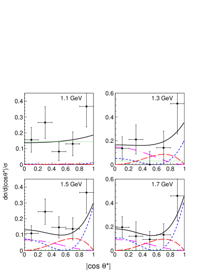
Figure 14: $|\cos\theta^{*}|$ dependence of the normalized differential cross sections and the fitted results in the four $W$ bins indicated in each panel. The lines shown are obtained from the nominal fit (at $\langle Q^{2}\rangle=6.5~{}{\rm GeV}^{2}$). Black solid lines show the total, green dotted the $|S|^{2}$ term, blue dashed the $|D_{0}|^{2}$ term, red long-dashed the $|D_{1}|^{2}$ term, and magenta dash-dotted the $|D_{2}|^{2}$ term.

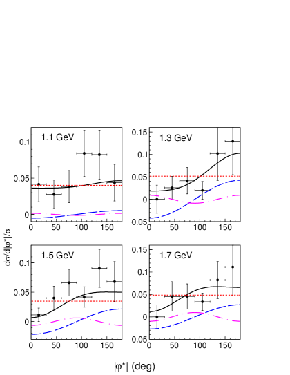
Figure 15: $|\varphi^{*}|$ dependence of the normalized differential cross sections and the fitted results in the four $W$ bins indicated in each panel. The lines shown result from the nominal fit (at $\langle Q^{2}\rangle=6.5~{}{\rm GeV}^{2}$). Black solid line: total, red dotted: $t_{0}$; blue dashed: $t_{1}\cos|\varphi^{*}|$; and magenta dash-dotted: $t_{2}\cos 2|\varphi^{*}|$.

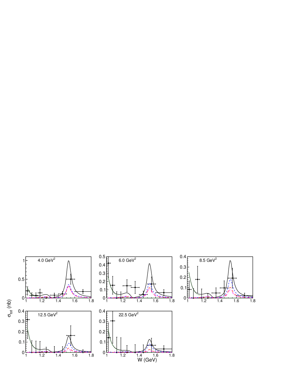
Figure 16: Total cross sections (integrated over angle) for $\gamma^{*}\gamma\to K^{0}_{S}K^{0}_{S}$ in five $Q^{2}$ bins as indicated in each panel, together with the fit results described in VI.3. Black solid line: total; green dotted: $|S|^{2}$; blue dashed: $|D_{0}|^{2}$; red long-dashed: $|D_{1}|^{2}$; and magenta dash-dotted: $|D_{2}|^{2}$.

Table 7: Transition form factors of the $f_{2}^{\prime}(1525)$ meson ($\times 10^{-2}$) for each helicity and combined. The first and second uncertainties are statistical and systematic, respectively. The normalization of the TFF is such that $F_{f2p}(0)=1$. There is an additional overall systematic uncertainty of $\pm 7\%$ due to the error in the tabulated two-photon decay width $\Gamma_{\gamma\gamma}$ of the $f_{2}^{\prime}(1525)$ state.

$\overline{Q}^{2}({\rm GeV}^{2})$	helicity-0	helicity-1	helicity-2	Total
3.51	$15.8^{+2.4}_{-2.5}$${}^{+4.1}_{-5.1}$	$10.6^{+1.9}_{-2.0}$${}^{+2.8}_{-7.3}$	$14.8^{+3.3}_{-3.6}$${}^{+4.1}_{-6.6}$	$24.1^{+2.6}_{-2.5}$${}^{+6.0}_{-8.2}$
5.87	$9.7^{+2.0}_{-2.0}$${}^{+2.2}_{-3.6}$	$5.8^{+1.3}_{-1.4}$${}^{+1.3}_{-4.2}$	$7.3^{+2.1}_{-2.3}$${}^{+1.8}_{-3.7}$	$13.4^{+2.6}_{-2.5}$${}^{+3.0}_{-5.2}$
8.30	$8.6^{+1.8}_{-1.8}$${}^{+1.7}_{-1.2}$	$4.7^{+1.1}_{-1.1}$${}^{+1.0}_{-3.0}$	$5.4^{+1.6}_{-1.9}$${}^{+1.3}_{-2.1}$	$11.2^{+2.3}_{-2.2}$${}^{+2.2}_{-1.8}$
12.1	$5.1^{+1.7}_{-1.6}$${}^{+2.1}_{-0.0}$	$2.6^{+0.9}_{-0.8}$${}^{+1.1}_{-1.6}$	$2.7^{+1.1}_{-1.2}$${}^{+1.2}_{-1.0}$	$6.3^{+2.1}_{-1.9}$${}^{+2.6}_{-0.3}$
20.6	$3.9^{+1.7}_{-1.5}$${}^{+1.2}_{-0.9}$	$1.7^{+0.7}_{-0.7}$${}^{+0.5}_{-1.1}$	$1.6^{+0.8}_{-0.8}$${}^{+0.5}_{-0.7}$	$4.6^{+1.9}_{-1.7}$${}^{+1.4}_{-1.0}$

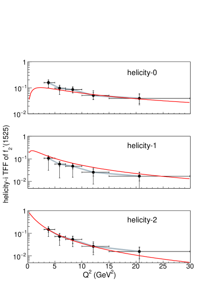
Figure 17: The obtained helicity-0, -1, and -2 TFF of the $f_{2}^{\prime}(1525)$ meson as a function of $Q^{2}$, assuming Eq. (24). Short (long) vertical bars indicate statistical (combined statistical and systematic) errors. The shaded band corresponds to the overall uncertainty arising from the known errors on $\Gamma_{\gamma\gamma}$. The solid line shows the predicted $Q^{2}$ dependence in SBG schuler .

VI.4 Estimation of systematic uncertainties of the TFF

In this subsection, we estimate systematic uncertainties for the TFF of the $f_{2}^{\prime}(1525)$ meson. These arise primarily from the overall $\pm 7$% normalization uncertainty on $\Gamma_{\gamma\gamma}$ that affects all $Q^{2}$ bins uniformly and the individual uncertainties that vary in each $Q^{2}$ bin. The individual systematic uncertainties evaluated below are converted to uncertainties in the helicity-0, -1, and -2 components of the TFF of the $f_{2}^{\prime}(1525)$ meson as summarized in Table 7 and shown in Fig. 17. All uncertainties are summed quadratically in each $Q^{2}$ bin to obtain the total systematic error in that bin.

Individual uncertainties are estimated for the TFF as follows. The uncertainties of the normalization factor in the differential cross sections are estimated by shifting the value corresponding to 1$\sigma$ of the fit. The systematic uncertainties of the measured total cross sections are taken into account by refitting the cross sections with the error shifted. The properties such as the mass, the width, and the branching fraction to $K\bar{K}$ of the $f_{2}(1270)$, the $a_{2}(1320)$, and the $f_{2}^{\prime}(1525)$ mesons are shifted by the uncertainties given in the PDG pdg2016 . The $m_{0}^{2}$ in $A_{BW}$ is changed to $(1.0\pm 0.5)~{}{\rm GeV}^{2}$. For $B_{Di}$, they are turned on individually and their effects are taken as uncertainties.

Systematic uncertainties due to various possible distortions in the distributions of $W$, $Q^{2}$, $|\cos\theta^{*}|$, and $|\varphi^{*}|$ studied below are evaluated parametrically. The effect of a shift of $\pm 10$% in the total and the differential cross sections over the full range of $W$ is estimated by multiplying the cross sections by [$1\pm 0.25\times(W-1.4~{}{\rm GeV})$]. The effect of a shift of $\pm 5$% in the total cross sections over the full range of $Q^{2}$ is evaluated by multiplying by [$1\pm 0.006\times(Q^{2}-12.2~{}{\rm GeV}^{2})$]. Additional uncertainties considered are those arising from changing the range of $W$, from $1.0-1.8$ to $1.0-2.0$ or $1.0-1.6$ GeV. The effect of a shift of $\pm 10$% in the differential cross sections as a function of $\cos\theta^{*}$ is evaluated by multiplying by [$1\pm 0.2\times(|\cos\theta^{*}|-0.5)$]. The effect of a shift of $\pm 10$% in the differential cross sections as a function of $|\varphi^{*}|$ is evaluated by multiplying by [$1\pm 0.0011\times(|\varphi^{*}|-90^{\circ})$]. The uncertainty in the convex or concave shape of $\cos\theta^{*}$ is evaluated by multiplying by [$1.1-0.8\times(|\cos\theta^{*}|-0.5)^{2}$], or [$0.9+0.8\times(|\cos\theta^{*}|-0.5)^{2}$], respectively. Similarly, the uncertainty in the convex or concave shape of $|\varphi^{*}|$ is evaluated by multiplying by [$1.1-2.5\times 10^{-5}\times(|\varphi^{*}|-90^{\circ})^{2}$] or [$0.9+2.5\times 10^{-5}\times(|\varphi^{*}|-90^{\circ})^{2}$], respectively.

VI.5 $Q^{2}$ dependence of cross sections near the $K^{0}_{S}K^{0}_{S}$ threshold

In the $\gamma\gamma\rightarrow K^{0}_{S}K^{0}_{S}$ reaction, a peak structure near $K^{0}_{S}K^{0}_{S}$ threshold is expected, based on a comprehensive amplitude analysis using the data of $\gamma\gamma\rightarrow\pi\pi$ and $K\bar{K}$ Pennington . In Refs. achasov1 and achasov2 , it is predicted that this peak structure persists even if the $f_{0}(980)$ and the $a_{0}(980)$ mesons interfere destructively. Experimentally, there have been no measurements to date of the two-photon cross section in the energy region of $W$ below $1.05~{}{\rm GeV}$.

The nominal fit shows that S wave can be expressed by a Breit-Wigner function with a mass of 0.995 GeV/$c^{2}$. Motivated by this, we have plotted the $Q^{2}$ dependence of the total cross sections in the energy bins at 1.023 GeV, 1.075 GeV, and 1.125 GeV as shown in Fig. 18. We also show the $Q^{2}$ dependence for a $J^{P}=0^{+}$ state predicted with $M=0.98~{}{\rm GeV}/c^{2}$ in SBG schuler normalized by the points at $Q^{2}=0$, which are translated from the data of the no-tag measurement of this process ksks assuming an isotropic angular dependence. These data are available at the two higher-$W$ regions. The measured cross sections are slightly larger than the predicted values, though not inconsistent with them given the large statistical errors. The cross sections increase as $W$ approaches the mass threshold, which may signify the threshold enhancement suggested in Ref. Pennington .

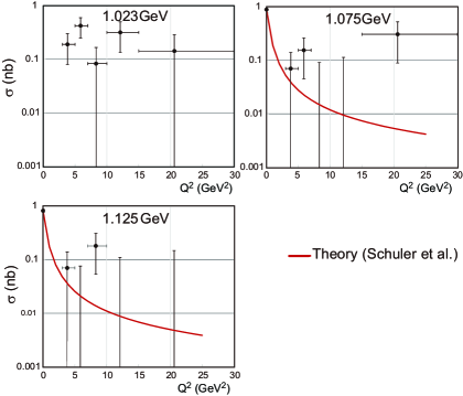
Figure 18: $Q^{2}$ dependence of the cross section in the three $W$ regions near the $K^{0}_{S}K^{0}_{S}$ mass threshold, with central values as indicated in the subpanels. Only statistical errors are shown. Solid curves show the predicted $Q^{2}$ dependence in SBG schuler

.

VII Summary and Conclusion

We have measured the cross section of $K^{0}_{S}$-pair production in single-tag two-photon collisions, $\gamma^{*}\gamma\to K^{0}_{S}K^{0}_{S}$ up to $Q^{2}=30~{}{\rm GeV}^{2}$ based on a data sample of 759 fb^-1 collected with the Belle detector at the KEKB asymmetric-energy $e^{+}e^{-}$ collider. The data covers the kinematic range $1.0~{}{\rm GeV}<W<2.6~{}{\rm GeV}$ and the angular range of $|\cos\theta^{*}|<1.0$ and $0\leq|\varphi^{*}|\leq 180^{\circ}$ in the $\gamma^{*}\gamma$ c.m. system.

For the first time, we find the $f_{2}^{\prime}(1525)$, $\chi_{c0}(1P)$, and $\chi_{c2}(1P)$ mesons in high-$Q^{2}$ $\gamma^{*}\gamma$ scattering. These resonances are most visible in the corresponding no-tag mode ksks .

We have estimated the $\chi_{c0}$ and $\chi_{c2}$ partial decay widths $\Gamma_{\gamma*\gamma}$ as a function of $Q^{2}$. The $Q^{2}$ dependences of $\Gamma_{\gamma*\gamma}$ are normalized to $\Gamma_{\gamma\gamma}$ at $Q^{2}=0$ and compared with SBG schuler , as shown in Fig. 13. They are in agreement, albeit with very limited statistics.

A partial-wave analysis has also been conducted for the $\gamma^{*}\gamma\to K^{0}_{S}K^{0}_{S}$ event sample. The helicity-0, -1, and -2 transition form factors (TFFs) of the $f_{2}^{\prime}(1525)$ meson are measured for the first time for $Q^{2}$ up to $30~{}{\rm GeV}^{2}$ and are compared with theoretical predictions. The measured helicity-0 and -2 TFFs of the $f_{2}^{\prime}(1525)$ meson agree well with SBG schuler , and the helicity-1 TFF is not inconsistent with prediction.

We have also compared the total cross section near the $K^{0}_{S}K^{0}_{S}$ mass threshold as a function of $Q^{2}$ with the prediction for a $J^{P}=0^{+}$ state with $M=0.98~{}{\rm GeV}/c^{2}$ in SBG schuler , although our limited statistics currently preclude a conclusive interpretation.

References

(1)
H. Kawamura and S. Kumano,
Phys. Rev. D 89, 054007 (2014).
(2)
G. Colangelo, M. Hoferichter, M. Procura and P. Stoffer,
J. High Energy Physics 1409, 091 (2014).
(3)
G. Colangelo, M. Hoferichter, B. Kubis, M. Procura and P. Stoffer,
Phys. Lett. B 738, 6 (2014).
(4)
M. Masuda et al. (Belle Collaboration),
Phys. Rev. D 93, 032003 (2016).
(5)
I. F. Ginzburg, A. Schiller, and V. G. Serbo,
Eur. Phys. J. C 18, 731 (2001);
V.G. Serbo (private communication).
(6)
G. A. Schuler, F. A. Berends, and R. van Gulik,
Nucl. Phys. B 523, 423 (1998).
(7)
S. Uehara et al. (Belle Collaboration),
Prog. Theor. Exp. Phys. 2013, 123C01 (2013).
(8)
A. Abashian et al. (Belle Collaboration),
Nucl. Instrum. Methods Phys. Res., Sect. A 479, 117 (2002).
(9)
J. Brodzicka et al. (Belle Collaboration),
Prog. Theor. Exp. Phys. 2012, 04D001 (2012).
(10)
S. Kurokawa and E. Kikutani, Nucl. Instrum. Methods Phys. Res., Sect. A 499, 1 (2003),
and other papers included in this volume.
(11)
T. Abe et al., Prog. Theor. Exp. Phys. 2013, 03A003 (2013).
(12)
B. G. Cheon et al., Nucl. Instrum. Methods Phys. Res., Sect. A 494, 548 (2002).
(13)
S. Uehara, KEK-Report 96-11, arXiv:1310.0157 [hep-ph] (1996).
(14)
R. Brun et al., Report No. CERN DD/EE/84-1, 1987.
(15)
C. Patrignani et al. (Particle Data Group),
Chin. Phys. C 40, 100001 (2016).
(16)
S. Uehara et al. (Belle Collaboration),
Phys. Rev. D 86, 092007 (2012).
(17)
J. J. Sakurai,
Phys. Rev. Lett. 22, 981 (1969).
(18) We denote individual partial
waves by upright letters and parameterized waves by italics.
(19)
V. Pascalutsa, V. Pauk, and M. Vanderhaeghen,
Phys. Rev. D 85, 116001 (2012).
(20) L. Y. Dai, and M. R. Pennington,
Phys. Rev. D 90, 036004 (2014).
(21)
See the review by S. Baker and R. D. Cousins,
Nucl. Instrum. Methods Phys. Res. 221, 437 (1984).
(22)
N. N. Achasov and G. N. Shestakov, Phys. Usp. 54, 799 (2011).
(23)
N. N. Achasov and G. N. Shestakov, JETP Lett. 96, 493 (2012).