3D non-Fermi liquid behavior from 1D quantum critical local moments

Laura Classen, Igor Zaliznyak, and Alexei M. Tsvelik Condensed Matter Physics and Materials Science Division, Brookhaven National Laboratory, Upton, NY 11973-5000, USA
Abstract

We study the temperature dependence of the electrical resistivity in a system composed of critical spin chains interacting with three dimensional conduction electrons and driven to criticality via an external magnetic field. The relevant experimental system is Yb2Pt2Pb, a metal where itinerant electrons coexist with localized moments of Yb-ions which can be described in terms of effective $S=1/2$ spins with dominantly one-dimensional exchange interaction. The spin subsystem becomes critical in a relatively weak magnetic field, where it behaves like a Luttinger liquid. We theoretically examine a Kondo lattice with different effective space dimensionalities of the two interacting subsystems. We characterize the corresponding non-Fermi liquid behavior due to the spin criticality by calculating the electronic relaxation rate and the $dc$ resistivity and establish its quasi linear temperature dependence.

Coexistence of conduction electrons and localized magnetic moments leads to fascinating physics driven by a competition between screening of the magnetic moments by the conduction electrons, and strong correlations from interaction between the moments. This competition plays itself differently depending on such factors as symmetry, crystal structure, disorder and space dimensionalitybrandt1984 ; lee1986 ; stewart2001 ; gegenwart2008 ; wirth2016 . Prototypical materials for the study of this interplay are rare earth based metals containing a band of conduction electrons and localized moments of strongly correlated $f$-electrons stewart1984 . If the Kondo screening wins, the low energy sector behaves like a Fermi liquid of heavy quasiparticles. It is usually assumed that he opposite case characterized by a strong interspin interaction leads to magnetic ordering and decoupling of the two subsystems doniach1977 . Such a scenario, however, is likely to be substantially modified in the case when the spin subsystem is quasi one dimensional and hence cannot order by itselfcoleman2010 . This is exactly the case we are interested in.

In our considerations, we have been motivated by experiments on Yb2Pt2Pb, a metallic compound, where the itinerant electrons originate from Pt and Pb ions and the local moments are formed by electrons localized on the orbitals of 4f13 Yb ionspoettgen . In the crystal field, these moments are reduced to the lowest $j=\pm 7/2$ Kramers doubletskim2008 ; ochiai2011 . There are several features making Yb2Pt2Pb very special. The local moments form a quasi one-dimensional subsystem of effective spins S=1/2 weakly interacting with three dimensional (3D) conduction electrons. As was found in we , the magnetic excitations are strongly incoherent, gapped (see also miiller ) and essentially one dimensional in zero magnetic field. The Ising-like chain is already ordered at $T=0$ and the effect of the small inter-chain coupling (of primarily dipolar origin) is simply to extend this order to finite temperatures ย  2K miiller without noticeably changing the magnitude of the order parameter we . The exchange interaction with the conduction electrons appears to be weak, with no experimental indication of Kondo screening kim2013 , particularly in zero magnetic field when the spectrum is gapped. However, when the field overcomes the gap, the magnetic excitations become critical and the 3D magnetic order is strongly suppressed miiller ,unpublished . Then their interaction with the conduction electrons becomes important ref . The strongest critical fluctuations of one dimensional magnetic chains embedded in a 3D host are centered not at one wave vector, but on an entire plane in 3D reciprocal space. As a consequence, scattering of electrons with critical fluctuations is strong not just at certain spots, but over a continuum manifold, making a significant portion of the Fermi surface โ€œhotโ€. Hence, we expect a regime with non-Fermi-liquid (NFL) behavior, which persists until the magnetic field exceeds an upper critical threshold, where the magnetization saturates and the excitation spectrum becomes gapped again. Interestingly, the critical behavior is due to local moments that are coupled to, but not hybridized with itinerant electrons. Furthermore, it appears in the unique situation of a Kondo lattice where the two interacting subsystems have different effective space dimensionality.

To characterize the emergent NFL behavior, we perturbatively calculate the leading frequency and temperature dependence of the electronic relaxation rate and $dc$ conductivity. They are strongly affected by the scattering of electrons on the critical modes of the Yb spin subsystem. As an advantage of the one-dimensionality, the exact form of the low energy asymptotics of the spin-spin correlation functions is known so that we can account for the non-trivial dynamics of the local moments in a clear, analytical way. We discover a distinct NFL signature in both, conductivity and relaxation rate, induced by the staggered part of the correlations among local moments. In contrast, the contribution from the uniform component is subleading. In particular, we find that for an extended magnetic field regime, the resistivity scales linearly with temperature. This anomalous temperature dependence exists for all current directions, parallel or perpendicular to the Yb-chains. However, we find that the absolute value of the resistivity parallel to the chains is markedly smaller than the one perpendicular to them due to the one dimensional character of the spin excitations. This agrees with the experimental measurements for Yb2Pt2Pb, which show an anisotropic resistivity linear in $T$ at intermediate magnetic fieldsmiiller ; unpublished .

Model The neutron-scattering experiments in Yb2Pt2Pb can be described by a model of weakly-interacting, anisotropic spin S=1/2 chains we in terms of exact expressions of the XXZ spin-1/2 chain Hamiltonian with moderate Ising anisotropy leading to a small excitation gap $\Delta$. Here, we will study the situation when this gap closes due to an external magnetic field and the spins enter a Luttinger liquid phase. Due to the dipolar origin of the interchain coupling its effect in the absence of order becomes negligible miiller ; unpublished . The low-energy spin-spin correlation functions take a universal form and do not depend on the exact microscopic model. The only remaining memory is contained in the correlation function exponents as shown below.

Critical modes appear at different wavevectors $Q$, corresponding to the uniform and staggered components of the correlation functions chitra1997 ; giamarchibook ; alexeibook ; lecturenotes . For correlations parallel to the spin $z$-direction, $\langle S^{z}(\omega,q)S^{z}(0,0)\rangle$, they are around $Q=0$ and $Q=\pi(1\pm 2M)$, where $M\ll 1$ is the induced magnetization, $M\propto\sqrt{h-\Delta}$, due to the magnetic field $h=g\mu_{b}H$. Critical $\langle S^{+}(\omega,q)S^{-}(0,0)\rangle$ modes appear close to $Q=\pm 2\pi M$ and $Q=\pi$. The zero-temperature dynamical susceptibility corresponding to the uniform and staggered correlation functions for the $S^{z}$ components takes the form

$\displaystyle\chi_{zz}^{u}(i\omega,q_{\|})$ $\displaystyle=\chi_{zz,0}^{u,0}\frac{q_{||}^{2}}{\omega^{2}+v_{s}^{2}q_{||}^{2}}$ (1)
ฯ‡zโ€‹zsโ€‹(iโ€‹ฯ‰,qโˆฅ)superscriptsubscript๐œ’๐‘ง๐‘ง๐‘ ๐‘–๐œ”subscript๐‘žโˆฅ\displaystyle\chi_{zz}^{s}(i\omega,q_{\|}) $\displaystyle=\chi_{zz}^{s,0}\frac{1}{(\omega^{2}+v_{s}^{2}q_{||}^{2})^{1-K}}$ (2)

where $q$ measures the deviation from the critical wavevector $Q$ and the parameters label spin excitation velocity vssubscript๐‘ฃ๐‘ v_{s} and effective Luttinger liquid parameter $K$. The corresponding $S^{+}S^{-}$ correlations are given by

$\displaystyle\chi_{+-}^{u}(i\omega,q_{\|})$ $\displaystyle=\chi_{+-}^{u,0}\frac{-\omega^{2}+v_{s}^{2}q^{2}}{(\omega^{2}+v_{s}^{2}q_{||}^{2})^{2-K-1/(4K)}}$ (3)
ฯ‡+โˆ’sโ€‹(iโ€‹ฯ‰,qโˆฅ)superscriptsubscript๐œ’absent๐‘ ๐‘–๐œ”subscript๐‘žโˆฅ\displaystyle\chi_{+-}^{s}(i\omega,q_{\|}) $\displaystyle=\chi_{+-}^{s,0}\frac{1}{(\omega^{2}+v_{s}^{2}q_{||}^{2})^{1-1/(4K)}}$ (4)

where $\chi_{+-}/2=\chi_{xx}=\chi_{yy}$ due to spin rotation symmetry around the external magnetic field. The Luttinger liquid parameter $K$ varies with magnetic field and depends on the microscopic model. For the XXZ spin-1/2 chain, it takes values between $K=1/4$ and $1$, but is close to $K=1/2$ for an extended regime okunishi2007 . In summary, the spin action becomes

Ss=โˆ‘i=x,y,zโˆ‘ฮฑ=u,sTโ€‹โˆ‘iโ€‹ฯ‰โˆซpSiฮฑโ€‹[ฯ‡iฮฑ]โˆ’1โ€‹Siฮฑ.subscript๐‘†๐‘ subscript๐‘–๐‘ฅ๐‘ฆ๐‘งsubscript๐›ผ๐‘ข๐‘ ๐‘‡subscript๐‘–๐œ”subscript๐‘subscriptsuperscript๐‘†๐›ผ๐‘–superscriptdelimited-[]subscriptsuperscript๐œ’๐›ผ๐‘–1subscriptsuperscript๐‘†๐›ผ๐‘–S_{s}=\sum_{i=x,y,z}\sum_{\alpha=u,s}T\sum_{i\omega}\int_{p}S^{\alpha}_{i}[\chi^{\alpha}_{i}]^{-1}S^{\alpha}_{i}. (5)

where $\int_{p}=\int d^{3}p/(2\pi)^{3}$ and $T\sum_{i\omega}$ is a summation over Matsubara frequencies. For the array of noninteracting chains the spin susceptibility does not depend on the perpendicular momenta, i.e. $\chi_{i}^{\alpha}(p_{\|},p_{\perp})=\chi(p_{\|})$.

The electronic part is assumed to be well described by free electrons in a magnetic field, since the material is an excellent metal

Sฯˆ=Tโ€‹โˆ‘iโ€‹ฯ‰โˆซp(iโ€‹ฯ‰โˆ’ฮพpโ€‹ฯƒ)โ€‹ฯˆp,ฯƒโ€ โ€‹ฯˆp,ฯƒ.subscript๐‘†๐œ“๐‘‡subscript๐‘–๐œ”subscript๐‘๐‘–๐œ”subscript๐œ‰๐‘๐œŽsubscriptsuperscript๐œ“โ€ ๐‘๐œŽsubscript๐œ“๐‘๐œŽS_{\psi}=T\sum_{i\omega}\int_{p}(i\omega-\xi_{p\sigma})\psi^{\dagger}_{p,\sigma}\psi_{p,\sigma}. (6)

The dispersion relation $\xi_{p,\sigma}=p^{2}/(2m)-\mu_{\sigma}$ accounts for the Zeeman splitting modeled by the spin-dependent chemical potential $\mu_{\sigma}=\mu-\sigma h$ with $\sigma=\pm$. This defines the Fermi vectors $p_{F\sigma}=\sqrt{2m\mu_{\sigma}}$ and $p_{F}=\sqrt{2m\mu}$. We will label the directions perpendicular and parallel to the local spin chains by ${\boldsymbol{p}}_{\perp}$ and $p_{\|}$. Both descriptions for electrons and spins are only valid up to a momentum cutoff $\Lambda$.

We model the coupling of the quasi one-dimensional spinons in the Yb-chains to the 3D electrons as

Sc=Jโ€‹T2โ€‹โˆ‘iโ€‹k0,iโ€‹k0โ€ฒโˆซkโˆซkโ€ฒV๐’Œโ€‹ฯƒโˆ—โ€‹V๐’Œโ€ฒโ€‹ฯƒโ€ฒโ€‹ฯˆkโ€‹ฯƒโ€ โ€‹๐ˆฯƒโ€‹ฯƒโ€ฒโ€‹ฯˆkโ€ฒโ€‹ฯƒโ€ฒโ€‹๐‘บโ€‹(kโˆ’kโ€ฒ)subscript๐‘†๐‘๐ฝsuperscript๐‘‡2subscript๐‘–subscript๐‘˜0๐‘–superscriptsubscript๐‘˜0โ€ฒsubscript๐‘˜subscriptsuperscript๐‘˜โ€ฒsubscriptsuperscript๐‘‰๐’Œ๐œŽsubscript๐‘‰superscript๐’Œโ€ฒsuperscript๐œŽโ€ฒsubscriptsuperscript๐œ“โ€ ๐‘˜๐œŽsubscript๐ˆ๐œŽsuperscript๐œŽโ€ฒsubscript๐œ“superscript๐‘˜โ€ฒsuperscript๐œŽโ€ฒ๐‘บ๐‘˜superscript๐‘˜โ€ฒS_{c}=JT^{2}\sum_{ik_{0},ik_{0}^{\prime}}\int_{k}\int_{k^{\prime}}V^{*}_{{\boldsymbol{k}}\sigma}V_{{\boldsymbol{k}}^{\prime}\sigma^{\prime}}\psi^{\dagger}_{k\sigma}{\boldsymbol{\sigma}}_{\sigma\sigma^{\prime}}\psi_{k^{\prime}\sigma^{\prime}}{\boldsymbol{S}}(k-k^{\prime}) (7)

The coupling $J$ is small and only weakly hybridizes the conduction electrons and the spins. The matrix elements are given by the overlaps of the plane waves of conduction electrons with the wave functions of the $f$-electrons, which are described by the effective spins $S=1/2$. The $f$-electron wave functions are spherical harmonics with angular momentum $L=3,J=7/2$ and $m_{L}=\pm 3$. Their spacial parts are $V_{{\boldsymbol{k}}\pm}=Y_{3,\pm 3}\left({\boldsymbol{k}}/k\right)\sim(k_{\|}\pm ik_{\perp,1})^{3}/{k^{3}}$ with ${\boldsymbol{k}}_{\perp}=(k_{\perp,1},k_{\perp,2})^{T}$. In these notations, the quantization axis of the Yb moments is along $k_{\perp,2}$.

In summary, the action becomes S=Ss+Sฯˆ+Sc๐‘†subscript๐‘†๐‘ subscript๐‘†๐œ“subscript๐‘†๐‘S=S_{s}+S_{\psi}+S_{c}. The model is similar to a generalized spin-fermion model, however, in our case spins disperse only in one direction and they are independent degrees of freedom with non-trivial dynamics inherited from their local character.

Refer to caption
Refer to caption
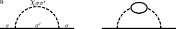
Figure 1: (a) Diagrammatic representation of the correction to the electron self-energy without and with renormalized spin propagator. (b) Dyson equation for the current vertex. The empty (black) triangle with the attached dotted line denotes the bare (full) current vertex. Solid (dashed) lines are electron (spin) propagators.

Non-Fermi-liquid regime The scattering between electrons and spinons leads to remarkable modifications in their correlation functions. In particular, as we will demonstrate, it can destroy the Fermi liquid character of the conduction electrons. The corresponding information is encoded in the imaginary part of the electron self-energy - the relaxation rate. The general form of the one-loop electron self-energy is shown in Fig.ย 1 and reads $\Sigma_{\sigma}(i\omega,{\boldsymbol{k}})=J^{2}\sum_{i,\alpha}T\sum_{i\nu}\int_{q}|V_{k\sigma}|^{2}|V_{k+q\sigma^{\prime}}|^{2}\chi_{i}^{\alpha}(i\nu,q_{\|})G_{\sigma^{\prime}}(i\omega+i\nu,{\boldsymbol{k}}+{\boldsymbol{q}})$ with the bare electron propagator $G_{\sigma}^{-1}(i\omega,k)=i\omega-\xi_{{\boldsymbol{k}}\sigma}$. In principle, we have to sum over all critical spin modes $\chi_{i}^{\alpha}$ in this expression, but we found that the leading contribution comes from the staggered modes (ฯ‡zโ€‹zssuperscriptsubscript๐œ’๐‘ง๐‘ง๐‘ \chi_{zz}^{s} and ฯ‡+โˆ’ssuperscriptsubscript๐œ’absent๐‘ \chi_{+-}^{s}) and we will focus on them in the following. The one-loop self-energy due to the uniform modes is given in the supplemental material (SM).

A special feature of our model is that due to the one dimensional character of the spin excitations these staggered modes affect a significant part of the FS. The dominant contribution to the self-energy on the FS comes from states, where the propagators G๐บG and ฯ‡๐œ’\chi are singular, i.e. k๐‘˜k and k+q๐‘˜๐‘žk+q are close to the FS and q๐‘žq is close to Q๐‘„Q. Typically for large Q๐‘„Q, only small parts of the FS become โ€œhotโ€ so that their effect is limited. But due to the one-dimensional spin excitations,
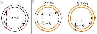
 only the parallel component qโˆฅโ‰ˆQsubscript๐‘žโˆฅ๐‘„q_{\|}\approx Q is restricted in our case and we can use the perpendicular component qโŸ‚subscript๐‘žperpendicular-toq_{\perp} to reach a final state on the FS. This defines an entire continuum manifold of hot states on the FS. The mechanism is sketched in Fig.ย 2.

Refer to caption
Figure 2: (a) If spin and electron correlations are both three dimensional, only a few hot spots or lines appear (colored bright points), where the initial state $k$ and the final state $k+Q$ are both at the FS. (b) If spins are quasi one dimensional and electrons three dimensional a significant part of the FS is hot (colored bright part in the sketch). The reason is that for almost every initial $k$ on the FS, one can find a final $k+q$ that is also on the FS due to the free choice of $q_{\perp}$. For a spherical FS, it depends on the ratio $Q/k_{F}$ which part of the FS is hot. If $Q<k_{F}$ the whole FS is hot.

In the following, we will be interested in the frequency dependence of the self-energy. It is thus sufficient to consider the FS-averaged relaxation rate

$\displaystyle\Gamma_{\sigma}(\omega)=-\int_{p}\frac{\delta(\xi_{{\boldsymbol{p}}\sigma})}{N_{\sigma}}{\text{Im}\Sigma}^{R}_{\sigma}(\omega,{\boldsymbol{p}}),$ (8)

with the retarded self-energy $\Sigma^{R}(\omega,{\boldsymbol{p}})$ and the density of states at the $\sigma$-FS $N_{\sigma}=p_{F\sigma}m/(2\pi^{2})$.

The resulting FS-averaged relaxation rate due to scattering with staggered spin modes is

$$\Gamma_{\sigma}(\omega)\approx N_{\sigma}C_{\sigma\sigma}\omega^{2K}+N_{\bar{\sigma}}C_{\sigma\bar{\sigma}}\omega^{\frac{1}{2K}}$$ (9)

with $\bar{\sigma}=-\sigma$ and the prefactors including the averaged coupling Cฯƒโ€‹ฯƒโ€ฒ=ฯ‡ฯƒโ€‹ฯƒโ€ฒ0โ€‹sinโก(ฮณฯƒโ€‹ฯƒโ€ฒโ€‹ฯ€)vsโ€‹(1โˆ’ฮณฯƒโ€‹ฯƒโ€ฒ)โ€‹V2^subscript๐ถ๐œŽsuperscript๐œŽโ€ฒsuperscriptsubscript๐œ’๐œŽsuperscript๐œŽโ€ฒ0subscript๐›พ๐œŽsuperscript๐œŽโ€ฒ๐œ‹subscript๐‘ฃ๐‘ 1subscript๐›พ๐œŽsuperscript๐œŽโ€ฒ^superscript๐‘‰2C_{\sigma\sigma^{\prime}}=\frac{\chi_{\sigma\sigma^{\prime}}^{0}\sin(\gamma_{\sigma\sigma^{\prime}}\pi)}{v_{s}(1-\gamma_{\sigma\sigma^{\prime}})}\widehat{V^{2}} and $\widehat{V^{2}}=J^{2}\int_{p}\int_{q}\frac{\delta(\xi_{\sigma p})\delta(\xi_{\sigma^{\prime}p+q+Q_{\sigma\sigma^{\prime}}})}{N_{\sigma}N_{\sigma^{\prime}}}|V_{\sigma p}|^{2}|V_{\sigma^{\prime}p+q+Q_{\sigma\sigma^{\prime}}}|^{2}$. In this notation, $\chi_{\sigma\sigma}=\chi_{zz}$, $\chi_{\sigma\bar{\sigma}}=\chi_{+-}$ and $\gamma_{\sigma\sigma}=1-K$, $\gamma_{\sigma\bar{\sigma}}=1-1/(4K)$. Details of the calculation are given in the SM. We find that the scaling of the averaged relaxation rate depends on the Luttinger parameter $K$, which varies with the magnetic field.

Additionally, we can include the electron dynamics into the spin susceptibility and compute the electron self-energy with the renormalized spin propagator (see Fig.ย 1). In contrast to the โ€œconventionalโ€ spin-fermion model, the spins in our heavy-fermion system are independent degrees of freedom, not composite quasiparticles from electron-hole excitations. This means that the corrections to the spin susceptibility become important for energies much smaller than the Fermi energy ฯ‰<vsโ€‹ฮ›โ‰ชEF๐œ”subscript๐‘ฃ๐‘ ฮ›much-less-thansubscript๐ธ๐น\omega<v_{s}\Lambda\ll E_{F}. We are, however, interested in exactly this low-energy regime. The electron-renormalized spin propagator becomes ฯ‡โˆ’1โ€‹(ฯ‰,q)=ฯ‡bโ€‹aโ€‹rโ€‹eโˆ’1โ€‹(ฯ‰,q)+ฮ โ€‹(ฯ‰,q)superscript๐œ’1๐œ”๐‘žsubscriptsuperscript๐œ’1๐‘๐‘Ž๐‘Ÿ๐‘’๐œ”๐‘žฮ ๐œ”๐‘ž\chi^{-1}(\omega,q)=\chi^{-1}_{bare}(\omega,q)+\Pi(\omega,q). The real part of the polarization operator ฮ โ€ฒsuperscriptฮ โ€ฒ\Pi^{\prime} is approximately constant. The imaginary part depends on the characteristic momentum transfer mediated by the spins. For large momentum transfers it takes the form abrikosov ฮ โ€‹(ฯ‰,q)โ‰ˆโˆ’ฮ rโˆ’iโ€‹ฯ„๐’’โŸ‚โ€‹ฯ‰,ฮ ๐œ”๐‘žsubscriptฮ ๐‘Ÿ๐‘–subscript๐œsubscript๐’’perpendicular-to๐œ”\Pi(\omega,q)\approx-\Pi_{r}-i\tau_{{\boldsymbol{q}}_{\perp}}\omega, where the momentum-dependence of the imaginary part is mainly due to perpendicular momenta as indicated by the subscript because $q_{\|}\approx Q$. The leading contribution to the electron scattering rate incuding the polarization bubble in the spin correlation functions is then modified to (see SM)

$\displaystyle\Gamma_{\sigma}(\omega)=\sum_{\sigma^{\prime}}N_{\sigma^{\prime}}C_{\sigma\sigma^{\prime}}\omega.$ (10)

We see that, if one takes into account the renormalization of the spin susceptibility by the conduction electrons, the result shows a linear scaling, independent of the value of the Luttinger liquid exponent.

Conductivity The temperature dependence of the resistivity is one of the hallmarks of NFL behavior. In a Fermi liquid, it is typically quadratic with temperature. In contrast, in this section, we show that the resistivity scales linearly with $T$ in the field-induced critical regime Furthermore, since the scattering is caused by the one-dimensional chains, the coefficient of the linear $T$-term turns out to be different for the directions parallel and perpendicular to the chains. For simplicity, we will perform the calculations at zero temperature and assume that the scaling with temperature is the same as the scaling with frequency (see SM).

The $dc$ conductivity can be expressed in terms of the Kubo formula as

$\displaystyle\sigma_{\|/\perp}^{\sigma}\approx$ $\displaystyle\frac{6e^{2}n_{\sigma}}{c_{\|/\perp}m}\int\frac{d\epsilon}{2\pi}\left(-\frac{dn_{F}}{d\epsilon}\right)\frac{\gamma_{\sigma}^{\|/\perp}(\epsilon)}{\Gamma_{\sigma}(\epsilon)}$ (11)

with $c_{i}=1+\delta_{i,\perp}$ and the number density $n_{\sigma}=p_{F\sigma}^{3}/(6\pi^{2})$. $\gamma_{\sigma}$ denotes the scalar part of the current vertex ${\boldsymbol{\Gamma}}^{\sigma}={\boldsymbol{p}}\gamma_{\sigma}$ and we define its FS-average for the different directions $\gamma_{\sigma}^{\|/\perp}(\epsilon)=\frac{1}{N_{\sigma}}\int_{p}\frac{p_{\|/\perp}^{2}}{p^{2}}\delta(\xi_{\sigma{\boldsymbol{p}}})\gamma_{\sigma}({\boldsymbol{p}},\epsilon-i0^{+},\epsilon+i0^{+})$. Their sum, in turn, is the average of the scalar current vertex $\gamma_{\sigma}(\epsilon)=\gamma^{\|}_{\sigma}(\epsilon)+\gamma^{\perp}_{\sigma}(\epsilon)=\frac{1}{N_{\sigma}}\int_{p}\delta(\xi_{\sigma{\boldsymbol{p}}})\gamma_{\sigma}({\boldsymbol{p}},\epsilon-i0^{+},\epsilon+i0^{+})$. The approximations used here and in the following are explained in the SM. They only affect prefactors, but lead to the correct scaling behavior bharadwaj2014 ; belitz2010 .

For the correct scaling of the conductivity, vertex corrections are usually important because they weight the scattering events appropriately Mahan . The vertex corrections can be determined from the Dyson equation for the current vertex, whose diagrammatic representation is shown in Fig.ย 1. This leads to

$\displaystyle{\boldsymbol{p}}_{i}^{2}$ $\displaystyle\gamma_{\sigma}({\boldsymbol{p}},ip,ip+i\omega)$
$\displaystyle={\boldsymbol{p}}_{i}^{2}+J^{2}\sum_{\sigma^{\prime}}T\sum_{iq}\int_{q}|V(p)|^{2}|V(q)|^{2}\chi_{\sigma\sigma^{\prime}}(iq-ip,{\boldsymbol{q}}-{\boldsymbol{p}})$
$\displaystyle\times G(iq,{\boldsymbol{q}})G(iq+i\omega,{\boldsymbol{q}}){\boldsymbol{p}}_{i}{\boldsymbol{q}}_{i}\gamma_{\sigma^{\prime}}({\boldsymbol{q}},iq,iq+i\omega)$ (12)

with $i=\|,\perp$. The resulting scalar current vertex is constant to the leading order:

$\displaystyle\gamma_{\sigma}$ $\displaystyle\approx\frac{1}{1-f}+\mathcal{O}(h/E_{F}),$ (13)

with $f=1-Q^{2}/(2p_{F}^{2})+\mathcal{O}(h/E_{F})$ and we have neglected terms of order of the magnetic field over the Fermi energy $h/E_{F}\ll 1$. The full expression is given in the SM. As used before, $Q$ is the typical momentum transfer parallel to the chains. To estimate the relative magnitude of $\gamma_{\sigma}^{\|}$ and $\gamma_{\sigma}^{\perp}$, we solve Eq.ย (3D non-Fermi liquid behavior from 1D quantum critical local moments) for $\gamma_{\sigma}^{\perp}$. In the integral, $\chi$ only depends on $q_{\|}$ and $p_{\|}$ and the interaction and the Greenโ€™s functions are even with respect to ${\boldsymbol{q}}_{\perp}\rightarrow-{\boldsymbol{q}}_{\perp}$. In contrast, ${\boldsymbol{p}}_{\perp}{\boldsymbol{q}}_{\perp}$ is odd. Thus the constant

$\displaystyle\gamma_{\sigma}^{\perp}=\frac{1}{N_{\sigma}}\int_{p}\delta({\xi_{\sigma{\boldsymbol{p}}}})\frac{p_{\perp}^{2}}{p^{2}}=\frac{2}{3}$ (14)

is the solution of the equation for the vertex $\gamma_{\sigma}^{\perp}$. This result comes from the one-dimensionality of the spin correlations and is independent of the exact form of the interaction $|V|^{2}$ as long as the interaction is symmetric under inversion. It further follows that

$\displaystyle\gamma_{\sigma}^{\|}=\gamma_{\sigma}-\gamma_{\sigma}^{\perp}\approx\frac{2p_{F}^{2}}{Q^{2}}-\gamma_{\sigma}^{\perp}.$ (15)

Thus, we find that the direction-resolved scalar current vertices are constant to leading order. Then the scaling of the conductivities is given by the scaling of the relaxation rate. The reason for this is, on the one hand, that vertex corrections for $\gamma_{\sigma}^{\perp}$ are negligible and on the other hand, that $Q$ is finite (for $Q\rightarrow 0$, $f\rightarrow 1$ and $\gamma_{\sigma}$ is no longer constant).

In summary, we obtain for the different resistivities

$\displaystyle\rho^{\|,\perp}_{\sigma}$ $\displaystyle=\frac{1}{\sigma_{\|,\perp}^{\sigma}}\propto\frac{c_{\|,\perp}}{\gamma_{\sigma}^{\|,\perp}}\Gamma_{\sigma}(T)$ (16)

This means linear scaling in temperature independent of $K$ if the polarization ฮ ฮ \Pi is added to the calculation and $\Gamma_{\sigma}(T)\propto T$. For higher energies, when the renormalization by ฮ ฮ \Pi can be neglected, we found for the leading behavior $\Gamma_{\sigma}\propto T^{2K}$ if $1/4<K<1/2$ and $\Gamma_{\sigma}\propto T^{\frac{1}{2K}}$ if $1/2<K<1$. In this case, we still obtain approximately linear scaling, because for the Heisenberg-Ising chain $K\approx 1/2$ for a significant part of the critical field regime okunishi2007 . Furthermore we can estimate the ratio of parallel and perpendicular resistivity, which depends on the ratio of $Q$ to $p_{F}$. This, in turn, is a measure for the โ€œhotnessโ€ of the FS (Fig.ย 2). For example, if a dominant part of the FS is hot and $Q\lesssim p_{F}$, we find

$$\rho_{\|}<\rho_{\perp}/4.$$ (17)

The relative smallness of the parallel resistivity can be traced back to the negligible corrections of the current vertex perpendicular to the chains, which vanish because of the different dimensionality of the conduction electrons and the local moments.

Conclusion We have studied a field-induced NFL regime motivated by the heavy-fermion metal Yb2Pt2Pb. In this material, there are two weakly coupled subsystems - itinerant electrons from Pb and Pt and localized moments from Yb atoms. The low energy physics are determined by the fact that these subsystems have different effective space dimensionality: magnetic excitations can be described by one-dimensional spin-1/2 chains, while conduction electrons disperse in three dimensions we . In a sufficiently strong magnetic field, the magnetic excitations become critical. Here the difference in the dimensionalities comes to the fore because the spin fluctuations being one-dimensional are critical on an entire plane in 3D momentum space. This greatly strengthens the scattering of the conduction electrons. We have calculated the resulting electronic relaxation rate and dc conductivity using the exact expressions for the critical spin correlations functions in 1D and found a clear NFL regime for intermediate magnetic fields. In this regime, where the spins are in the Luttinger liquid phase, the relaxation rate and conductivity scale approximately linearly with frequency or temperature due to scattering on staggered spins fluctuations. Furthermore we have given an estimate for the anisotropy of the resistivities parallel and perpendicular to the chains. The parallel resistivity is markedly smaller, because vertex corrections for the perpendicular resistivity vanish.

In summary, we expect the following behavior for Yb2Pt2Pb in a magnetic field in agreement with experiment unpublished . At small magnetic fields, the spin excitations are gapped and scattering off them is suppressed at low temperatures. The conductivity can be understood in terms of a conventional Fermi-liquid. With increasing magnetic field, the gap closes and the electron dynamics is altered through scattering with the spins as revealed by the NFL-scaling of the conductivity. Increasing the magnetic field further leads to saturation of the magnetization of the spins. A new gap emerges in their excitation spectrum and we return to the Fermi liquid description.

Our results characterize a novel form of criticality in a system with coupled local and itinerant degrees of freedom beyond the Doniach paradigm, with different, effective space dimensionality of the subsystems. Besides their general interest with regard to criticality due to localized moments, they could also be of relevance for further compounds of the series R2T2M (R = rare earths or actinides; T = transition metals; M = Cd, In, Sn, and Pb) and other systems in the regime of weak Kondo screening. In general, it would be exciting to identify other materials where the coupling to a critical subsystem with different effective dimensionality induces NFL behavior in the electronic sector.

Acknowledgements.
We acknowledge valuable discussions with Andrey Chubukov, Liusuo Wu, Meigan Aronson and Neil Robinson. L.C. acknowledges support from the Alexander-von-Humboldt foundation. Work at BNL is supported by the U.S. Department of Energy (DOE), Division of Condensed Matter Physics and Materials Science, under Contract No. DE-SC0012704.

Appendix A Details of the calculations

A.1 Spin susceptibilities at finite temperature

For completeness we give the spin correlation functions for finite temperature. The susceptibility of commensurate, uniform $S_{z}S_{z}$ modes is unchanged compared to Eq.ย (2) in the main text. The remaining susceptibilities are

$\displaystyle\chi_{z}^{ic,R}(\nu,q)$ =ฯ‡z,0cโ€‹Tโˆ’2โ€‹ฮณฯƒโ€‹ฯƒโ€‹Bโ€‹(1โˆ’ฮณฯƒโ€‹ฯƒ2โˆ’iโ€‹ฮฝ+vsโ€‹q4โ€‹ฯ€โ€‹T,ฮณฯƒโ€‹ฯƒ)โ€‹Bโ€‹(1โˆ’ฮณฯƒโ€‹ฯƒ2โˆ’iโ€‹ฮฝโˆ’vsโ€‹q4โ€‹ฯ€โ€‹T,ฮณฯƒโ€‹ฯƒ)absentsuperscriptsubscript๐œ’๐‘ง0๐‘superscript๐‘‡2subscript๐›พ๐œŽ๐œŽ๐ต1subscript๐›พ๐œŽ๐œŽ2๐‘–๐œˆsubscript๐‘ฃ๐‘ ๐‘ž4๐œ‹๐‘‡subscript๐›พ๐œŽ๐œŽ๐ต1subscript๐›พ๐œŽ๐œŽ2๐‘–๐œˆsubscript๐‘ฃ๐‘ ๐‘ž4๐œ‹๐‘‡subscript๐›พ๐œŽ๐œŽ\displaystyle=\chi_{z,0}^{c}T^{-2\gamma_{\sigma\sigma}}B\Big{(}\frac{1-\gamma_{\sigma\sigma}}{2}-i\frac{\nu+v_{s}q}{4\pi T},\gamma_{\sigma\sigma}\Big{)}B\Big{(}\frac{1-\gamma_{\sigma\sigma}}{2}-i\frac{\nu-v_{s}q}{4\pi T},\gamma_{\sigma\sigma}\Big{)} (18)
$\displaystyle\chi_{+-}^{c,R}(\nu,q)$ =ฯ‡+โˆ’,0cโ€‹Tโˆ’2โ€‹ฮณฯƒโ€‹ฯƒยฏโ€‹Bโ€‹(1โˆ’ฮณฯƒโ€‹ฯƒยฏ2โˆ’iโ€‹ฮฝ+vsโ€‹q4โ€‹ฯ€โ€‹T,ฮณฯƒโ€‹ฯƒยฏ)โ€‹Bโ€‹(1โˆ’ฮณฯƒโ€‹ฯƒยฏ2โˆ’iโ€‹ฮฝโˆ’vsโ€‹q4โ€‹ฯ€โ€‹T,ฮณฯƒโ€‹ฯƒยฏ)absentsuperscriptsubscript๐œ’absent0๐‘superscript๐‘‡2subscript๐›พ๐œŽยฏ๐œŽ๐ต1subscript๐›พ๐œŽยฏ๐œŽ2๐‘–๐œˆsubscript๐‘ฃ๐‘ ๐‘ž4๐œ‹๐‘‡subscript๐›พ๐œŽยฏ๐œŽ๐ต1subscript๐›พ๐œŽยฏ๐œŽ2๐‘–๐œˆsubscript๐‘ฃ๐‘ ๐‘ž4๐œ‹๐‘‡subscript๐›พ๐œŽยฏ๐œŽ\displaystyle=\chi_{+-,0}^{c}T^{-2\gamma_{\sigma\bar{\sigma}}}B\Big{(}\frac{1-\gamma_{\sigma\bar{\sigma}}}{2}-i\frac{\nu+v_{s}q}{4\pi T},\gamma_{\sigma\bar{\sigma}}\Big{)}B\Big{(}\frac{1-\gamma_{\sigma\bar{\sigma}}}{2}-i\frac{\nu-v_{s}q}{4\pi T},\gamma_{\sigma\bar{\sigma}}\Big{)} (19)
$\displaystyle\chi_{+-}^{ic,R}(\nu,q)$ $\displaystyle=\chi_{+-,0}^{ic}T^{2-2\beta}\left[B\Big{(}\frac{3-\beta}{2}-i\frac{\nu+v_{s}q}{4\pi T},\beta-2\Big{)}B\Big{(}\frac{1-\beta}{2}-i\frac{\nu-v_{s}q}{4\pi T},\beta\Big{)}\right.$
$\displaystyle\left.\hskip 71.13188pt+B\Big{(}\frac{1-\beta}{2}-i\frac{\nu+v_{s}q}{4\pi T},\beta\Big{)}B\Big{(}\frac{3-\beta}{2}-i\frac{\nu-v_{s}q}{4\pi T},\beta-2\Big{)}\right]$ (20)

with $\gamma_{\sigma\sigma}=1-K$, $\gamma_{\sigma\bar{\sigma}}=1-{1}/{(4K)}$ and $\beta=2-K-1/(4K)$. The Beta function is given by $B(x,y)=\Gamma(x)\Gamma(y)/\Gamma(x+y)$ with the Gamma function $\Gamma$. We see that they scale with temperature as with frequency: $T^{-2\gamma_{\sigma\sigma^{\prime}}}$ and $T^{2-2\beta}$ and the remaining dependence is of the form $\nu/T$. Thus, we can obtain the leading temperature scaling of the relaxation rates for vanishing frequency by performing the calculations at zero temperature and replacing the resulting scaling with frequency by the one with temperature.

A.2 General form of the electron self-energy

We are interested in how the coupling between spinons and electrons affects electronic properties. Therefore we will calculate the electron self-energy $\Sigma_{\sigma}(i\omega,k)$ defined through the propagator $G^{-1}_{\sigma}(i\omega,k)=i\omega-\xi_{\sigma,{\boldsymbol{k}}}-\Sigma_{\sigma}(i,\omega)$. The self-energy is given by

$\displaystyle\Sigma_{\sigma}(i\omega,{\boldsymbol{k}})$ $\displaystyle=J^{2}\sum_{i,\sigma^{\prime}}T\sum_{i\nu}\int\frac{d^{3}q}{(2\pi)^{3}}|V(k)|^{2}|V(q+k)|^{2}\chi_{\sigma\sigma^{\prime}}^{i}(\nu,q_{\|})G(i\omega+i\nu,{\boldsymbol{k}}+{\boldsymbol{q}})$
$\displaystyle=J^{2}\sum_{i,\sigma^{\prime}}T\sum_{i\nu}\int\frac{d^{3}q}{(2\pi)^{3}}\int\frac{dx}{\pi}|V(k)|^{2}|V(q+k)|^{2}{\text{Im}\chi_{\sigma\sigma^{\prime}}^{i,R}(x,q_{\|})}\frac{1}{i\nu-x}G(i\omega+i\nu,{\boldsymbol{k}}+{\boldsymbol{q}})$
$\displaystyle=J^{2}\sum_{i,\sigma^{\prime}}\int\frac{d^{3}q}{(2\pi)^{3}}\int\frac{dx}{\pi}|V(k)|^{2}|V(q+k)|^{2}{\text{Im}\chi_{\sigma\sigma^{\prime}}^{i,R}(x,q_{\|})}\frac{1}{i\omega+x-\xi_{\sigma^{\prime}}({\boldsymbol{k}}+{\boldsymbol{q}})}\Big{(}n_{B}(x)+n_{F}(\xi_{\sigma^{\prime}}({\boldsymbol{k}}+{\boldsymbol{q}}))\Big{)}$ (21)

with $|V(p)|^{2}=\left(\frac{p_{\|}^{2}+p_{\perp,1}^{2}}{p^{2}}\right)^{3}$. Then the imaginary part of the retarded self-energy becomes

$\displaystyle{\text{Im}\Sigma}^{R}_{\sigma}(\omega,{\boldsymbol{k}})$ $\displaystyle=-J^{2}\sum_{i,\sigma^{\prime}}\int\frac{d^{3}q}{(2\pi)^{3}}\int\frac{dx}{\pi}|V(k)|^{2}|V(q+k)|^{2}{\text{Im}\chi_{\sigma\sigma^{\prime}}^{i,R}(x,q_{\|})}\pi\delta\Big{(}\omega+x-\xi_{\sigma^{\prime}}({\boldsymbol{k}}+{\boldsymbol{q}})\Big{)}\left(n_{B}(x)+n_{F}(\xi_{\sigma^{\prime}}({\boldsymbol{k}}+{\boldsymbol{q}}))\right)$
$\displaystyle=-J^{2}\sum_{i,\sigma^{\prime}}\int\frac{d^{3}q}{(2\pi)^{3}}|V(k)|^{2}|V(q+k)|^{2}{\text{Im}\chi_{\sigma\sigma^{\prime}}^{i,R}(\xi_{\sigma^{\prime}}({\boldsymbol{k}}+{\boldsymbol{q}})-\omega,q_{\|})}\Big{(}n_{B}(\xi_{\sigma^{\prime}}({\boldsymbol{k}}+{\boldsymbol{q}})-\omega)+n_{F}(\xi_{\sigma^{\prime}}({\boldsymbol{k}}+{\boldsymbol{q}})\Big{)}$
$\displaystyle=-J^{2}\sum_{i,\sigma^{\prime}}\int\frac{d^{3}q}{(2\pi)^{3}}|V(k)|^{2}|V(q)|^{2}{\text{Im}\chi_{\sigma\sigma^{\prime}}^{i,R}(\xi_{\sigma^{\prime}}({\boldsymbol{q}})-\omega,q_{\|}-k_{\|})}\Big{(}n_{B}(\xi_{\sigma^{\prime}}({\boldsymbol{q}})-\omega)+n_{F}(\xi_{\sigma^{\prime}}({\boldsymbol{q}})\Big{)}.$ (22)

The dominant contribution to the self-energy comes from states in the vicinity of the FS. If the momentum transfer $q-p$ is small, this is true for the whole FS. In case $q_{\|}-p_{\|}\sim Q$ is large, this still concerns a significant part of the FS, because when the final qโˆฅโ‰ kFโ€ฒsubscript๐‘žโˆฅsuperscriptsubscript๐‘˜๐นโ€ฒq_{\|}\neq k_{F}^{\prime}, we can use the transverse component $q_{\perp}$ to reach a final state on the FS (see Fig.ย 2 in the main text). In the following, we will consider the FS-average of the relaxation rate and use that initial and final states close the the FS give the dominant contribution. We define

$\displaystyle\Gamma_{\sigma}(\omega)$ $\displaystyle=-\frac{1}{N_{\sigma}}\int_{p}\delta(\xi_{\sigma{\boldsymbol{p}}}){\text{Im}\Sigma_{\sigma}^{R}({\boldsymbol{p}},\omega)}$
$\displaystyle=J^{2}\sum_{i,\sigma^{\prime}}\int_{p}\int_{q}\frac{\delta(\xi_{\sigma{\boldsymbol{p}}})}{N_{\sigma}}|V(p)|^{2}|V(q)|^{2}{\text{Im}\chi_{\sigma\sigma^{\prime}}^{i,R}(\xi_{\sigma^{\prime}}({\boldsymbol{q}})-\omega,q_{\|}-p_{\|})}\Big{(}n_{B}(\xi_{\sigma^{\prime}}({\boldsymbol{q}})-\omega)+n_{F}(\xi_{\sigma^{\prime}}({\boldsymbol{q}})\Big{)}$
$\displaystyle\approx J^{2}\sum_{i,\sigma^{\prime}}{N_{\sigma^{\prime}}}\int_{p}\int_{q}\frac{\delta(\xi_{\sigma{\boldsymbol{p}}})\delta(\xi_{\sigma^{\prime}{\boldsymbol{q}}})}{N_{\sigma}N_{\sigma^{\prime}}}|V(p)|^{2}|V(q)|^{2}\int d\xi{\text{Im}\chi_{\sigma\sigma^{\prime}}^{i,R}(\xi-\omega,q_{\|}-p_{\|})}\Big{(}n_{B}(\xi-\omega)+n_{F}(\xi)\Big{)}$
$\displaystyle=J^{2}\sum_{i,\sigma^{\prime}}{N_{\sigma^{\prime}}}\int du\Big{(}n_{B}(u)+n_{F}(u+\omega)\Big{)}\int_{p}\int_{q}\frac{\delta(\xi_{\sigma{\boldsymbol{p}}})\delta(\xi_{\sigma^{\prime}{\boldsymbol{q}}})}{N_{\sigma}N_{\sigma^{\prime}}}|V(p)|^{2}|V(q)|^{2}{\text{Im}\chi_{\sigma\sigma^{\prime}}^{i,R}(u,q_{\|}-p_{\|})}$
$\displaystyle=J^{2}\sum_{i,\sigma^{\prime}}{N_{\sigma^{\prime}}}\int du\Big{(}n_{B}(u)+n_{F}(u+\omega)\Big{)}\int_{p}\int_{q}\frac{\delta(\xi_{\sigma{\boldsymbol{p}}})\delta(\xi_{\sigma^{\prime}{\boldsymbol{q}}+{\boldsymbol{p}}+Q})}{N_{\sigma}N_{\sigma^{\prime}}}|V(p)|^{2}|V(q+p+Q)|^{2}{\text{Im}\chi_{\sigma\sigma^{\prime}}^{i,R}(u,q_{\|}+Q)}$
$\displaystyle=:\sum_{i,\sigma^{\prime}}N_{\sigma^{\prime}}\int du\Big{(}n_{B}(u)+n_{F}(u+\omega)\Big{)}\Gamma^{i}_{\sigma\sigma^{\prime}}(u)$ (23)

with $Q$ parallel to the chain-direction and $\int_{p}=\int d^{3}p/(2\pi)^{3}$. The density of states for a spherical FS is $N_{\sigma}=p_{F\sigma}m/(2\pi^{2})$. Due to simplicity, we will perform the following calculations at zero temperature and then assume that the scaling with frequency is the same as the one with temperature. For zero temperature $n_{B}(u)+n_{F}(u+\omega)\rightarrow({\text{sgn}(u)}-{\text{sgn}(u+\omega)})/2$.

A.3 Relaxation rate due to staggered modes and comparison with numerical evaluation

Refer to caption
Refer to caption
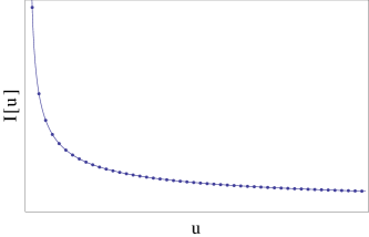
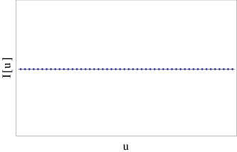
Figure 3: Test of the approximations used in the analytical calculation for scattering with the modes at $\pi$ and $\pi(1\pm 2M)$. The integral $I(u)=\int_{p}\int_{q}\frac{\delta(\xi_{\sigma{\boldsymbol{p}}})\delta(\xi_{\sigma^{\prime}{\boldsymbol{q}}+{\boldsymbol{p}}+Q})}{N_{\sigma}N_{\sigma^{\prime}}}|V(p)|^{2}|V(q+p+Q)|^{2}{\text{Im}\chi^{R}(u,q_{\|}+Q)}$ is numerically evaluated (dots) and the scaling compared to the analytical expression $I(u)\propto u^{1-2\gamma}$ (solid) for $\gamma=3/4$ and $\gamma=1/2$.

In the main text, we have considered the contribution to the self-energy due to scattering with staggered, commensurate ($S_{+}S_{-}$) and incommensurate ($S_{z}S_{z}$) spin modes. The corresponding spin susceptibilities are given by

$\displaystyle{\text{Im}\chi_{\sigma\sigma^{\prime}}^{R}(\nu,q_{\|})}$ =ฯ‡ฯƒโ€‹ฯƒโ€ฒ0โ€‹sinโก(ฮณฯƒโ€‹ฯƒโ€ฒโ€‹ฯ€)โ€‹sgnโ€‹(ฮฝ)โ€‹ฮ˜โ€‹(ฮฝ2โˆ’vs2โ€‹qโˆฅ2)|โˆ’ฮฝ2+vs2โ€‹qโˆฅ2|ฮณฯƒโ€‹ฯƒโ€ฒabsentsuperscriptsubscript๐œ’๐œŽsuperscript๐œŽโ€ฒ0subscript๐›พ๐œŽsuperscript๐œŽโ€ฒ๐œ‹sgn๐œˆฮ˜superscript๐œˆ2superscriptsubscript๐‘ฃ๐‘ 2superscriptsubscript๐‘žโˆฅ2superscriptsuperscript๐œˆ2superscriptsubscript๐‘ฃ๐‘ 2superscriptsubscript๐‘žโˆฅ2subscript๐›พ๐œŽsuperscript๐œŽโ€ฒ\displaystyle=\chi_{\sigma\sigma^{\prime}}^{0}\sin(\gamma_{\sigma\sigma^{\prime}}\pi)\text{sgn}(\nu)\frac{\Theta(\nu^{2}-v_{s}^{2}q_{\|}^{2})}{|-\nu^{2}+v_{s}^{2}q_{\|}^{2}|^{\gamma_{\sigma\sigma^{\prime}}}} (24)

with $\gamma_{\sigma,\bar{\sigma}}=1-1/(4K)$ ($\bar{\sigma}=-\sigma$) and $\gamma_{\sigma,\sigma}=1-K$. To obtain the corresponding frequency dependence of the self-energy, we use the following analytical approximations

$\displaystyle\Gamma_{\sigma\sigma^{\prime}}^{c}(\omega)$ =J2โ€‹ฯ‡+โˆ’c,0โ€‹sinโกฮณโ€‹ฯ€2โ€‹โˆซ๐‘‘uโ€‹(sgnโ€‹(u)โˆ’sgnโ€‹(u+ฯ‰))โ€‹โˆซpโˆซqsgnโ€‹(u)โ€‹ฮ˜โ€‹(u2โˆ’vs2โ€‹qโˆฅ2)|u2โˆ’vs2โ€‹qโˆฅ2|ฮณโ€‹|Vโ€‹(p)|2โ€‹|Vโ€‹(q+p+Q)|2โ€‹ฮดโ€‹(ฮพฯƒโ€‹๐’‘)โ€‹ฮดโ€‹(ฮพฯƒยฏโ€‹๐’‘+๐’’+Q)Nฯƒโ€‹Nฯƒยฏabsentsuperscript๐ฝ2superscriptsubscript๐œ’absent๐‘0๐›พ๐œ‹2differential-d๐‘ขsgn๐‘ขsgn๐‘ข๐œ”subscript๐‘subscript๐‘žsgn๐‘ขฮ˜superscript๐‘ข2superscriptsubscript๐‘ฃ๐‘ 2superscriptsubscript๐‘žโˆฅ2superscriptsuperscript๐‘ข2superscriptsubscript๐‘ฃ๐‘ 2superscriptsubscript๐‘žโˆฅ2๐›พsuperscript๐‘‰๐‘2superscript๐‘‰๐‘ž๐‘๐‘„2๐›ฟsubscript๐œ‰๐œŽ๐’‘๐›ฟsubscript๐œ‰ยฏ๐œŽ๐’‘๐’’๐‘„subscript๐‘๐œŽsubscript๐‘ยฏ๐œŽ\displaystyle=\frac{J^{2}\chi_{+-}^{c,0}\sin\gamma\pi}{2}\int du({\text{sgn}(u)}-{\text{sgn}(u+\omega)})\int_{p}\int_{q}{\text{sgn}(u)}\frac{\Theta(u^{2}-v_{s}^{2}q_{\|}^{2})}{|u^{2}-v_{s}^{2}q_{\|}^{2}|^{\gamma}}|V(p)|^{2}|V(q+p+Q)|^{2}\frac{\delta(\xi_{\sigma{\boldsymbol{p}}})\delta(\xi_{\bar{\sigma}{\boldsymbol{p}}+{\boldsymbol{q}}+Q})}{N_{\sigma}N_{\bar{\sigma}}}
โ‰ˆJ2โ€‹ฯ‡+โˆ’c,0โ€‹sinโกฮณโ€‹ฯ€2โ€‹โˆซ๐‘‘uโ€‹(1โˆ’sgnโ€‹(u)โ€‹sgnโ€‹(u+ฯ‰))โ€‹1|u|2โ€‹ฮณโ€‹โˆซpโˆซqฮ˜โ€‹(u2โˆ’vs2โ€‹qโˆฅ2)โ€‹|Vโ€‹(p)|2โ€‹|Vโ€‹(q+p+Q)|2โ€‹ฮดโ€‹(ฮพฯƒโ€‹๐’‘)โ€‹ฮดโ€‹(ฮพฯƒยฏโ€‹๐’‘+๐’’+Q)Nฯƒโ€‹Nฯƒยฏabsentsuperscript๐ฝ2superscriptsubscript๐œ’absent๐‘0๐›พ๐œ‹2differential-d๐‘ข1sgn๐‘ขsgn๐‘ข๐œ”1superscript๐‘ข2๐›พsubscript๐‘subscript๐‘žฮ˜superscript๐‘ข2superscriptsubscript๐‘ฃ๐‘ 2superscriptsubscript๐‘žโˆฅ2superscript๐‘‰๐‘2superscript๐‘‰๐‘ž๐‘๐‘„2๐›ฟsubscript๐œ‰๐œŽ๐’‘๐›ฟsubscript๐œ‰ยฏ๐œŽ๐’‘๐’’๐‘„subscript๐‘๐œŽsubscript๐‘ยฏ๐œŽ\displaystyle\approx\frac{J^{2}\chi_{+-}^{c,0}\sin\gamma\pi}{2}\int du(1-{\text{sgn}(u)}{\text{sgn}(u+\omega)})\frac{1}{|u|^{2\gamma}}\int_{p}\int_{q}\Theta(u^{2}-v_{s}^{2}q_{\|}^{2})|V(p)|^{2}|V(q+p+Q)|^{2}\frac{\delta(\xi_{\sigma{\boldsymbol{p}}})\delta(\xi_{\bar{\sigma}{\boldsymbol{p}}+{\boldsymbol{q}}+Q})}{N_{\sigma}N_{\bar{\sigma}}}
โ‰ˆJ2โ€‹ฯ‡+โˆ’c,0โ€‹sinโกฮณโ€‹ฯ€2โ€‹โˆซ๐‘‘uโ€‹(1โˆ’sgnโ€‹(u)โ€‹sgnโ€‹(u+ฯ‰))โ€‹2โ€‹|u|vsโ€‹|u|2โ€‹ฮณโ€‹โˆซpโˆซq|Vโ€‹(p)|2โ€‹|Vโ€‹(q+p+Q)|2โ€‹ฮดโ€‹(ฮพฯƒโ€‹๐’‘)โ€‹ฮดโ€‹(ฮพฯƒยฏโ€‹๐’‘+๐’’+Q)Nฯƒโ€‹Nฯƒยฏโ€‹ฮดโ€‹(qโˆฅ)absentsuperscript๐ฝ2superscriptsubscript๐œ’absent๐‘0๐›พ๐œ‹2differential-d๐‘ข1sgn๐‘ขsgn๐‘ข๐œ”2๐‘ขsubscript๐‘ฃ๐‘ superscript๐‘ข2๐›พsubscript๐‘subscript๐‘žsuperscript๐‘‰๐‘2superscript๐‘‰๐‘ž๐‘๐‘„2๐›ฟsubscript๐œ‰๐œŽ๐’‘๐›ฟsubscript๐œ‰ยฏ๐œŽ๐’‘๐’’๐‘„subscript๐‘๐œŽsubscript๐‘ยฏ๐œŽ๐›ฟsubscript๐‘žโˆฅ\displaystyle\approx\frac{J^{2}\chi_{+-}^{c,0}\sin\gamma\pi}{2}\int du(1-{\text{sgn}(u)}{\text{sgn}(u+\omega)})\frac{2|u|}{v_{s}|u|^{2\gamma}}\int_{p}\int_{q}|V(p)|^{2}|V(q+p+Q)|^{2}\frac{\delta(\xi_{\sigma{\boldsymbol{p}}})\delta(\xi_{\bar{\sigma}{\boldsymbol{p}}+{\boldsymbol{q}}+Q})}{N_{\sigma}N_{\bar{\sigma}}}\delta(q_{\|})
โ‰ˆฯ‡+โˆ’c,0โ€‹sinโกฮณโ€‹ฯ€2โ€‹โˆซ๐‘‘uโ€‹(1โˆ’sgnโ€‹(u)โ€‹sgnโ€‹(u+ฯ‰))โ€‹2โ€‹|u|vsโ€‹|u|2โ€‹ฮณโ€‹V2^absentsuperscriptsubscript๐œ’absent๐‘0๐›พ๐œ‹2differential-d๐‘ข1sgn๐‘ขsgn๐‘ข๐œ”2๐‘ขsubscript๐‘ฃ๐‘ superscript๐‘ข2๐›พ^superscript๐‘‰2\displaystyle\approx\frac{\chi_{+-}^{c,0}\sin\gamma\pi}{2}\int du(1-{\text{sgn}(u)}{\text{sgn}(u+\omega)})\frac{2|u|}{v_{s}|u|^{2\gamma}}\widehat{V^{2}}
=ฯ‡+โˆ’c,0โ€‹sinโกฮณโ€‹ฯ€vsโ€‹11โˆ’ฮณโ€‹V2^โ€‹|ฯ‰|2โˆ’2โ€‹ฮณabsentsuperscriptsubscript๐œ’absent๐‘0๐›พ๐œ‹subscript๐‘ฃ๐‘ 11๐›พ^superscript๐‘‰2superscript๐œ”22๐›พ\displaystyle=\frac{\chi_{+-}^{c,0}\sin\gamma\pi}{v_{s}}\frac{1}{1-\gamma}\widehat{V^{2}}|\omega|^{2-2\gamma}
$\displaystyle\propto\left\{\begin{matrix}|\omega|^{\frac{1}{2K}}&\sigma^{\prime}=\sigma\\ |\omega|^{2K}&\sigma^{\prime}=-\sigma\end{matrix}\right.$ (25)

with $\widehat{V^{2}}=J^{2}\int_{p}\int_{q}|V(p)|^{2}|V(q+p+Q)|^{2}\frac{\delta(\xi_{\sigma{\boldsymbol{p}}})\delta(\xi_{\bar{\sigma}{\boldsymbol{p}}+{\boldsymbol{q}}+Q})}{N_{\sigma}N_{\bar{\sigma}}}$. Here, we have discarded terms of higher order in frequency than the leading term $\omega^{2-2\gamma}$ and approximated the prefactor by the average of the squared coupling due to simplicity. To check our approximations, we have calculated, the momentum integral in the first line numerically. The result is shown in Fig.ย 3. Indeed, we obtain the correct scaling with our analytical analysis.

Let us also note that formally, we have to distinguish

ฯ‡ฯƒโ€‹ฯƒsโ€‹(iโ€‹ฯ‰,qโˆฅ)superscriptsubscript๐œ’๐œŽ๐œŽ๐‘ ๐‘–๐œ”subscript๐‘žโˆฅ\displaystyle\chi_{\sigma\sigma}^{s}(i\omega,q_{\|}) $\displaystyle=\chi_{\sigma\sigma}^{s,0}\frac{1}{(\omega^{2}+v_{s}^{2}q_{||}^{2})^{1-K}}\quad\text{if }K<1$ (26)
ฯ‡ฯƒโ€‹ฯƒsโ€‹(iโ€‹ฯ‰,qโˆฅ)superscriptsubscript๐œ’๐œŽ๐œŽ๐‘ ๐‘–๐œ”subscript๐‘žโˆฅ\displaystyle\chi_{\sigma\sigma}^{s}(i\omega,q_{\|}) $\displaystyle=\chi_{\sigma\sigma}^{s,0}\ln\frac{(v_{s}\Lambda)^{2}}{\omega^{2}+v_{s}^{2}q_{||}^{2}}\quad\text{if }K=1,$ (27)

In the case $K\approx 1$ of incommensurate $S_{z}S_{z}$ modes; the imaginary part of the spin susceptibility is then

Imโ€‹ฯ‡ziโ€‹c,Rโ€‹(ฮฝ,q)=ฯ‡ziโ€‹c,0โ€‹ฯ€โ€‹sgnโ€‹(ฮฝ)โ€‹ฮ˜โ€‹(ฮฝ2โˆ’vs2โ€‹q2)Imsuperscriptsubscript๐œ’๐‘ง๐‘–๐‘๐‘…๐œˆ๐‘žsuperscriptsubscript๐œ’๐‘ง๐‘–๐‘0๐œ‹sgn๐œˆฮ˜superscript๐œˆ2superscriptsubscript๐‘ฃ๐‘ 2superscript๐‘ž2{\text{Im}\chi_{z}^{ic,R}(\nu,q)}=\chi_{z}^{ic,0}\pi\text{sgn}(\nu)\Theta(\nu^{2}-v_{s}^{2}q^{2}) (28)

Hence we find for the incommensurate modes around $\pi(1\pm 2M)$

$\displaystyle\Gamma_{\sigma\sigma}^{ic}(\omega)$ โ‰ˆJ2โ€‹ฯ‡ziโ€‹c,0โ€‹ฯ€2โ€‹โˆซ(1โˆ’sgnโ€‹(u)โ€‹sgnโ€‹(u+ฯ‰))โ€‹2โ€‹|u|vsโ€‹โˆซpโˆซq|Vโ€‹(p)|2โ€‹|Vโ€‹(q+p+Q)|2โ€‹ฮดโ€‹(ฮพฯƒโ€‹๐’‘)โ€‹ฮดโ€‹(ฮพฯƒโ€‹๐’‘+๐’’+Q)Nฯƒ2absentsuperscript๐ฝ2superscriptsubscript๐œ’๐‘ง๐‘–๐‘0๐œ‹21sgn๐‘ขsgn๐‘ข๐œ”2๐‘ขsubscript๐‘ฃ๐‘ subscript๐‘subscript๐‘žsuperscript๐‘‰๐‘2superscript๐‘‰๐‘ž๐‘๐‘„2๐›ฟsubscript๐œ‰๐œŽ๐’‘๐›ฟsubscript๐œ‰๐œŽ๐’‘๐’’๐‘„superscriptsubscript๐‘๐œŽ2\displaystyle\approx\frac{J^{2}\chi_{z}^{ic,0}\pi}{2}\int(1-{\text{sgn}(u)}{\text{sgn}(u+\omega)})\frac{2|u|}{v_{s}}\int_{p}\int_{q}|V(p)|^{2}|V(q+p+Q)|^{2}\frac{\delta(\xi_{\sigma{\boldsymbol{p}}})\delta(\xi_{\sigma{\boldsymbol{p}}+{\boldsymbol{q}}+Q})}{N_{\sigma}^{2}}
=J2โ€‹ฯ‡ziโ€‹c,0โ€‹ฯ€vsโ€‹ฯ‰2โ€‹โˆซpโˆซq|Vโ€‹(p)|2โ€‹|Vโ€‹(q+p+Q)|2โ€‹ฮดโ€‹(ฮพฯƒโ€‹๐’‘)โ€‹ฮดโ€‹(ฮพฯƒโ€‹๐’‘+๐’’+Q)Nฯƒ2absentsuperscript๐ฝ2superscriptsubscript๐œ’๐‘ง๐‘–๐‘0๐œ‹subscript๐‘ฃ๐‘ superscript๐œ”2subscript๐‘subscript๐‘žsuperscript๐‘‰๐‘2superscript๐‘‰๐‘ž๐‘๐‘„2๐›ฟsubscript๐œ‰๐œŽ๐’‘๐›ฟsubscript๐œ‰๐œŽ๐’‘๐’’๐‘„superscriptsubscript๐‘๐œŽ2\displaystyle=\frac{J^{2}\chi_{z}^{ic,0}\pi}{v_{s}}\omega^{2}\int_{p}\int_{q}|V(p)|^{2}|V(q+p+Q)|^{2}\frac{\delta(\xi_{\sigma{\boldsymbol{p}}})\delta(\xi_{\sigma{\boldsymbol{p}}+{\boldsymbol{q}}+Q})}{N_{\sigma}^{2}} (29)

which coincides with the limit $K\rightarrow 1$ of the expression for general $K$.

A.4 Relaxation rate from uniform spin correlations

To perform the integrals in the general expression for the electron self-energy, we have to take the different spin susceptibilities into account. Here we present the calculations for the subleading modes, which have been omitted in the main text. We will use the same approximations as for the staggered modes, which we checked numerically above.

For the commensurate $S_{z}S_{z}$ correlations, we have

Imโ€‹ฯ‡zc,Rโ€‹(ฮฝ,q)=ฯ‡zc,0โ€‹ฯ€โ€‹sgnโ€‹(ฮฝ)โ€‹qz2โ€‹ฮดโ€‹(โˆ’ฮฝ2+vs2โ€‹q2)Imsuperscriptsubscript๐œ’๐‘ง๐‘๐‘…๐œˆ๐‘žsuperscriptsubscript๐œ’๐‘ง๐‘0๐œ‹sgn๐œˆsuperscriptsubscript๐‘ž๐‘ง2๐›ฟsuperscript๐œˆ2superscriptsubscript๐‘ฃ๐‘ 2superscript๐‘ž2{\text{Im}\chi_{z}^{c,R}(\nu,q)}=\chi_{z}^{c,0}\pi\text{sgn}(\nu)q_{z}^{2}\delta(-\nu^{2}+v_{s}^{2}q^{2}) (30)

For zero temperature, this leads to

$\displaystyle\Gamma_{\sigma\sigma}^{c}(\omega)$ =J2โ€‹ฯ‡zc,0โ€‹ฯ€2โ€‹โˆซ๐‘‘uโ€‹(sgnโ€‹(u)โˆ’sgnโ€‹(u+ฯ‰))โ€‹โˆซpโˆซqqโˆฅ2โ€‹sgnโ€‹(u)โ€‹ฮดโ€‹(u2โˆ’vs2โ€‹qโˆฅ2)โ€‹(pโˆฅ2+pโŸ‚,12p2)3โ€‹((qโˆฅ+pโˆฅ)2+(qโŸ‚,1+pโŸ‚,1)2(q+p)2)3absentsuperscript๐ฝ2superscriptsubscript๐œ’๐‘ง๐‘0๐œ‹2differential-d๐‘ขsgn๐‘ขsgn๐‘ข๐œ”subscript๐‘subscript๐‘žsuperscriptsubscript๐‘žโˆฅ2sgn๐‘ข๐›ฟsuperscript๐‘ข2superscriptsubscript๐‘ฃ๐‘ 2superscriptsubscript๐‘žโˆฅ2superscriptsuperscriptsubscript๐‘โˆฅ2superscriptsubscript๐‘perpendicular-to12superscript๐‘23superscriptsuperscriptsubscript๐‘žโˆฅsubscript๐‘โˆฅ2superscriptsubscript๐‘žperpendicular-to1subscript๐‘perpendicular-to12superscript๐‘ž๐‘23\displaystyle=\frac{J^{2}\chi_{z}^{c,0}\pi}{2}\int du({\text{sgn}(u)}-{\text{sgn}(u+\omega)})\int_{p}\int_{q}q_{\|}^{2}{\text{sgn}(u)}\delta(u^{2}-v_{s}^{2}q_{\|}^{2})\left(\frac{p_{\|}^{2}+p_{\perp,1}^{2}}{p^{2}}\right)^{3}\left(\frac{(q_{\|}+p_{\|})^{2}+(q_{\perp,1}+p_{\perp,1})^{2}}{(q+p)^{2}}\right)^{3}
$\displaystyle\hskip 184.9429pt\times\frac{\delta(\xi_{\sigma{\boldsymbol{p}}})\delta(\xi_{\sigma{\boldsymbol{p}}+{\boldsymbol{q}}})}{N_{\sigma}^{2}}$
=J2โ€‹ฯ‡zc,0โ€‹ฯ€2โ€‹โˆซ๐‘‘uโ€‹(1โˆ’sgnโ€‹(u)โ€‹sgnโ€‹(u+ฯ‰))โ€‹โˆซpโˆซq|qโˆฅ|2โ€‹vs2โ€‹(ฮดโ€‹(qโˆฅโˆ’uvs)+ฮดโ€‹(qโˆฅ+uvs))โ€‹(pโˆฅ2+pโŸ‚,12p2)3absentsuperscript๐ฝ2superscriptsubscript๐œ’๐‘ง๐‘0๐œ‹2differential-d๐‘ข1sgn๐‘ขsgn๐‘ข๐œ”subscript๐‘subscript๐‘žsubscript๐‘žโˆฅ2superscriptsubscript๐‘ฃ๐‘ 2๐›ฟsubscript๐‘žโˆฅ๐‘ขsubscript๐‘ฃ๐‘ ๐›ฟsubscript๐‘žโˆฅ๐‘ขsubscript๐‘ฃ๐‘ superscriptsuperscriptsubscript๐‘โˆฅ2superscriptsubscript๐‘perpendicular-to12superscript๐‘23\displaystyle=\frac{J^{2}\chi_{z}^{c,0}\pi}{2}\int du(1-{\text{sgn}(u)}{\text{sgn}(u+\omega)})\int_{p}\int_{q}\frac{|q_{\|}|}{2v_{s}^{2}}\left(\delta(q_{\|}-\frac{u}{v_{s}})+\delta(q_{\|}+\frac{u}{v_{s}})\right)\left(\frac{p_{\|}^{2}+p_{\perp,1}^{2}}{p^{2}}\right)^{3}
$\displaystyle\hskip 184.9429pt\times\left(\frac{(q_{\|}+p_{\|})^{2}+(q_{\perp,1}+p_{\perp,1})^{2}}{(q+p)^{2}}\right)^{3}\frac{\delta(\xi_{\sigma{\boldsymbol{p}}})\delta(\xi_{\sigma{\boldsymbol{p}}+{\boldsymbol{q}}})}{N_{\sigma}^{2}}$
=J2โ€‹ฯ‡zc,0โ€‹ฯ€2โ€‹โˆซ0|ฯ‰|๐‘‘uโ€‹2โ€‹|u|2โ€‹vs3โ€‹โˆซpโˆซd2โ€‹qโŸ‚(2โ€‹ฯ€)3โ€‹(pโˆฅ2+pโŸ‚,12p2)3โ€‹ฮดโ€‹(ฮพฯƒโ€‹๐’‘)Nฯƒ2โ€‹[|Vโ€‹(q+p)|2โ€‹ฮดโ€‹(ฮพฯƒโ€‹๐’‘+๐’’)|qโˆฅ=uvs+|Vโ€‹(q+p)|2โ€‹ฮดโ€‹(ฮพฯƒโ€‹๐’‘+๐’’)|qโˆฅ=โˆ’uvs]absentsuperscript๐ฝ2superscriptsubscript๐œ’๐‘ง๐‘0๐œ‹2superscriptsubscript0๐œ”differential-d๐‘ข2๐‘ข2superscriptsubscript๐‘ฃ๐‘ 3subscript๐‘superscript๐‘‘2subscript๐‘žperpendicular-tosuperscript2๐œ‹3superscriptsuperscriptsubscript๐‘โˆฅ2superscriptsubscript๐‘perpendicular-to12superscript๐‘23๐›ฟsubscript๐œ‰๐œŽ๐’‘superscriptsubscript๐‘๐œŽ2delimited-[]evaluated-atsuperscript๐‘‰๐‘ž๐‘2๐›ฟsubscript๐œ‰๐œŽ๐’‘๐’’subscript๐‘žโˆฅ๐‘ขsubscript๐‘ฃ๐‘ evaluated-atsuperscript๐‘‰๐‘ž๐‘2๐›ฟsubscript๐œ‰๐œŽ๐’‘๐’’subscript๐‘žโˆฅ๐‘ขsubscript๐‘ฃ๐‘ \displaystyle=\frac{J^{2}\chi_{z}^{c,0}\pi}{2}\int_{0}^{|\omega|}du2\frac{|u|}{2v_{s}^{3}}\int_{p}\int\frac{d^{2}q_{\perp}}{(2\pi)^{3}}\!\left(\frac{p_{\|}^{2}+p_{\perp,1}^{2}}{p^{2}}\right)^{3}\!\!\frac{\delta(\xi_{\sigma{\boldsymbol{p}}})}{N_{\sigma}^{2}}\!\left[|V(q+p)|^{2}\delta(\xi_{\sigma{\boldsymbol{p}}+{\boldsymbol{q}}})|_{q_{\|}=\frac{u}{v_{s}}}+|V(q+p)|^{2}\delta(\xi_{\sigma{\boldsymbol{p}}+{\boldsymbol{q}}})|_{q_{\|}=-\frac{u}{v_{s}}}\right]
โ‰ˆJ2โ€‹ฯ‡zc,0โ€‹ฯ€2โ€‹vs3โ€‹ฯ‰2โ€‹โˆซpโˆซq|Vโ€‹(p)|2โ€‹|Vโ€‹(q+p)|2โ€‹ฮดโ€‹(ฮพฯƒโ€‹๐’‘)โ€‹ฮดโ€‹(ฮพฯƒโ€‹๐’‘+๐’’)Nฯƒ2absentsuperscript๐ฝ2superscriptsubscript๐œ’๐‘ง๐‘0๐œ‹2superscriptsubscript๐‘ฃ๐‘ 3superscript๐œ”2subscript๐‘subscript๐‘žsuperscript๐‘‰๐‘2superscript๐‘‰๐‘ž๐‘2๐›ฟsubscript๐œ‰๐œŽ๐’‘๐›ฟsubscript๐œ‰๐œŽ๐’‘๐’’superscriptsubscript๐‘๐œŽ2\displaystyle\approx\frac{J^{2}\chi_{z}^{c,0}\pi}{2v_{s}^{3}}\omega^{2}\int_{p}\int_{q}|V(p)|^{2}|V(q+p)|^{2}\frac{\delta(\xi_{\sigma{\boldsymbol{p}}})\delta(\xi_{\sigma{\boldsymbol{p}}+{\boldsymbol{q}}})}{N_{\sigma}^{2}} (31)

Similarly, to lowest order in $\omega$, the FS-averaged relaxation rate due to incommensurate $S_{+}S_{-}$ modes around $\pm 2\pi M$ with

Imโ€‹ฯ‡+โˆ’iโ€‹c,Rโ€‹(ฮฝ,q)=ฯ‡+โˆ’iโ€‹c,0โ€‹sinโก(ฮฒโ€‹ฯ€)โ€‹sgnโ€‹(ฮฝ)โ€‹ฮฝ2+vs2โ€‹qโˆฅ2|โˆ’ฮฝ2+vs2โ€‹q2|ฮฒโ€‹ฮ˜โ€‹(ฮฝ2โˆ’vs2โ€‹q2)ฮฒ=2โˆ’Kโˆ’14โ€‹Kformulae-sequenceImsuperscriptsubscript๐œ’absent๐‘–๐‘๐‘…๐œˆ๐‘žsuperscriptsubscript๐œ’absent๐‘–๐‘0๐›ฝ๐œ‹sgn๐œˆsuperscript๐œˆ2superscriptsubscript๐‘ฃ๐‘ 2superscriptsubscript๐‘žโˆฅ2superscriptsuperscript๐œˆ2superscriptsubscript๐‘ฃ๐‘ 2superscript๐‘ž2๐›ฝฮ˜superscript๐œˆ2superscriptsubscript๐‘ฃ๐‘ 2superscript๐‘ž2๐›ฝ2๐พ14๐พ{\text{Im}\chi_{+-}^{ic,R}(\nu,q)}=\chi_{+-}^{ic,0}\sin(\beta\pi)\text{sgn}(\nu)\frac{\nu^{2}+v_{s}^{2}q_{\|}^{2}}{|-\nu^{2}+v_{s}^{2}q^{2}|^{\beta}}\Theta(\nu^{2}-v_{s}^{2}q^{2})\quad\quad\quad\beta=2-K-\frac{1}{4K} (32)

is

$\displaystyle\Gamma_{\sigma\bar{\sigma}}^{ic}(\omega)$ =J2โ€‹ฯ‡+โˆ’iโ€‹c,0โ€‹sinโกฮฒโ€‹ฯ€2โ€‹โˆซ๐‘‘uโ€‹(sgnโ€‹(u)โˆ’sgnโ€‹(u+ฯ‰))โ€‹โˆซpโˆซqsgnโ€‹(u)โ€‹u2+vs2โ€‹qโˆฅ2|u2โˆ’vs2โ€‹qโˆฅ2|ฮฒโ€‹ฮ˜โ€‹(u2โˆ’vs2โ€‹qโˆฅ2)โ€‹|Vโ€‹(p)|2โ€‹|Vโ€‹(q+p+Q)|2absentsuperscript๐ฝ2superscriptsubscript๐œ’absent๐‘–๐‘0๐›ฝ๐œ‹2differential-d๐‘ขsgn๐‘ขsgn๐‘ข๐œ”subscript๐‘subscript๐‘žsgn๐‘ขsuperscript๐‘ข2superscriptsubscript๐‘ฃ๐‘ 2superscriptsubscript๐‘žโˆฅ2superscriptsuperscript๐‘ข2superscriptsubscript๐‘ฃ๐‘ 2superscriptsubscript๐‘žโˆฅ2๐›ฝฮ˜superscript๐‘ข2superscriptsubscript๐‘ฃ๐‘ 2superscriptsubscript๐‘žโˆฅ2superscript๐‘‰๐‘2superscript๐‘‰๐‘ž๐‘๐‘„2\displaystyle=\frac{J^{2}\chi_{+-}^{ic,0}\sin\beta\pi}{2}\int du({\text{sgn}(u)}-{\text{sgn}(u+\omega)})\int_{p}\int_{q}{\text{sgn}(u)}\frac{u^{2}+v_{s}^{2}q_{\|}^{2}}{|u^{2}-v_{s}^{2}q_{\|}^{2}|^{\beta}}\Theta(u^{2}-v_{s}^{2}q_{\|}^{2})|V(p)|^{2}|V(q+p+Q)|^{2}
$\displaystyle\hskip 199.16928pt\times\frac{\delta(\xi_{\sigma{\boldsymbol{p}}})\delta(\xi_{\bar{\sigma}{\boldsymbol{p}}+{\boldsymbol{q}}+Q})}{N_{\sigma}N_{\bar{\sigma}}}$
โ‰ˆJ2โ€‹ฯ‡+โˆ’iโ€‹c,0โ€‹sinโกฮฒโ€‹ฯ€2โ€‹โˆซ๐‘‘uโ€‹(1โˆ’sgnโ€‹(u)โ€‹sgnโ€‹(u+ฯ‰))โ€‹2โ€‹|u|vsโ€‹u2|u|2โ€‹ฮฒโ€‹โˆซpโˆซq|Vโ€‹(p)|2โ€‹|Vโ€‹(q+p+Q)|2โ€‹ฮดโ€‹(ฮพฯƒโ€‹๐’‘)โ€‹ฮดโ€‹(ฮพฯƒยฏโ€‹๐’‘+๐’’+Q)Nฯƒโ€‹Nฯƒยฏabsentsuperscript๐ฝ2superscriptsubscript๐œ’absent๐‘–๐‘0๐›ฝ๐œ‹2differential-d๐‘ข1sgn๐‘ขsgn๐‘ข๐œ”2๐‘ขsubscript๐‘ฃ๐‘ superscript๐‘ข2superscript๐‘ข2๐›ฝsubscript๐‘subscript๐‘žsuperscript๐‘‰๐‘2superscript๐‘‰๐‘ž๐‘๐‘„2๐›ฟsubscript๐œ‰๐œŽ๐’‘๐›ฟsubscript๐œ‰ยฏ๐œŽ๐’‘๐’’๐‘„subscript๐‘๐œŽsubscript๐‘ยฏ๐œŽ\displaystyle\approx\frac{J^{2}\chi_{+-}^{ic,0}\sin\beta\pi}{2}\int du(1-{\text{sgn}(u)}{\text{sgn}(u+\omega)})\frac{2|u|}{v_{s}}\frac{u^{2}}{|u|^{2\beta}}\int_{p}\int_{q}|V(p)|^{2}|V(q+p+Q)|^{2}\frac{\delta(\xi_{\sigma{\boldsymbol{p}}})\delta(\xi_{\bar{\sigma}{\boldsymbol{p}}+{\boldsymbol{q}}+Q})}{N_{\sigma}N_{\bar{\sigma}}}
=J2โ€‹ฯ‡+โˆ’iโ€‹c,0โ€‹sinโกฮฒโ€‹ฯ€vsโ€‹12โˆ’ฮฒโ€‹|ฯ‰|4โˆ’2โ€‹ฮฒโ€‹โˆซpโˆซq|Vโ€‹(p)|2โ€‹|Vโ€‹(q+p+Q)|2โ€‹ฮดโ€‹(ฮพฯƒโ€‹๐’‘)โ€‹ฮดโ€‹(ฮพฯƒยฏโ€‹๐’‘+๐’’+Q)Nฯƒโ€‹Nฯƒยฏabsentsuperscript๐ฝ2superscriptsubscript๐œ’absent๐‘–๐‘0๐›ฝ๐œ‹subscript๐‘ฃ๐‘ 12๐›ฝsuperscript๐œ”42๐›ฝsubscript๐‘subscript๐‘žsuperscript๐‘‰๐‘2superscript๐‘‰๐‘ž๐‘๐‘„2๐›ฟsubscript๐œ‰๐œŽ๐’‘๐›ฟsubscript๐œ‰ยฏ๐œŽ๐’‘๐’’๐‘„subscript๐‘๐œŽsubscript๐‘ยฏ๐œŽ\displaystyle=\frac{J^{2}\chi_{+-}^{ic,0}\sin\beta\pi}{v_{s}}\frac{1}{2-\beta}|\omega|^{4-2\beta}\int_{p}\int_{q}|V(p)|^{2}|V(q+p+Q)|^{2}\frac{\delta(\xi_{\sigma{\boldsymbol{p}}})\delta(\xi_{\bar{\sigma}{\boldsymbol{p}}+{\boldsymbol{q}}+Q})}{N_{\sigma}N_{\bar{\sigma}}}
$\displaystyle\propto|\omega|^{2K+\frac{1}{2K}}$ (33)

In the Luttinger liquid regime, $K$ varies between $1/4$ and $1$ and for an extended magnetic field regime it is close to $1/2$. Thus, the leading contribution to the full relaxation rate $\Gamma_{\sigma}(\omega)=\sum_{i,\sigma^{\prime}}N_{\sigma^{\prime}}\int du(n_{B}(u)+n_{F}(u+\omega))\Gamma_{\sigma\sigma^{\prime}}^{i}$ comes from $\Gamma_{\sigma\sigma}^{ic}$ and $\Gamma_{\sigma\bar{\sigma}}^{c}$, i.e. the staggered $S_{z}S_{z}$ and $S_{+}S_{-}$ modes around $Q\sim\pi(1\pm 2\pi M)$ and $Q\sim\pi$, respectively. This is why we focus on them in the main text.

A.5 Adding the polarization bubble

When adding the polarization bubble to the bare spin propagator, i.e. ฯ‡โˆ’1โ€‹(ฮฝ,q)=ฯ‡bโ€‹aโ€‹rโ€‹eโˆ’1โ€‹(ฮฝ,q)+ฮ โ€‹(ฮฝ,q)superscript๐œ’1๐œˆ๐‘žsubscriptsuperscript๐œ’1๐‘๐‘Ž๐‘Ÿ๐‘’๐œˆ๐‘žฮ ๐œˆ๐‘ž\chi^{-1}(\nu,q)=\chi^{-1}_{bare}(\nu,q)+\Pi(\nu,q) with ฮ โ€‹(ฮฝ,q)โ‰ˆโˆ’ฮ rโˆ’iโ€‹ฯ„๐’’โŸ‚โ€‹ฮฝฮ ๐œˆ๐‘žsubscriptฮ ๐‘Ÿ๐‘–subscript๐œsubscript๐’’perpendicular-to๐œˆ\Pi(\nu,q)\approx-\Pi_{r}-i\tau_{{\boldsymbol{q}}_{\perp}}\nu, the imaginary part of the spin propagator becomes

$\displaystyle{\text{Im}\chi}^{i,R}_{\sigma\sigma^{\prime}}(\nu,q)=$ ฯ‡ฯƒโ€‹ฯƒโ€ฒi,0โ€‹ฮ˜โ€‹(ฮฝ2โˆ’vs2โ€‹q2)โ€‹ฯ„~๐’’โŸ‚โ€‹ฮฝ+sgnโ€‹(ฮฝ)โ€‹sinโก(ฮณiโ€‹ฯ€)โ€‹|โˆ’ฮฝ2+vs2โ€‹q2|ฮณi(โˆ’ฮ ~r+cosโก(ฮณiโ€‹ฯ€)โ€‹|โˆ’ฮฝ2+vs2โ€‹qq|ฮณi)2+(ฯ„~๐’’โŸ‚โ€‹ฮฝ+sgnโ€‹(ฮฝ)โ€‹sinโก(ฮณiโ€‹ฯ€)โ€‹|โˆ’ฮฝ2+vs2โ€‹qq|ฮณi)2superscriptsubscript๐œ’๐œŽsuperscript๐œŽโ€ฒ๐‘–0ฮ˜superscript๐œˆ2superscriptsubscript๐‘ฃ๐‘ 2superscript๐‘ž2subscript~๐œsubscript๐’’perpendicular-to๐œˆsgn๐œˆsubscript๐›พ๐‘–๐œ‹superscriptsuperscript๐œˆ2superscriptsubscript๐‘ฃ๐‘ 2superscript๐‘ž2subscript๐›พ๐‘–superscriptsubscript~ฮ ๐‘Ÿsubscript๐›พ๐‘–๐œ‹superscriptsuperscript๐œˆ2superscriptsubscript๐‘ฃ๐‘ 2superscript๐‘ž๐‘žsubscript๐›พ๐‘–2superscriptsubscript~๐œsubscript๐’’perpendicular-to๐œˆsgn๐œˆsubscript๐›พ๐‘–๐œ‹superscriptsuperscript๐œˆ2superscriptsubscript๐‘ฃ๐‘ 2superscript๐‘ž๐‘žsubscript๐›พ๐‘–2\displaystyle\chi_{\sigma\sigma^{\prime}}^{i,0}\,\Theta(\nu^{2}-v_{s}^{2}q^{2})\frac{\tilde{\tau}_{{\boldsymbol{q}}_{\perp}}\nu+\text{sgn}(\nu)\sin(\gamma_{i}\pi)|-\nu^{2}+v_{s}^{2}q^{2}|^{\gamma_{i}}}{\Big{(}-\tilde{\Pi}_{r}+\cos(\gamma_{i}\pi)|-\nu^{2}+v_{s}^{2}q^{q}|^{\gamma_{i}}\Big{)}^{2}+\Big{(}\tilde{\tau}_{{\boldsymbol{q}}_{\perp}}\nu+\text{sgn}(\nu)\sin(\gamma_{i}\pi)|-\nu^{2}+v_{s}^{2}q^{q}|^{\gamma_{i}}\Big{)}^{2}}
$\displaystyle+$ ฯ‡ฯƒโ€‹ฯƒโ€ฒi,0โ€‹ฮ˜โ€‹(vs2โ€‹q2โˆ’ฮฝ2)โ€‹ฯ„~๐’’โŸ‚โ€‹ฮฝฯ„~๐’’โŸ‚2โ€‹ฮฝ2+(โˆ’ฮ ~r+|โˆ’ฮฝ2+vs2โ€‹q2|ฮณi)2superscriptsubscript๐œ’๐œŽsuperscript๐œŽโ€ฒ๐‘–0ฮ˜superscriptsubscript๐‘ฃ๐‘ 2superscript๐‘ž2superscript๐œˆ2subscript~๐œsubscript๐’’perpendicular-to๐œˆsuperscriptsubscript~๐œsubscript๐’’perpendicular-to2superscript๐œˆ2superscriptsubscript~ฮ ๐‘Ÿsuperscriptsuperscript๐œˆ2superscriptsubscript๐‘ฃ๐‘ 2superscript๐‘ž2subscript๐›พ๐‘–2\displaystyle\chi_{\sigma\sigma^{\prime}}^{i,0}\,\Theta(v_{s}^{2}q^{2}-\nu^{2})\frac{\tilde{\tau}_{{\boldsymbol{q}}_{\perp}}\nu}{\tilde{\tau}_{{\boldsymbol{q}}_{\perp}}^{2}\nu^{2}+\Big{(}-\tilde{\Pi}_{r}+|-\nu^{2}+v_{s}^{2}q^{2}|^{\gamma_{i}}\Big{)}^{2}} (34)

with $\gamma_{i}=\gamma_{\sigma\sigma},\gamma_{\sigma\bar{\sigma}}$ and $\tilde{\tau}=\chi_{0}\tau$, ฮ ~r=ฯ‡0โ€‹ฮ rsubscript~ฮ ๐‘Ÿsubscript๐œ’0subscriptฮ ๐‘Ÿ\tilde{\Pi}_{r}=\chi_{0}\Pi_{r}. The contribution from small internal frequencies in the lower row induces behavior linear in frequency. For sufficiently small $\tau\nu$, this contribution looks like a Delta distribution and we obtain

$\displaystyle\Gamma_{\sigma\sigma^{\prime}}$ =J2โ€‹ฯ‡ฯƒโ€‹ฯƒโ€ฒi,0โ€‹ฯ€2โ€‹โˆซ๐‘‘uโ€‹(1โˆ’sgnโ€‹(u)โ€‹sgnโ€‹(u+ฯ‰))โ€‹โˆซpโˆซqฮ˜โ€‹(vs2โ€‹qโˆฅ2โˆ’u2)โ€‹ฮดโ€‹(โˆ’ฮ ~r+|u2โˆ’vs2โ€‹qโˆฅ2|ฮณi)โ€‹|Vโ€‹(p)|2โ€‹|Vโ€‹(p+q+Q)|2absentsuperscript๐ฝ2superscriptsubscript๐œ’๐œŽsuperscript๐œŽโ€ฒ๐‘–0๐œ‹2differential-d๐‘ข1sgn๐‘ขsgn๐‘ข๐œ”subscript๐‘subscript๐‘žฮ˜superscriptsubscript๐‘ฃ๐‘ 2superscriptsubscript๐‘žโˆฅ2superscript๐‘ข2๐›ฟsubscript~ฮ ๐‘Ÿsuperscriptsuperscript๐‘ข2superscriptsubscript๐‘ฃ๐‘ 2superscriptsubscript๐‘žโˆฅ2subscript๐›พ๐‘–superscript๐‘‰๐‘2superscript๐‘‰๐‘๐‘ž๐‘„2\displaystyle=\frac{J^{2}\chi_{\sigma\sigma^{\prime}}^{i,0}\pi}{2}\int du(1-{\text{sgn}(u)}{\text{sgn}(u+\omega)})\int_{p}\int_{q}\Theta(v_{s}^{2}q_{\|}^{2}-u^{2})\delta(-\tilde{\Pi}_{r}+|u^{2}-v_{s}^{2}q_{\|}^{2}|^{\gamma_{i}})|V(p)|^{2}|V(p+q+Q)|^{2}
$\displaystyle\hskip 184.9429pt\times\frac{\delta(\xi_{\sigma{\boldsymbol{p}}})\delta(\xi_{\sigma^{\prime}{\boldsymbol{p}}+{\boldsymbol{q}}+Q})}{N_{\sigma}N_{\sigma^{\prime}}}$
=J2โ€‹ฯ‡ฯƒโ€‹ฯƒโ€ฒi,0โ€‹ฯ€2โ€‹โˆซ๐‘‘uโ€‹(1โˆ’sgnโ€‹(u)โ€‹sgnโ€‹(u+ฯ‰))โ€‹โˆซpโˆซqฮ˜โ€‹(vs2โ€‹qโˆฅ2โˆ’u2)โ€‹ฮดโ€‹(qโˆฅ+1vsโ€‹ฮ ~r1/ฮณi+u2)+ฮดโ€‹(qโˆฅโˆ’1vsโ€‹ฮ ~r1/ฮณi+u2)2โ€‹vsโ€‹ฮณiโ€‹ฮ ~r1โˆ’1/ฮณiโ€‹ฮ ~r1/ฮณi+u2absentsuperscript๐ฝ2superscriptsubscript๐œ’๐œŽsuperscript๐œŽโ€ฒ๐‘–0๐œ‹2differential-d๐‘ข1sgn๐‘ขsgn๐‘ข๐œ”subscript๐‘subscript๐‘žฮ˜superscriptsubscript๐‘ฃ๐‘ 2superscriptsubscript๐‘žโˆฅ2superscript๐‘ข2๐›ฟsubscript๐‘žโˆฅ1subscript๐‘ฃ๐‘ superscriptsubscript~ฮ ๐‘Ÿ1subscript๐›พ๐‘–superscript๐‘ข2๐›ฟsubscript๐‘žโˆฅ1subscript๐‘ฃ๐‘ superscriptsubscript~ฮ ๐‘Ÿ1subscript๐›พ๐‘–superscript๐‘ข22subscript๐‘ฃ๐‘ subscript๐›พ๐‘–superscriptsubscript~ฮ ๐‘Ÿ11subscript๐›พ๐‘–superscriptsubscript~ฮ ๐‘Ÿ1subscript๐›พ๐‘–superscript๐‘ข2\displaystyle=\frac{J^{2}\chi_{\sigma\sigma^{\prime}}^{i,0}\pi}{2}\int du(1-{\text{sgn}(u)}{\text{sgn}(u+\omega)})\int_{p}\int_{q}\Theta(v_{s}^{2}q_{\|}^{2}-u^{2})\frac{\delta(q_{\|}+\frac{1}{v_{s}}\sqrt{\tilde{\Pi}_{r}^{1/\gamma_{i}}+u^{2}})+\delta(q_{\|}-\frac{1}{v_{s}}\sqrt{\tilde{\Pi}_{r}^{1/\gamma_{i}}+u^{2}})}{2v_{s}\gamma_{i}\tilde{\Pi}_{r}^{1-1/\gamma_{i}}\sqrt{\tilde{\Pi}_{r}^{1/\gamma_{i}}+u^{2}}}
$\displaystyle\hskip 184.9429pt\times|V(p)|^{2}|V(p+q+Q)|^{2}\frac{\delta(\xi_{\sigma{\boldsymbol{p}}})\delta(\xi_{\sigma^{\prime}{\boldsymbol{p}}+{\boldsymbol{q}}+Q})}{N_{\sigma}N_{\sigma^{\prime}}}$
โ‰ˆJ2โ€‹ฯ‡ฯƒโ€‹ฯƒโ€ฒi,0โ€‹ฯ€2โ€‹โˆซ๐‘‘uโ€‹2โ€‹1โˆ’sgnโ€‹(u)โ€‹sgnโ€‹(u+ฯ‰)2โ€‹vsโ€‹ฮณiโ€‹ฮ ~r1โˆ’1/(2โ€‹ฮณi)โ€‹โˆซpโˆซq|Vโ€‹(p)|2โ€‹|Vโ€‹(p+q+Q)|2โ€‹ฮดโ€‹(ฮพฯƒโ€‹๐’‘)โ€‹ฮดโ€‹(ฮพฯƒโ€ฒโ€‹๐’‘+๐’’+Q)Nฯƒโ€‹Nฯƒโ€ฒabsentsuperscript๐ฝ2superscriptsubscript๐œ’๐œŽsuperscript๐œŽโ€ฒ๐‘–0๐œ‹2differential-d๐‘ข21sgn๐‘ขsgn๐‘ข๐œ”2subscript๐‘ฃ๐‘ subscript๐›พ๐‘–superscriptsubscript~ฮ ๐‘Ÿ112subscript๐›พ๐‘–subscript๐‘subscript๐‘žsuperscript๐‘‰๐‘2superscript๐‘‰๐‘๐‘ž๐‘„2๐›ฟsubscript๐œ‰๐œŽ๐’‘๐›ฟsubscript๐œ‰superscript๐œŽโ€ฒ๐’‘๐’’๐‘„subscript๐‘๐œŽsubscript๐‘superscript๐œŽโ€ฒ\displaystyle\approx\frac{J^{2}\chi_{\sigma\sigma^{\prime}}^{i,0}\pi}{2}\int du2\frac{1-{\text{sgn}(u)}{\text{sgn}(u+\omega)}}{2v_{s}\gamma_{i}\tilde{\Pi}_{r}^{1-1/(2\gamma_{i})}}\int_{p}\int_{q}|V(p)|^{2}|V(p+q+Q)|^{2}\frac{\delta(\xi_{\sigma{\boldsymbol{p}}})\delta(\xi_{\sigma^{\prime}{\boldsymbol{p}}+{\boldsymbol{q}}+Q})}{N_{\sigma}N_{\sigma^{\prime}}}
=J2โ€‹ฯ‡ฯƒโ€‹ฯƒโ€ฒi,0โ€‹ฯ€vsโ€‹ฮณiโ€‹ฮ ~r1โˆ’1/(2โ€‹ฮณi)โ€‹|ฯ‰|โ€‹โˆซpโˆซq|Vโ€‹(p)|2โ€‹|Vโ€‹(p+q+Q)|2โ€‹ฮดโ€‹(ฮพฯƒโ€‹๐’‘)โ€‹ฮดโ€‹(ฮพฯƒโ€ฒโ€‹๐’‘+๐’’+Q)Nฯƒโ€‹Nฯƒโ€ฒabsentsuperscript๐ฝ2superscriptsubscript๐œ’๐œŽsuperscript๐œŽโ€ฒ๐‘–0๐œ‹subscript๐‘ฃ๐‘ subscript๐›พ๐‘–superscriptsubscript~ฮ ๐‘Ÿ112subscript๐›พ๐‘–๐œ”subscript๐‘subscript๐‘žsuperscript๐‘‰๐‘2superscript๐‘‰๐‘๐‘ž๐‘„2๐›ฟsubscript๐œ‰๐œŽ๐’‘๐›ฟsubscript๐œ‰superscript๐œŽโ€ฒ๐’‘๐’’๐‘„subscript๐‘๐œŽsubscript๐‘superscript๐œŽโ€ฒ\displaystyle=\frac{J^{2}\chi_{\sigma\sigma^{\prime}}^{i,0}\pi}{v_{s}\gamma_{i}\tilde{\Pi}_{r}^{1-1/(2\gamma_{i})}}|\omega|\int_{p}\int_{q}|V(p)|^{2}|V(p+q+Q)|^{2}\frac{\delta(\xi_{\sigma{\boldsymbol{p}}})\delta(\xi_{\sigma^{\prime}{\boldsymbol{p}}+{\boldsymbol{q}}+Q})}{N_{\sigma}N_{\sigma^{\prime}}} (35)

We see that the result scales linearly in frequency.

A.6 Conductivity

A.6.1 General Form

The conductivity is given by the retarded current-current correlation function (we are interested in the diagonal compontents)

$\displaystyle\sigma_{a}(\omega,{\boldsymbol{q}})$ =iฯ‰โ€‹ฮ jaRโ€‹(ฯ‰,๐’’),absent๐‘–๐œ”subscriptsuperscriptฮ ๐‘…subscript๐‘—๐‘Ž๐œ”๐’’\displaystyle=\frac{i}{\omega}\Pi^{R}_{j_{a}}(\omega,{\boldsymbol{q}}), (36)
ฮ jaโ€‹(iโ€‹ฯ‰,๐’’)subscriptฮ subscript๐‘—๐‘Ž๐‘–๐œ”๐’’\displaystyle\Pi_{j_{a}}(i\omega,{\boldsymbol{q}}) $\displaystyle=-\frac{1}{V}\int_{0}^{\beta}d\tau e^{i\omega\tau}\langle T_{\tau}j_{a}(\tau,{\boldsymbol{q}})j_{a}(0,{\boldsymbol{q}})\rangle$ (37)

with volume $V$, time ordering $T_{\tau}$ and $a$-component of the current operator ${\boldsymbol{j}}$. The dc conductivity is obtained by taking the limits $q\rightarrow 0$, and then $\omega\rightarrow 0$ of the expression with the retarded current correlation function (order of limits is important). In our case, we have to distinguish the current for spin up and down ${\boldsymbol{j}}={\boldsymbol{j}}_{\uparrow}+{\boldsymbol{j}}_{\downarrow}$, so that we consider ฯƒ=ฯƒโ†‘+ฯƒโ†“=iฯ‰โ€‹[ฮ j,โ†‘Rโ€‹(ฯ‰,๐’’)+ฮ j,โ†“Rโ€‹(ฯ‰,๐’’)]๐œŽsubscript๐œŽโ†‘subscript๐œŽโ†“๐‘–๐œ”delimited-[]subscriptsuperscriptฮ ๐‘…๐‘—โ†‘๐œ”๐’’subscriptsuperscriptฮ ๐‘…๐‘—โ†“๐œ”๐’’\sigma=\sigma_{\uparrow}+\sigma_{\downarrow}=\frac{i}{\omega}\left[\Pi^{R}_{j,\uparrow}(\omega,{\boldsymbol{q}})+\Pi^{R}_{j,\downarrow}(\omega,{\boldsymbol{q}})\right]. Let us define the current vertex ${\boldsymbol{\Gamma}}_{a}^{\sigma}=p_{a}\gamma_{\sigma}$. Then the static current-current correlation function becomes

$\displaystyle\pi_{a}^{\sigma}(i\omega)$ =limqโ†’0ฮ ja,ฯƒโ€‹(iโ€‹ฯ‰,๐’’)absentsubscriptโ†’๐‘ž0subscriptฮ subscript๐‘—๐‘Ž๐œŽ๐‘–๐œ”๐’’\displaystyle=\lim_{q\rightarrow 0}\Pi_{j_{a},\sigma}(i\omega,{\boldsymbol{q}})
$\displaystyle=\frac{2e^{2}}{m^{2}}\int\frac{d^{3}p}{(2\pi)^{3}}T\sum_{ip}G_{\sigma}(ip,{\boldsymbol{p}})G_{\sigma}(ip+i\omega,{\boldsymbol{p}})p_{a}\Gamma_{a}^{\sigma}({\boldsymbol{p}},ip,ip+i\omega)$
$\displaystyle=\frac{2e^{2}}{m^{2}}\int\frac{d^{3}p}{(2\pi)^{3}}p_{a}^{2}T\sum_{ip}G_{\sigma}(ip,{\boldsymbol{p}})G_{\sigma}(ip+i\omega,{\boldsymbol{p}})\gamma_{\sigma}({\boldsymbol{p}},ip,ip+i\omega)$ (38)

In our case, we want to distinguish directions parallel and perpendicular to the chains, i.e. we consider

$\displaystyle\pi_{\|}^{\sigma}(i\omega)$ $\displaystyle=\frac{2e^{2}}{m^{2}}\int\frac{d^{3}p}{(2\pi)^{3}}p_{\|}^{2}T\sum_{ip}G_{\sigma}(ip,{\boldsymbol{p}})G_{\sigma}(ip+i\omega,{\boldsymbol{p}})\gamma_{\sigma}({\boldsymbol{p}},ip,ip+i\omega)$ (39)
$\displaystyle\pi_{\perp}^{\sigma}(i\omega)$ $\displaystyle=\frac{e^{2}}{m^{2}}\int\frac{d^{3}p}{(2\pi)^{3}}{\boldsymbol{p}}_{\perp}^{2}T\sum_{ip}G_{\sigma}(ip,{\boldsymbol{p}})G_{\sigma}(ip+i\omega,{\boldsymbol{p}})\gamma_{\sigma}({\boldsymbol{p}},ip,ip+i\omega),$ (40)

where the factor of $1/2$ is added because both perpendicular directions yield the same result so that $\pi^{\sigma}_{\perp}=\pi^{\sigma}_{x}=\pi^{\sigma}_{y}$.

After evaluating the Matsubara summation, the dc conductivity becomes (Ref. Mahan Ch. 8.4.2)

$\displaystyle\sigma_{\|/\perp}^{\sigma}=$ $\displaystyle\frac{1}{1+\delta_{\perp,\|/\perp}}\frac{e^{2}}{m^{2}}\int\frac{d^{3}p}{(2\pi)^{2}}p_{\|/\perp}^{2}\int\frac{d\epsilon}{2\pi}\left(-\frac{dn_{F}}{d\epsilon}\right)$
$\displaystyle\times\left[G_{\sigma}({\boldsymbol{p}},\epsilon+i\delta)G_{\sigma}({\boldsymbol{p}},\epsilon-i\delta)\gamma_{\sigma}({\boldsymbol{p}},\epsilon-i\delta,\epsilon+i\delta)+\text{Re}\Big{(}G^{2}_{\sigma}({\boldsymbol{p}},\epsilon+i\delta)\gamma_{\sigma}({\boldsymbol{p}},\epsilon+i\delta,\epsilon+i\delta)\Big{)}\right]$ (41)

The second term in the brackets will vanish by doing the integration over $\xi=p^{2}/(2m)-\mu$, which is why we will not consider it in the following. Furthermore, we use that due to the Greenโ€™s functions, the dominant contribution comes from momenta close to the FS and that we are only interested in scaling with frequency or temperature, i.e. we can replace $|G_{\sigma}|^{2}\approx\delta(\xi_{\sigma{\boldsymbol{p}}})/\Gamma(\epsilon)$. This leads to

$\displaystyle\sigma^{\sigma}_{i}$ $\displaystyle\approx\frac{2e^{2}}{c_{i}m^{2}}\int\frac{d\epsilon}{2\pi}\left(-\frac{dn_{F}}{d\epsilon}\right)\int_{p}p_{i}^{2}\frac{\delta(\xi_{\sigma{\boldsymbol{p}}})}{\Gamma_{\sigma}(\epsilon)}\gamma_{\sigma}({\boldsymbol{p}},\epsilon)$
$\displaystyle=\frac{2e^{2}}{c_{i}m^{2}}\int\frac{d\epsilon}{2\pi}\left(-\frac{dn_{F}}{d\epsilon}\right)\frac{1}{\Gamma_{\sigma}(\epsilon)}p_{F\sigma}^{2}\int_{p}\frac{p_{i}^{2}}{p^{2}}\delta(\xi_{\sigma{\boldsymbol{p}}})\gamma_{\sigma}({\boldsymbol{p}},\epsilon)$
$\displaystyle=\frac{6e^{2}n_{\sigma}}{c_{i}m}\int\frac{d\epsilon}{2\pi}\left(-\frac{dn_{F}}{d\epsilon}\right)\frac{1}{\Gamma_{\sigma}(\epsilon)}\frac{1}{N_{\sigma}}\int_{p}\frac{p_{i}^{2}}{p^{2}}\delta(\xi_{\sigma{\boldsymbol{p}}})\gamma_{\sigma}({\boldsymbol{p}},\epsilon)$
$\displaystyle=:\frac{6e^{2}n_{\sigma}}{c_{i}m}\int\frac{d\epsilon}{2\pi}\left(-\frac{dn_{F}}{d\epsilon}\right)\frac{\gamma^{i}_{\sigma}(\epsilon)}{\Gamma_{\sigma}(\epsilon)}$ (42)

with $c_{i}=1+\delta_{i\perp}$, $\gamma_{\sigma}({\boldsymbol{p}},\epsilon)=\gamma_{\sigma}({\boldsymbol{p}},\epsilon-i\delta,\epsilon+i\delta)$, density of states $N_{\sigma}=p_{F\sigma}m/(2\pi^{2})$ and number density $n_{\sigma}=p_{F\sigma}^{3}/(6\pi^{2})$. We have defined the FS-averaged, scalar current vertex $\gamma^{i}_{\sigma}(\epsilon)=\frac{1}{N_{\sigma}}\int_{p}\frac{p_{i}^{2}}{p^{2}}\delta(\xi_{\sigma{\boldsymbol{p}}})\gamma_{\sigma}({\boldsymbol{p}},\epsilon)$. We observe that

$$\gamma_{\sigma}(\epsilon)=\frac{1}{N_{\sigma}}\int_{p}\delta(\xi_{\sigma{\boldsymbol{p}}})\gamma_{\sigma}({\boldsymbol{p}},\epsilon)=\frac{1}{N_{\sigma}}\int_{p}\frac{p_{\|}^{2}+{\boldsymbol{p}}_{\perp}^{2}}{p^{2}}\delta(\xi_{\sigma{\boldsymbol{p}}})\gamma_{\sigma}({\boldsymbol{p}},\epsilon)=\gamma^{\|}_{\sigma}(\epsilon)+\gamma^{\perp}_{\sigma}(\epsilon)$$ (43)

A.6.2 Vertex function

To obtain the scalar vertex functions $\gamma_{\sigma}^{\perp/\|}$, we sum the ladder diagrams for the current vertex. This leads to the Dyson equation for the vertex of the form

$\displaystyle{\boldsymbol{p}}\gamma_{\sigma}({\boldsymbol{p}},ip,ip+i\omega)=$ $\displaystyle{\boldsymbol{p}}+J^{2}\sum_{\sigma^{\prime}}T\sum_{iq}\int_{q}|V(p)|^{2}|V(q)|^{2}\chi_{\sigma\sigma^{\prime}}(iq-ip,{\boldsymbol{q}}-{\boldsymbol{p}})G(iq,{\boldsymbol{q}})G(iq+i\omega,{\boldsymbol{q}}){\boldsymbol{q}}\gamma_{\sigma^{\prime}}({\boldsymbol{q}},iq,iq+i\omega).$ (44)

After performing the Matsubara summation and again approximating $|G_{\sigma}|^{2}\approx\frac{\delta(\xi_{{\boldsymbol{p}}\sigma})}{\Gamma_{\sigma}(\epsilon)}$, the equation for $\gamma_{\sigma}({\boldsymbol{p}},\epsilon-i\delta,\epsilon+i\delta)$ becomes

$\displaystyle{\boldsymbol{p}}\gamma_{\sigma}({\boldsymbol{p}},\epsilon)=$ $\displaystyle{\boldsymbol{p}}+J^{2}\sum_{\sigma^{\prime}}\int dx\int_{q}|V(p)|^{2}|V(q)|^{2}{\text{Im}\chi}^{R}_{\sigma\sigma^{\prime}}(x,{\boldsymbol{q}}-{\boldsymbol{p}})\left[n_{B}(x)+n_{F}(\epsilon+x)\right]\frac{\delta(\xi_{{\boldsymbol{q}}\sigma^{\prime}})}{\Gamma_{\sigma^{\prime}}(\epsilon+x)}{\boldsymbol{q}}\gamma_{\sigma^{\prime}}({\boldsymbol{q}},\epsilon+x).$ (45)

Thus the averages over the Fermi surface satisfy

$\displaystyle\gamma_{\sigma}^{i}(\epsilon)$ $\displaystyle=\int_{p}\frac{\delta(\xi_{{\boldsymbol{p}}\sigma})}{N_{\sigma}}\frac{p_{i}^{2}}{p^{2}}\gamma_{\sigma}({\boldsymbol{p}},\epsilon)$
$\displaystyle=m_{i}+J^{2}\sum_{\sigma^{\prime}}N_{\sigma^{\prime}}\int dx\int_{p}\int_{q}|V(p)|^{2}|V(q)|^{2}{\text{Im}\chi}^{R}_{\sigma\sigma^{\prime}}(x,{\boldsymbol{q}}-{\boldsymbol{p}})\left[n_{B}(x)+n_{F}(\epsilon+x)\right]\frac{\delta(\xi_{{\boldsymbol{p}}\sigma})\delta(\xi_{{\boldsymbol{q}}\sigma^{\prime}})}{N_{\sigma}N_{\sigma^{\prime}}}\frac{{\boldsymbol{p}}_{i}{\boldsymbol{q}}_{i}}{p^{2}}\frac{\gamma_{\sigma^{\prime}}({\boldsymbol{q}},\epsilon+x)}{\Gamma_{\sigma^{\prime}}(\epsilon+x)}.$ (46)

with

$$m_{i}=\int_{p}\frac{\delta(\xi_{{\boldsymbol{p}}\sigma})}{N_{\sigma}}\frac{p_{i}^{2}}{p^{2}}$$ (47)

and

$\displaystyle\gamma_{\sigma}(\epsilon)$ $\displaystyle=\int_{p}\frac{\delta(\xi_{{\boldsymbol{p}}\sigma})}{N_{\sigma}}\gamma_{\sigma}({\boldsymbol{p}},\epsilon)$
$\displaystyle=1+J^{2}\sum_{\sigma^{\prime}}N_{\sigma^{\prime}}\int dx\int_{p}\int_{q}|V(p)|^{2}|V(q)|^{2}{\text{Im}\chi}^{R}_{\sigma\sigma^{\prime}}(x,{\boldsymbol{q}}-{\boldsymbol{p}})\left[n_{B}(x)+n_{F}(\epsilon+x)\right]\frac{\delta(\xi_{{\boldsymbol{p}}\sigma})\delta(\xi_{{\boldsymbol{q}}\sigma^{\prime}})}{N_{\sigma}N_{\sigma^{\prime}}}\frac{{\boldsymbol{p}}{\boldsymbol{q}}}{p^{2}}\frac{\gamma_{\sigma^{\prime}}({\boldsymbol{q}},\epsilon+x)}{\Gamma_{\sigma^{\prime}}(\epsilon+x)}$
$\displaystyle=1+J^{2}\sum_{\sigma^{\prime}}N_{\sigma^{\prime}}\int dx\int_{p}\int_{q}|V(p)|^{2}|V(q)|^{2}{\text{Im}\chi}^{R}_{\sigma\sigma^{\prime}}(x,{\boldsymbol{q}}-{\boldsymbol{p}})\left[n_{B}(x)+n_{F}(\epsilon+x)\right]\frac{\delta(\xi_{{\boldsymbol{p}}\sigma})\delta(\xi_{{\boldsymbol{q}}\sigma^{\prime}})}{N_{\sigma}N_{\sigma^{\prime}}}\frac{{\boldsymbol{p}}{\boldsymbol{q}}}{p^{2}}$
$\displaystyle\hskip 85.35826pt\times\frac{1}{\Gamma_{\sigma^{\prime}}(\epsilon+x)}\int dx\int_{q}\frac{\delta(\xi_{{\boldsymbol{q}}\sigma^{\prime}})}{N_{\sigma^{\prime}}}\gamma_{\sigma^{\prime}}({\boldsymbol{q}},\epsilon+x)$
$\displaystyle=1+\sum_{\sigma^{\prime}}N_{\sigma^{\prime}}\int du[n_{B}(u)+n_{F}(u+\epsilon)]I_{\sigma\sigma^{\prime}}(u)\frac{\gamma_{\sigma^{\prime}}(\epsilon+u)}{\Gamma_{\sigma^{\prime}}(\epsilon+u)}.$ (48)

In the last line we have defined $I_{\sigma\sigma^{\prime}}(u)=J^{2}\int_{p}\int_{q}|V(p)|^{2}|V(q)|^{2}{\text{Im}\chi}^{R}_{\sigma\sigma^{\prime}}(u,{\boldsymbol{q}}-{\boldsymbol{p}})\frac{\delta(\xi_{{\boldsymbol{p}}\sigma})\delta(\xi_{{\boldsymbol{q}}\sigma^{\prime}})}{N_{\sigma}N_{\sigma^{\prime}}}\frac{{\boldsymbol{p}}{\boldsymbol{q}}}{p^{2}}$. The integral $I_{\sigma\sigma^{\prime}}$ can be rewritten as a sum of relaxation rate and a transport rate

$\displaystyle I_{\sigma\sigma^{\prime}}=J^{2}\int_{p}\int_{q}|V({\boldsymbol{p}})|^{2}|V({\boldsymbol{q}}+{\boldsymbol{p}}+Q_{\sigma\sigma^{\prime}})|^{2}{\text{Im}\chi}^{R}_{\sigma\sigma^{\prime}}(u,{\boldsymbol{q}}+Q_{\sigma\sigma^{\prime}})\frac{\delta(\xi_{{\boldsymbol{p}}\sigma})\delta(\xi_{{\boldsymbol{q}}+{\boldsymbol{p}}+Q\sigma^{\prime}})}{N_{\sigma}N_{\sigma^{\prime}}}\frac{{\boldsymbol{p}}({\boldsymbol{q}}+{\boldsymbol{p}}+Q_{\sigma\sigma^{\prime}})}{p^{2}}$ (49)

with $Q_{\sigma\sigma}=\pi(1\pm 2\pi M)$ and $Q_{\sigma\bar{\sigma}}=\pi$. The product $(p-(q+p+Q))^{2}=p_{F\sigma}^{2}+p_{F\sigma^{\prime}}^{2}-2p(q+p+Q)=(Q+q)^{2}=Q^{2}+2Qq+q^{2}$, so that

$\displaystyle I_{\sigma\sigma^{\prime}}$ $\displaystyle=J^{2}\int_{p}\int_{q}|V({\boldsymbol{p}})|^{2}|V({\boldsymbol{q}}+{\boldsymbol{p}}+Q_{\sigma\sigma^{\prime}})|^{2}{\text{Im}\chi}^{R}_{\sigma\sigma^{\prime}}(u,{\boldsymbol{q}}+Q_{\sigma\sigma^{\prime}})\frac{\delta(\xi_{{\boldsymbol{p}}\sigma})\delta(\xi_{{\boldsymbol{q}}+{\boldsymbol{p}}+Q\sigma^{\prime}})}{N_{\sigma}N_{\sigma^{\prime}}}$
$\displaystyle\hskip 142.26378pt\times\left(\frac{p_{F\sigma}^{2}+p_{F\sigma^{\prime}}^{2}-Q_{\sigma\sigma^{\prime}}^{2}}{2p_{F\sigma}^{2}}-\frac{q(2Q_{\sigma\sigma^{\prime}}+q)}{2p_{F\sigma}^{2}}\right)$
$\displaystyle=f_{\sigma\sigma^{\prime}}\Gamma_{\sigma\sigma^{\prime}}-\Gamma_{\sigma\sigma^{\prime}}^{t}$ (50)

with $f_{\sigma\sigma^{\prime}}=\frac{p_{F\sigma}^{2}+p_{F\sigma^{\prime}}^{2}-Q_{\sigma\sigma^{\prime}}^{2}}{2p_{F\sigma}^{2}}\approx 1-Q^{2}/(2p_{F}^{2})+\mathcal{O}(h/E_{F})$ and $\Gamma_{\sigma\sigma^{\prime}}^{t}=J^{2}\int_{p}\int_{q}|V({\boldsymbol{p}})|^{2}|V({\boldsymbol{q}}+{\boldsymbol{p}}+Q)|^{2}{\text{Im}\chi}^{R}_{\sigma\sigma^{\prime}}(u,{\boldsymbol{q}}+Q)\frac{\delta(\xi_{{\boldsymbol{p}}\sigma})\delta(\xi_{{\boldsymbol{q}}+{\boldsymbol{p}}+Q\sigma^{\prime}})}{N_{\sigma}N_{\sigma^{\prime}}}\frac{q(2Q+q)}{2p_{F\sigma}^{2}}$. To solve the equation for the current vertex $\gamma_{\sigma}(\epsilon)$, we approximate $\frac{\gamma_{\sigma^{\prime}}(\epsilon+x)}{\Gamma_{\sigma^{\prime}}(\epsilon+x)}\rightarrow\frac{\gamma_{\sigma^{\prime}}(\epsilon)}{\Gamma_{\sigma^{\prime}}(\epsilon)}$, which has been shown to lead to the correct low-energy scaling belitz2010 . Due to the additional factor in the transport relaxation rate $\Gamma_{\sigma\sigma^{\prime}}^{t}$, the leading frequency dependence comes from $I_{\sigma\sigma^{\prime}}\approx f_{\sigma\sigma^{\prime}}\Gamma_{\sigma\sigma^{\prime}}$. With this, the scalar current vertex is given by

$\displaystyle\gamma_{\sigma}$ $\displaystyle=\Gamma\frac{\Gamma+f_{\sigma\bar{\sigma}}\Gamma_{+-}-f_{\bar{\sigma}\bar{\sigma}}\Gamma_{z}}{\Gamma^{2}-f_{\sigma\bar{\sigma}}f_{\bar{\sigma}\sigma}\Gamma_{+-}^{2}-(f_{\sigma\sigma}+f_{\bar{\sigma}\bar{\sigma}})\Gamma\Gamma_{z}+f_{\sigma\sigma}f_{\bar{\sigma}\bar{\sigma}}\Gamma_{z}^{2}}$
$\displaystyle\approx\frac{1}{1-f}+\mathcal{O}(h/E_{F}),$ (51)

where we have neglected terms of order of the magnetic field over the Fermi energy $h/E_{F}\ll 1$ and $f=1-Q^{2}/(2p_{F}^{2})$. We cited this result in the main text. Note that this is only the leading contribution for a finite $Q$: if $Q\approx 0$ and $f\rightarrow 1$, this contribution vanishes and the leading behavior is of the form $\gamma_{\sigma}=\Gamma_{\sigma}/\Gamma^{t}_{\sigma}$ with $\Gamma^{t}_{\sigma}=\sum_{\sigma^{\prime}}N_{\sigma^{\prime}}\int du[n_{B}(u)+n_{F}(u+\epsilon)]\Gamma^{t}_{\sigma\sigma^{\prime}}(u)$.

References

  • (1) โ€Concentrated Kondo systemsโ€, N.B. Brandt, V.V. Moshchalkov, Adv. in Phys. 33, 373 (1984).
  • (2) โ€Theories of heavy-electron systemsโ€, P.A. Lee, T.M. Rice, J.W. Serene, L.J. Sham, J.W. Wilkins, Comments on Condensed Matter Physics 12, 99 (1986).
  • (3) โ€Non-Fermi-liquid behavior in $d$- and $f$-electron metalsโ€, G.R. Stewart, Rev. Mod. Phys. 73, 797 (2001).
  • (4) โ€Quantum criticality in heavy-fermion metalsโ€, P. Gegenwart, Q. Si, F. Steglich, Nature Physics 4, 186 (2008).
  • (5) โ€Exploring heavy fermions from macroscopic to microscopic length scalesโ€, S. Wirth and F. Steglich, Nature Reviews Materials 1, 16051 (2016).
  • (6) โ€Heavy-fermion systemsโ€, G.R. Stewart, Rev. Mod. Phys. 56, 755 (1984).
  • (7) โ€The Kondo lattice and weak antiferromagnetismโ€, S. Doniach, Physica B+C 91, 231 (1977).
  • (8) โ€Frustration and the Kondo Effect in Heavy Fermion Materialsโ€, P. Coleman and A.H. Nevidomskyy, J. Low. Temp. Phys. 161, 182 (2010).
  • (9) โ€Structure and Properties of YbZnSn, YbAgSn, and Yb2Pt2Pbโ€, R. Pรถttgen, P.E. Arpe, C. Felser, D. KuรŸmann, R. Mรผllmann, B.D. Mosel, B. Kรผnnen and G. Kotzyba, J. Solid State Chem. 145, 668 (1999).
  • (10) โ€Yb2Pt2Pb: Magnetic frustration in the Shastry-Sutherland latticeโ€, M.S. Kim, M.C. Bennett, and M.C. Aronson, Phys. Rev. B 77, 144425 (2008).
  • (11) โ€Field-Induced Partially Disordered State in Yb2Pt2Pbโ€, A. Ochiai, S. Matsuda, Y. Ikeda, Y. Shimizu, S. Toyoshima, H. Aoki, and K. Katoh, J. Phys. Soc. Jpn. 80, 123705 (2011).
  • (12) โ€Orbital Exchange and Fractional Quantum Number Excitations in an f-electron Metal Yb2Pt2Pbโ€, L. S. Wu, W. J. Gannon, I. A. Zaliznyak, A. M. Tsvelik, M. Brockmann, J.-S. Caux, M.-S. Kim, Y. Qiu, J. R. D. Copley, G. Ehlers, A. Podlesnyak, M. C. Aronson, Science 352, 1206-1210 (2016).
  • (13) โ€Magnetic structure of Yb2Pt2Pb: Ising moments on the Shastry-Sutherland latticeโ€, W. Miiller, L. S. Wu, M. S. Kim, T. Orvis, J. W. Simonson, M. Gamลผa, D. M. McNally, C. S. Nelson, G. Ehlers, A. Podlesnyak, J. S. Helton, Y. Zhao, Y. Qiu, J. R. D. Copley, J. W. Lynn, I. Zaliznyak, and M. C. Aronson, Phys. Rev. B 93, 104419 (2016)
  • (14) โ€Spin Liquids and Antiferromagnetic Order in the Shastry-Sutherland-Lattice Compound Yb2Pt2Pbโ€, M.S. Kim, M.C. Aronson, Phys. Rev. Lett. 110, 017201 (2013).
  • (15) L. S. Wu, PhD thesis, SUNY (2013); L. S. Wu et. al., unpublished.
  • (16) In fact, in Yb2Pt2Pb, there are two kinds of magnetic chains and depending on the direction of the magnetic field either both or only one sublattice undergoes the transition into the Luttinger liquid phase.
  • (17) โ€Field-induced incommensurate order for the quasi-one-dimensional XXZ model in a magnetic fieldโ€, K. Okunishi, T. Suzuki, Phys. Rev. B 76, 224411 (2007).
  • (18) โ€Critical properties of gapped spin-1/2 chains and ladders in a magnetic fieldโ€, R. Chitra and T. Giamarchi, Phys. Rev. B 55, 5816 (1997).
  • (19) โ€Quantum Physics in One Dimensionโ€, T. Giamarchi, Oxford University Press (2003).
  • (20) โ€Quantum Field Theory in Condensed Matter Physicsโ€, A. M. Tsvelik, Cambridge: Cambridge University Press, (2003).
  • (21) โ€Quantum Magnetismโ€, U. Schollwรถck, J. Richter, D.J.J. Farnell, R.F. Bishop (Eds.), Quantum Magnetism, Lect. Notes Phys. 645 (Springer, Berlin Heidelberg 2004).
  • (22) see e.g. โ€œMethods of Quantum Field Theory in Statistical Physicsโ€, A.A. Abrikosov, L.P. Gorkov and I.E. Dzyaloshinski, Dover Publication (1975).
  • (23) see e.g. โ€Many-Particle Physicsโ€, G.D. Mahan, Kluwer Academic/Plenum Publishers, New York (2000).
  • (24) โ€Electronic relaxation rates in metallic ferromagnetsโ€, S. Bharadwaj, D. Belitz, T.R. Kirkpatrick, Phys. Rev. B 89, 134401 (2014).
  • (25) โ€Electronic transport at low temperatures: Diagrammatic approachโ€, D. Belitz, T.R. Kirkpatrick, Physica E 42, 497 (2010).