Robust and scalable methods for the dynamic mode decomposition

Abstract

The dynamic mode decomposition (DMD) is a broadly applicable dimensionality reduction algorithm that approximates a matrix containing time-series data by the outer product of a matrix of exponentials, representing Fourier-like time dynamics, and a matrix of coefficients, representing spatial structures. This interpretable spatio-temporal decomposition is commonly computed using linear algebraic techniques in its simplest formulation or a nonlinear optimization procedure within the variable projection framework. For data with sparse outliers or data which are not well-represented by exponentials in time, the standard Frobenius norm fit of the data creates significant biases in the recovered time dynamics. As a result, practitioners are left to clean such defects from the data manually or to use a black-box cleaning approach like robust PCA. As an alternative, we propose a framework and a set of algorithms for incorporating robust features into the nonlinear optimization used to compute the DMD itself. The algorithms presented are flexible, allowing for regularizers and constraints on the optimization, and scalable, using a stochastic approach to decrease the computational cost for data in high dimensional space. Both synthetic and real data examples are provided.

Keywords: robust statistics, dynamic mode decomposition, scalable algorithms

1 Introduction

Dimensionality reduction is a critically enabling tool in machine learning applications. Specifically, extracting the dominant low-rank features from a high-dimensional data matrix ${\mathbf{X}}\in{\mathbb{R}}^{m\times n}$ allows one to efficiently perform tasks associated with clustering, classification and prediction. As defined by Cunningham and Ghahramani (2015), linear dimensionality reduction methods solve an optimization problem with objective $f_{{\mathbf{X}}}(\cdot)$ over a manifold ${\mathcal{M}}$ to produce a linear transformation $P$ which maps the columns of ${\mathbf{X}}$ to a lower dimensional space. Many popular methods can be written in this framework by an appropriate definition of $f_{{\mathbf{X}}}(\cdot)$ and specification of the manifold $\mathcal{M}$. For instance, the principal component analysis (PCA) may be written as

$$\hat{M}=\operatorname*{argmin}_{M\in\mathcal{M}}\|{\mathbf{X}}-MM^{\intercal}{\mathbf{X}}\|_{F}\,,\qquad\mathcal{M}=\mathcal{O}^{m\times k}\;,$$ (1)

where $\mathcal{O}^{m\times k}$ is the manifold of $m\times k$ matrices with orthonormal columns, i.e. $\mathcal{M}$ is a Stiefel manifold. The map $P$ is then given by $\hat{M}^{\intercal}$. One of the primary conclusions of the survey (Cunningham and Ghahramani, 2015), is that — aside from the PCA itself — many of the common methods for linear dimensionality reduction based on eigenvalue solvers are actually sub-optimal heuristics and the direct solution of the optimization problem (1) should be preferred.

In this manuscript, we consider a particular linear dimensionality reduction technique: the dynamic mode decomposition (DMD). In the past decade, the DMD has been applied to the analysis of fluid flow experiments and simulations, machine learning enabled control systems, and Koopman spectral analysis, among other data-intensive problems described by dynamical systems. The success of the algorithm is largely due to the interpretability of the low-rank spatio-temporal modes it generates in approximating the dominant features of the data matrix ${\bf X}$. The DMD was originally defined to be the output of an algorithm for characterizing time-series measurements of fluid flow data (Schmid and Sesterhenn, 2008; Schmid, 2010). It was later reformulated by Tu et al. (2014) as a least-squares regression problem whereby the DMD could be stably computed using a Moore-Penrose pseudo-inverse and an eigenvalue decomposition. An earlier though less commonly used formulation, the optimized DMD (Chen et al., 2012), can be phrased as the optimization problem

$$\hat{M}=\operatorname*{argmin}_{M\in\mathcal{M}}\|{\mathbf{X}}-MM^{\dagger}{\mathbf{X}}\|_{F}\;,\quad\mathcal{M}={\boldsymbol{\Phi}}({\mathbb{C}}^{k})\;,$$ (2)

where the map ${\boldsymbol{\alpha}}\mapsto{\bf\Phi}({\boldsymbol{\alpha}})$ defines a matrix with columns corresponding to exponential time dynamics (see Section 2.1) and $M^{\dagger}$ denotes the Moore-Penrose pseudo-inverse of $M$. This can be thought of as a best-fit linear dynamical system approximation of the data. In agreement with the conclusions of Cunningham and Ghahramani (2015), the optimized DMD, while more costly to compute, is more robust to additive noise than the exact DMD and its noise-corrected alternatives (Dawson et al., 2016; Askham and Kutz, 2017). It is also more flexible than the exact DMD, allowing for non-equispaced snapshots. While the optimized DMD does not fit directly into the optimization framework of Cunningham and Ghahramani (2015), which is defined for $\mathcal{M}$ either a Stiefel manifold or a Grassmannian manifold, it can be computed efficiently using classical variable projection methods (Golub and LeVeque, 1979; Askham and Kutz, 2017).

The DMD has been used in a variety of fields where the nature of the data can lead to corrupt and noisy measurements. This includes applications ranging from neuroscience (Brunton et al., 2016) to video processing (Grosek and Kutz, 2014; Erichson et al., 2015) to fluid dynamics (Schmid and Sesterhenn, 2008; Schmid, 2010; Guéniat et al., 2015; Dawson et al., 2016). Although the Frobenius norm used in the definition of the optimized DMD (2) is appealing due to its physical interpretability in many applications (energy, mass, etc.), it has significant flaws that can severely limit its applicability. Specifically, corrupt data or large noise fluctuations can lead to significant deformation of the DMD approximation of the data because the Frobenius norm implicitly assigns a very low probability to such outliers (see Section 2.2). In practice, these outliers are often removed from the data manually or using a black-box filtering approach like robust PCA (Locantore et al., 1999; Wright et al., 2009; Candès et al., 2011). However, such approaches ignore the structure of the DMD approximation and may introduce biases of their own. Further, it is desirable that DMD methods not only be robust to “noisy” outliers but also to non-exponential structure in the data. We therefore develop an alternative approach to increase the robustness of the DMD. In particular, we modify the optimized DMD definition (2) to incorporate ideas from the field of robust statistics (Maronna et al., 2006; Huber, 2011) in order to produce a decomposition that is significantly less sensitive to outliers in the data.

Because the new problem formulation incorporates robust norms, many of the efficient strategies used in variable projection algorithms for problems defined in the Frobenius norm are no longer available. To remedy this, we develop a number of algorithms based on modern variable projection methods (Aravkin and Van Leeuwen, 2012; Aravkin et al., 2017) which exploit the structure of the DMD for increased performance. In particular, we can incorporate nonsmooth features, such as regularizers and constraints, and scale to large problems using stochastic variance reduction techniques.

This flexible architecture allows us to impose physically relevant constraints on the optimization that are critical for tasks such as future-state prediction. For instance, we can impose the constraint that the real parts of the DMD eigenvalues are non-positive, thus ensuring that solutions do not grow to infinity when forecasting.

The effect of noise on the DMD is a well-studied area. Controlling for the bias of the exact DMD in the presence of additive noise was treated by Hemati et al. (2017) and Dawson et al. (2016). A Bayesian formulation of the DMD was presented by Takeishi et al. (2017). This formulation is flexible enough to incorporate robust statistics but this was not a focus of that work. Dicle et al. (2016) presented a robust formulation of exact DMD type, which complements the current work.

The rest of this manuscript is organized as follows. In Section 2, we provide some necessary preliminaries from the DMD, robust statistics, and variable projection literature and we present our problem formulation. A detailed description of the algorithms we use to solve the robust DMD formulation follows in Section 3. We apply these methods to synthetic data in Section 4 and to real data in Section 5. Finally, we provide some concluding remarks and describe possible future directions in Section 6.

2 Preliminaries

In this section, we outline some of the precursors of this work and present our problem formulation.

2.1 Dynamic mode decomposition

As mentioned above, the dynamic mode decomposition (DMD) corresponds to a best-fit linear dynamical model of the data. Because linear dynamics produce exponential functions in time, the DMD may be written as an exponential fitting problem. Let ${\mathbf{X}}\in{\mathbb{C}}^{m\times n}$ be a snapshot matrix whose rows ${\mathbf{x}}_{j}$ are samples of an $n$ dimensional dynamical system at a set of $m$ sample times $t_{j}$. For a given rank $k$, let ${\boldsymbol{\alpha}}\in{\mathbb{C}}^{k}$ be a vector of complex numbers specifying time dynamics. We then define the matrix ${\boldsymbol{\Phi}}({\boldsymbol{\alpha}};{\mathbf{t}})$ by

$$\Phi_{ij}({\boldsymbol{\alpha}})=e^{\alpha_{j}t_{i}}\;.$$ (3)

When it is clear in context, we often drop the dependence of ${\boldsymbol{\Phi}}$ on ${\boldsymbol{\alpha}}$ and ${\mathbf{t}}$.

Let ${\mathbf{B}}\in{\mathbb{C}}^{k\times n}$ be a matrix of coefficients for the exponential fit. The so-called optimized DMD (see Chen et al., 2012) is defined to be the solution of the following optimization problem:

$$\min_{{\boldsymbol{\alpha}},{\mathbf{B}}}\dfrac{1}{2}\|{\mathbf{X}}-{\boldsymbol{\Phi}}({\boldsymbol{\alpha}}){\mathbf{B}}\|_{F}^{2}\;.$$ (4)

The problem (4) is a large, nonlinear least squares problem; in particular it is highly non-convex. The classical variable projection framework provides an efficient method for computing a (local) solution.

Let

$$f_{\mbox{opt}}({\boldsymbol{\alpha}},{\mathbf{B}})=\dfrac{1}{2}\|{\mathbf{X}}-{\boldsymbol{\Phi}}({\boldsymbol{\alpha}}){\mathbf{B}}\|_{F}^{2}\;.$$

The classical variable projection framework is based on the observation that for a fixed ${\boldsymbol{\alpha}}$, it is easy to optimize $f_{\mbox{opt}}$ in ${\mathbf{B}}$. In fact, for the least squares case, we have a closed form expression

$${\mathbf{B}}({\boldsymbol{\alpha}}):=\arg\min_{{\mathbf{B}}}f_{\mbox{opt}}({\boldsymbol{\alpha}},{\mathbf{B}})={\boldsymbol{\Phi}}({\boldsymbol{\alpha}})^{\dagger}{\mathbf{X}},$$ (5)

where ${\boldsymbol{\Phi}}({\boldsymbol{\alpha}})^{\dagger}$ denotes the Moore-Penrose pseudo-inverse of ${\boldsymbol{\Phi}}({\boldsymbol{\alpha}})$. Let

$$\tilde{f}_{\mbox{opt}}({\boldsymbol{\alpha}})=\min_{{\mathbf{B}}}f_{\mbox{opt}}({\boldsymbol{\alpha}},{\mathbf{B}}):=\dfrac{1}{2}\|{\mathbf{X}}-{\boldsymbol{\Phi}}({\boldsymbol{\alpha}}){\mathbf{B}}({\boldsymbol{\alpha}})\|_{F}^{2}.$$

The variable projection (VP) technique finds the minimizer of $\tilde{f}_{\mbox{opt}}({\boldsymbol{\alpha}})$ using an iterative method. First and second derivatives of $\tilde{f}$ with respect to ${\boldsymbol{\alpha}}$ are easily computed (see Theorem 2 of Bell and Burke, 2008):

$$\nabla_{{\boldsymbol{\alpha}}}\tilde{f}_{\mbox{opt}}({\boldsymbol{\alpha}}) =\partial_{{\boldsymbol{\alpha}}}f_{\mbox{opt}}|_{{\boldsymbol{\alpha}},{\mathbf{B}}({\boldsymbol{\alpha}})}$$ (6)

$$\nabla_{{\boldsymbol{\alpha}}}^{2}\tilde{f}_{\mbox{opt}}({\boldsymbol{\alpha}}) =\left.\left[\partial^{2}_{{\boldsymbol{\alpha}}}f_{\mbox{opt}}-\partial_{{\boldsymbol{\alpha}},{\mathbf{B}}}f_{\mbox{opt}}(\partial^{2}_{{\mathbf{B}}}f_{\mbox{opt}})^{-1}\partial_{{\mathbf{B}},{\boldsymbol{\alpha}}}f_{\mbox{opt}}\right]\right|_{{\boldsymbol{\alpha}},{\mathbf{B}}({\boldsymbol{\alpha}})}.$$

These formulas allow first- and second-order methods to be directly applied to $\tilde{f}_{\mbox{opt}}$, including steepest descent, BFGS, and Newton’s method. The matrix ${\mathbf{B}}({\boldsymbol{\alpha}})$ is updated every time ${\boldsymbol{\alpha}}$ changes. Gauss-Newton and Levenberg-Marquardt (LM) have been classically used for exponential fitting; these methods do not use the Hessian in (6), opting for simpler approximations. The method was used for exponential fitting by Golub and LeVeque (1979). While VP originally referred to least-squares projection (using the closed-form solution ${\mathbf{B}}({\boldsymbol{\alpha}})$ in (5)), follow-up work considered more general loss functions, using the term projection to refer to partial minimization (Aravkin and Van Leeuwen, 2012; Aravkin et al., 2017).

For practitioners, the optimized DMD may be less familiar than exact DMD (Tu et al., 2014). We favor the optimized DMD for its performance on data with additive noise (see Askham and Kutz, 2017) and its flexibility. In particular, the optimized formulation enables the contributions of the current work. For a review of the DMD and its applications, see Tu et al. (2014) and Kutz et al. (2016).

2.2 Robust Formulations

Figure 1: Gaussian (black dash) and Huber (red solid) Densities, Negative Log Likelihoods, and Influence Functions.

The optimized DMD problem (4) is formulated using the least-squares error norm, which is equivalent to assuming a Gaussian model on the errors between predicted and observed data:

$${\mathbf{X}}={\boldsymbol{\Phi}}({\boldsymbol{\alpha}}){\mathbf{B}}+{\boldsymbol{\epsilon}},\quad{\boldsymbol{\epsilon}}\sim N(0,\sigma^{2}I).$$

This error model, and the corresponding formulation, are vulnerable to outliers in the data. Both DMD and optimized DMD are known to be sensitive to outliers, so in practice data are ‘pre-cleaned’ before applying these approaches.

In many domains, formulations based on robust statics have become the method of choice for dealing with contaminated data. Two common approaches are

• to replace the LS penalty with one that penalizes deviations less harshly and

• to solve an extended problem that explicitly identifies outliers while fitting the model.

The first approach, often called M-estimation (Huber, 2011; Maronna et al., 2006), is illustrated in Figure 1. Replacing the least squares penalty by the Huber penalty

$$\rho(z)=\begin{cases}\frac{1}{2}|z|^{2}&\mbox{if}\;|z|\leq\kappa\\ \kappa|z|-\frac{1}{2}\kappa^{2}&\mbox{if}\;|r|>\kappa\end{cases}$$

corresponds to choosing the solid red penalty rather than the dotted black least squares penalty in the center panel of Figure 1. This corresponds to modeling errors ${\boldsymbol{\epsilon}}$ using the density $\exp(-\rho)$, which has heavier tails than the Gaussian (see left panel of Figure 1). Heavier tails means deviations (i.e. larger residuals) are more likely than under the Gaussian model, and so observations that deviate from the norm have less influence, i.e. effect on the fitted parameters $({\boldsymbol{\alpha}},{\mathbf{B}})$ than under the Gaussian model (see right panel of Figure 1). The M-estimator-DMD problem can be written as

$$\min_{{\boldsymbol{\alpha}},{\mathbf{B}}}\sum_{j=1}^{n}\rho(X_{\cdot j}-{\boldsymbol{\Phi}}({\boldsymbol{\alpha}}){\mathbf{B}}_{j}):=\sum_{j=1}^{n}\rho_{j}({\boldsymbol{\alpha}},{\mathbf{B}}),$$

where the sum is run across columns.

Another approach, called trimmed estimation, builds on M-estimation by coupling explicit outlier identification/removal with model fitting. The trimmed DMD formulation for any penalty $\rho$ is given by

$$\min_{{\boldsymbol{\alpha}},{\mathbf{B}}}\sum_{l=1}^{h}\rho_{j_{l}}({\boldsymbol{\alpha}},{\mathbf{B}}),$$ (7)

where $\rho_{j_{1}}({\boldsymbol{\alpha}},{\mathbf{B}})\leq\cdots\leq\rho_{j_{h}}({\boldsymbol{\alpha}},{\mathbf{B}})$ are the first $h$ order statistics of the objective values and $\{j_{1},\ldots,j_{h}\}\subseteq\{1,\ldots,n\}$. Interpreting the loss $\rho_{j}$ as the negative log likelihood of the $j$th observed column, it is clear that trimming jointly fits a likelihood model while simultaneously eliminating the influence of all low-likelihood observations. An equivalent formulation to (7) replaces the order statistics with explicit weights

$$\min_{{\boldsymbol{\alpha}},{\mathbf{B}},{\mathbf{w}}}\sum_{j=1}^{n}w_{j}\rho_{j}({\boldsymbol{\alpha}},{\mathbf{B}}),\quad 0\leq w_{j}\leq 1,\quad{\mathbf{1}}^{\intercal}{\mathbf{w}}=h.$$ (8)

The reader should verify that (8) and (7) are equivalent.

Trimmed M-estimators were initially introduced by Rousseeuw (1985) in the context of least-squares regression. The author’s original motivation was to develop linear regression estimators that have a high breakdown point (in this case 50%) and good statistical efficiency (in this case $n^{-1/2}$). For a number of years, the difficulty of efficiently optimizing LTS problems limited their application. However, recent work has made it possible to efficiently apply trimming to general models (Yang et al., 2016; Aravkin and Davis, 2016). We show how to incorporate trimming into the robust DMD framework.

2.3 Regularization

Optimized DMD allows prior knowledge to be incorporated into the optimization formulation, either through constraints on variables, or regularization terms. In all exponential fitting problems, the real parts of ${\boldsymbol{\alpha}}$ coefficients play a major role in explaining the data because of the exponential growth of ${\boldsymbol{\Phi}}({\boldsymbol{\alpha}})$. A natural regularization is to restrict the magnitudes of the real parts of ${\boldsymbol{\alpha}}$, imposing the constraint $\mbox{real}({\boldsymbol{\alpha}})\leq\gamma$ with $\gamma$ chosen by the user. We write the constraint as follows:

$$r({\boldsymbol{\alpha}})=\begin{cases}0&\mbox{if}\;\mbox{real}({\boldsymbol{\alpha}})\leq\gamma\\ \infty&\mbox{if}\;\mbox{real}({\boldsymbol{\alpha}})>\gamma.\end{cases}$$

This is a simple convex function that admits a trivial proximal operator (see Combettes and Pesquet (2011)): the projection onto the shifted left half-plane in $\mathbb{C}^{k}$. The VP technique can be easily adapted to incorporate such functions on ${\boldsymbol{\alpha}}$.

Constraints and penalties can also be imposed on the matrix ${\mathbf{B}}$. We assume that only smooth separable regularization penalties can be used; and in this case, the regularization is added to the $g$ function.

2.4 Problem formulation

Let $h({\mathbf{B}})$ and $r({\boldsymbol{\alpha}})$ be convex regularization terms. We formulate the general robust DMD problem as follows:

$$\min_{{\boldsymbol{\alpha}},{\mathbf{B}},{\mathbf{w}}}f({\boldsymbol{\alpha}},{\mathbf{B}},{\mathbf{w}}):=g({\boldsymbol{\alpha}},{\mathbf{B}},{\mathbf{w}})+r({\boldsymbol{\alpha}})+s({\mathbf{w}})\;,$$ (9)

where $r({\boldsymbol{\alpha}})$ encodes optional regularization functions (or constraints) for ${\boldsymbol{\alpha}}$ (see Section 2.3) and

$$g({\boldsymbol{\alpha}},{\mathbf{B}},{\mathbf{w}})=\sum_{j=1}^{n}w_{j}\rho\left(X_{\cdot j}-{\boldsymbol{\Phi}}({\boldsymbol{\alpha}}){\mathbf{B}}_{\cdot j}\right)+q({\mathbf{B}}_{\cdot j})$$ (10)

with $\rho$ any differentiable penalty, $q({\mathbf{B}}_{\cdot j})$ representing potential regularizer for columns of ${\mathbf{B}}$, and $s({\mathbf{w}})$ encoding the capped simplex constraints:

$$s({\mathbf{w}})=\begin{cases}0&\mbox{if}\;0\leq w_{j}\leq 1,\;{\mathbf{1}}^{\intercal}{\mathbf{w}}=h\\ \infty&\mbox{else}.\end{cases}$$ (11)

These constraints are explained in Section 2.2. The ${\mathbf{w}}$ variables select the best-fit $h$ columns of the data, and only use those values to update ${\boldsymbol{\alpha}}$. Since each $w_{j}\in[0,1]$ rather than {0,1}, the solutions do not have to be integral. However, for any fixed $({\mathbf{B}},{\boldsymbol{\alpha}})$ there exists a vertex solution, since the subproblem in ${\mathbf{w}}$ with the other variables fixed is a linear program. The function $s({\mathbf{w}})$ admits a simple proximal operator, which is the projection onto the intersection of the $h$-simplex with the unit cube.

Setting $h=n$ forces $w_{j}=1$ for each column, eliminating trimming completely, and reducing (9) to a simpler regularized M-estimation form of DMD.

For notational convenience, we define a matrix-valued penalty function

$${\boldsymbol{\rho}}(A):=\begin{bmatrix}\rho(A_{1,1})&\cdots&\rho(A_{1,n})\\ \vdots&\ddots&\vdots\\ \rho(A_{m,1})&\cdots&\rho(A_{m,n})\end{bmatrix}.$$

In this notation, we can write

$$g({\boldsymbol{\alpha}},{\mathbf{B}},{\mathbf{w}})={\mathbf{1}}^{\intercal}{\boldsymbol{\rho}}({\mathbf{X}}-{\boldsymbol{\Phi}}({\boldsymbol{\alpha}}){\mathbf{B}}){\mathbf{w}}+q({\mathbf{B}}),$$

which makes derivative computations straightforward.

Our numerical examples use constraints for ${\boldsymbol{\alpha}}$, but do not regularize ${\mathbf{B}}$, that is, $q({\mathbf{B}})\equiv 0$. However, we consider separable penalties $q$ in the algorithmic description to preserve the generality of (9).

2.5 Gradient computations

We need to compute the gradient of the penalty function (10) with respect to the entries of ${\boldsymbol{\alpha}}$ and ${\mathbf{B}}$. In all methods, we treat treat the real and imaginary components of $\alpha_{j}$ and $B_{ji}$ as independent, real-valued parameters.

Consider a complex number $z=x+{\mathbf{i}}y$. We write derivative formulas in the Wirtinger sense, computing partial derivatives with respect to the complex variables. The derivatives for the real components can then be recovered from the formulas

$$\dfrac{\partial}{\partial z}=\dfrac{1}{2}\left(\dfrac{\partial}{\partial x}-{\mathbf{i}}\dfrac{\partial}{\partial y}\right).$$ (12)

Let $g(z)$ be a function of $z$ which can be written as $g(z)=G(z,\bar{z})$ where $G$ is differentiable with respect to both $z$ and $\bar{z}$. The Wirtinger derivative of $g$ is then the partial derivative of $G$ with respect to $z$, treating $\bar{z}$ as a constant. For example, the Huber penalty may be written as

$$\rho(z)=H(z,\bar{z};\kappa)=\begin{cases}\kappa\sqrt{z\bar{z}}-\frac{1}{2}\kappa^{2},&|z|\geq\kappa\\ \frac{1}{2}z\bar{z},&|z|<\kappa\end{cases}\;.$$

The Wirtinger derivative of the Huber penalty is then

$$\rho^{\prime}(z)=\dfrac{\partial}{\partial z}H(z,\bar{z};\kappa)=\begin{cases}\dfrac{\kappa\bar{z}}{2\sqrt{z\bar{z}}},&|z|<\kappa\\ \frac{1}{2}\bar{z},&|z|\geq\kappa\end{cases}\;.$$

The gradients of $f$ with respect to ${\boldsymbol{\alpha}}$ and ${\mathbf{B}}$ can then be computed using the chain rule:

$$\nabla_{\boldsymbol{\alpha}}g({\boldsymbol{\alpha}},{\mathbf{B}},{\mathbf{w}}) =-\operatorname{diag}\left[{\mathbf{B}}\operatorname{Diag}({\mathbf{w}}){\boldsymbol{\rho}}^{\prime}({\mathbf{X}}-{\boldsymbol{\Phi}}{\mathbf{B}})^{\intercal}(\operatorname{Diag}({\mathbf{t}}){\boldsymbol{\Phi}})\right]$$ (13)

$$\nabla_{\mathbf{B}}g({\boldsymbol{\alpha}},{\mathbf{B}},{\mathbf{w}}) =-{\boldsymbol{\Phi}}^{\intercal}{\boldsymbol{\rho}}^{\prime}({\mathbf{X}}-{\boldsymbol{\Phi}}{\mathbf{B}})\operatorname{Diag}({\mathbf{w}})+{\mathbf{B}}^{\intercal}\nabla q({\mathbf{B}})$$

$$\nabla_{\mathbf{w}}g({\boldsymbol{\alpha}},{\mathbf{B}},{\mathbf{w}}) ={\boldsymbol{\rho}}({\mathbf{X}}-{\boldsymbol{\Phi}}{\mathbf{B}})^{\intercal}{\mathbf{1}},$$

where we define

$$\text{diag}(A) :=\begin{bmatrix}a_{11}\\ \vdots\\ \vdots\\ a_{nn}\end{bmatrix},\qquad\text{Diag}(a):=\begin{bmatrix}a_{1}&0&\dots&0\\ 0&a_{2}&\ddots&\vdots\\ \vdots&\ddots&\ddots&0\\ 0&\cdots&0&a_{n}\end{bmatrix}.$$

3 Methods

In this section, we develop numerical approaches for (9).

3.1 Variable projection framework

To compute the robust optimized DMD, we apply the variable projection (VP) technique to the optimization problem (9). Define the reduced function $\tilde{f}$ and implicit solution ${\mathbf{B}}({\boldsymbol{\alpha}})$ by

$$\tilde{f}({\boldsymbol{\alpha}},{\mathbf{w}}) =\min_{\mathbf{B}}f({\boldsymbol{\alpha}},{\mathbf{B}},{\mathbf{w}})\;,$$ (14)

$${\mathbf{B}}({\boldsymbol{\alpha}},{\mathbf{w}}) =\operatorname*{argmin}_{\mathbf{B}}f({\boldsymbol{\alpha}},{\mathbf{B}},{\mathbf{w}})\;,$$

where $f$ is as defined in (9). The gradient formula (6) holds for a very broad problem class. In particular, it holds as long as the following conditions are satisfied (Rockafellar and Wets, 2009, Theorem 10.58):

1. $g({\boldsymbol{\alpha}},{\mathbf{B}},{\mathbf{w}})$ is level-bounded in ${\mathbf{B}}$ locally uniformly in ${\boldsymbol{\alpha}}$; in particular for any compact subset of ${\boldsymbol{\alpha}}$, the union of sublevel sets $\{{\mathbf{B}}:g({\boldsymbol{\alpha}},{\mathbf{B}},{\mathbf{w}})\leq\gamma\}$ is bounded.

2. The gradient of $g({\boldsymbol{\alpha}},{\mathbf{B}},{\mathbf{w}})$ exists and is continuous for all $({\boldsymbol{\alpha}},{\mathbf{B}},{\mathbf{w}})$.

3. ${\mathbf{B}}({\boldsymbol{\alpha}},{\mathbf{w}})$ is unique.

Several assumptions on $g$, ${\boldsymbol{\Phi}}$, and $q$ can be made to ensure these conditions hold. For example, if $g$ is differentiable, convex, coercive in ${\mathbf{B}}$, and ${\boldsymbol{\Phi}}({\boldsymbol{\alpha}})$ has full rank, then the result holds. If the same conditions hold for $g$, ${\boldsymbol{\Phi}}({\boldsymbol{\alpha}})$ does not have full rank, but $q$ is strictly convex, the result holds as well. The derivative formulas are valid for all of the examples in the paper, and we have

$$\nabla\tilde{f}({\boldsymbol{\alpha}},{\mathbf{w}})=\partial_{{\boldsymbol{\alpha}},{\mathbf{w}}}f({\boldsymbol{\alpha}},{\mathbf{B}},{\mathbf{w}})|_{{\boldsymbol{\alpha}},{\mathbf{B}}({\boldsymbol{\alpha}}),{\mathbf{w}}}\;.$$ (15)

We refer to partially minimizing over $f$ over ${\mathbf{B}}$ as the inner problem and minimizing $\tilde{f}$ as the outer problem. When $f$ is convex and smooth with respect to ${\mathbf{B}}$, a lot of fast optimization algorithms can be applied to the inner problem. The inner problem is also embarrassingly parallelizable, and we make use of the problem structure in algorithm design. The general VP strategy is to use an iterative method to compute a (local) minimizer of the reduced function (14).

Solving (9) requires optimization procedures for both the inner and outer problems. We discuss these algorithms in the next two subsections.

3.2 Batch methods

Consider the problem class where $g$ in (9) is convex and continuously differentiable with respect to ${\mathbf{B}}$. In this case, the inner problem decouples into $n$ independent subproblems:

$$_{j}({\boldsymbol{\alpha}},{\mathbf{w}})=\operatorname*{argmin}_{\quad}w_{j}\rho\left(X_{\cdot j}-{\boldsymbol{\Phi}}({\boldsymbol{\alpha}})\right)+q(),\quad j=1,\ldots,n.$$ (16)

We use BFGS to solve each of these subproblems, since the dimension of each problem is relatively small, and BFGS gives a superlinear convergence rate while using only gradient information. When $r$ in (9) is continuously differentiable, we can also use BFGS as our solver, see Algorithm 1. When $r$ is non-smooth but admits an efficient prox operator, a first order method such as the proximal gradient method or its accelerations, such as FISTA (Beck and Teboulle, 2009), can be used instead, see Algorithm 2. We let $\nu$ denote the iteration counter.

Algorithm 1 VP using BFGS for outer problem (smooth $r$).

1:${\boldsymbol{\alpha}}^{0}$, ${\mathbf{B}}^{0}$, ${\mathbf{w}}^{0}$, $H_{\boldsymbol{\alpha}}^{0}=I$, $\nu=0$.

2:while not converged do

3:     for $j=1,\ldots,n$ do

4:         ${}^{\nu+1}_{j}$ $\leftarrow$ $\displaystyle\arg\min_{w}{}_{j}^{\nu}\rho\left(X_{\cdot j}-{\boldsymbol{\Phi}}({\boldsymbol{\alpha}}^{\nu})\right)+q()$      

5:     ${\mathbf{w}}^{\nu+1}$ $\leftarrow$ weights update

6:     $f_{\boldsymbol{\alpha}}^{\nu}$ $\leftarrow$ $f({\boldsymbol{\alpha}}^{\nu},{\mathbf{B}}^{\nu+1},{\mathbf{w}}^{\nu+1})$

7:     $g_{\boldsymbol{\alpha}}^{\nu}$ $\leftarrow$ $\nabla_{\boldsymbol{\alpha}}f({\boldsymbol{\alpha}}^{\nu},{\mathbf{B}}^{\nu+1},{\mathbf{w}}^{\nu+1})$

8:     if $\nu\geq 1$ then

9:         $s^{\nu}$ $\leftarrow$ $f_{\boldsymbol{\alpha}}^{\nu}-f_{\boldsymbol{\alpha}}^{\nu-1}$

10:         $y^{\nu}$ $\leftarrow$ $g_{\boldsymbol{\alpha}}^{\nu}-g_{\boldsymbol{\alpha}}^{\nu-1}$

11:         $\beta^{\nu}$ $\leftarrow$ $(\left\langle s^{\nu},y^{\nu}\right\rangle)^{-1}$

12:         $H_{\boldsymbol{\alpha}}^{\nu}$ $\leftarrow$ $\left[I-\beta^{\nu}(s^{\nu})(y^{\nu})^{\intercal}\right]H^{\nu-1}\left[I-\beta^{\nu}(y^{\nu})(s^{\nu})^{\intercal}\right]+\beta(s^{\nu})(s^{\nu})^{\intercal}$      

13:     ${\boldsymbol{\alpha}}^{\nu+1}$ $\leftarrow$ LineSearch$\left({\boldsymbol{\alpha}}^{\nu}-\eta_{\boldsymbol{\alpha}}H_{\boldsymbol{\alpha}}^{\nu}g_{\boldsymbol{\alpha}}^{\nu}\right)$

14:     $\nu$ $\leftarrow$ $\nu+1$

15:${\boldsymbol{\alpha}}^{\nu}$, ${\mathbf{B}}^{\nu}$.

Algorithm 2 VP using prox-gradient for outer problem (prox-friendly $r$).

1:${\boldsymbol{\alpha}}^{0}$, ${\mathbf{B}}^{0}$, ${\mathbf{w}}^{0}$, $\nu=0$.

2:while not converged do

3:     for $j=1,\ldots,n$ do

4:         ${}^{\nu+1}_{j}$ $\leftarrow$ $\displaystyle\arg\min_{w}{}_{j}^{\nu}\rho\left(X_{\cdot j}-{\boldsymbol{\Phi}}({\boldsymbol{\alpha}}^{\nu})\right)+q()$      

5:     ${\mathbf{w}}^{\nu+1}$ $\leftarrow$ weights update

6:     ${\boldsymbol{\alpha}}^{\nu+1}$ $\leftarrow$ $\text{prox}_{\eta_{\boldsymbol{\alpha}}r}\left({\boldsymbol{\alpha}}^{\nu}-\eta_{\boldsymbol{\alpha}}\nabla_{\boldsymbol{\alpha}}f({\boldsymbol{\alpha}}^{\nu},{\mathbf{B}}^{\nu+1},{\mathbf{w}}^{\nu+1})\right)$

7:     $\nu$ $\leftarrow$ $\nu+1$

8:${\boldsymbol{\alpha}}^{\nu}$, ${\mathbf{B}}^{\nu}$.

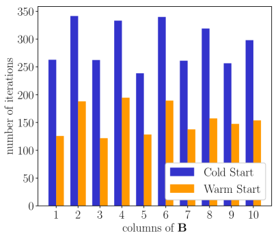
Figure 2: Average BFGS iterations for each subproblem across the columns.

Updating _j can be done efficiently by exploiting the optimized DMD problem structure. In particular, BFGS builds a Hessian approximation as it proceeds. All of the subproblems for _j share the same ${\boldsymbol{\Phi}}({\boldsymbol{\alpha}})$ and, since the columns of ${\mathbf{B}}$ contain spatial information, neighboring columns are likely to be similar to each other. After solving subproblem $j$, we use the resulting Hessian approximation to initialize the next subproblem $j+1$. Warm starts cut total BFGS iterations in half, see Figure 2.

There are different ways to update the weights ${\mathbf{w}}$, see line 4 in Algorithms 1 and 2. Define

$$\rho_{j}^{\nu}=\rho\left(X_{\cdot j}-{\boldsymbol{\Phi}}({\boldsymbol{\alpha}}^{\nu})_{j}^{\nu+1}\right).$$

The objective with respect to ${\mathbf{w}}$ is given by

$$\min_{{\mathbf{w}}}\sum_{j=1}^{n}w_{j}\rho_{j}^{\nu}+s({\mathbf{w}}),$$

where $s$ encodes the weight constraints (11). The simplest update rule is to set $w_{j}=1$ if $\rho_{j}^{\nu}$ is one of the $h$ smallest, and $0$ otherwise (Yang et al., 2016); this corresponds to partial minimization in ${\mathbf{w}}$ at every step. A less aggressive strategy is to use proximal updates on ${\mathbf{w}}$,

$${\mathbf{w}}^{\nu+1}=\mbox{prox}_{\eta_{\mathbf{w}}s}\left({\mathbf{w}}^{\nu}-\eta_{\mathbf{w}}\nabla_{\mathbf{w}}f({\boldsymbol{\alpha}}^{\nu},{\mathbf{B}}^{\nu+1},{\mathbf{w}}^{\nu})\right)$$

where any step size $\eta_{\mathbf{w}}>0$ can be used (Aravkin and Davis, 2016). We use the former simple rule as the default in the algorithm. When $h=n$, trimming is turned off, and all weights are identically equal to $1$.

Algorithm 3 SVRG for DMD

1:${\boldsymbol{\alpha}}^{0}$, ${\mathbf{B}}^{0}$, ${\mathbf{w}}^{0}$

2:Initialize $\nu=0$, $\zeta_{j}=\nabla f_{j}\left({\boldsymbol{\alpha}}^{0},{\mathbf{w}}^{0}\right)$ for $j=1,2,\ldots,n$, and $\zeta=\frac{1}{n}\sum_{j=1}^{n}\zeta_{j}$

3:while not converged do

4:     Uniformly sample $I^{\nu}\subset\{1,2,\ldots,n\}$, such that $\left|I^{\nu}\right|=\tau$

5:     Sample $J^{\nu}\in\{0,1\}$, such that $P(J=1)\ll P(J=0)$.

6:     for $j\in I_{\nu}$ do

7:         ${}^{\nu+1}_{j}$ $\leftarrow$ $\displaystyle\arg\min_{w}{}_{j}^{\nu}\rho(X_{\cdot,j}-{\boldsymbol{\Phi}}({\boldsymbol{\alpha}}^{\nu}))+q()$

8:         $\zeta_{j}^{+}$ $\leftarrow$ $\nabla\tilde{g}_{j}\left({\boldsymbol{\alpha}}^{\nu},{\mathbf{w}}\right)$      

9:     if $J=1$ then

10:         ${\mathbf{w}}^{\nu+1}$ $\leftarrow$ weights update

11:     else

12:         ${\mathbf{w}}^{\nu+1}$ $\leftarrow$ ${\mathbf{w}}^{\nu}$      

13:     ${\boldsymbol{\alpha}}^{\nu+1}$ $\leftarrow$ $\text{prox}_{\eta_{\boldsymbol{\alpha}}r}\left({\boldsymbol{\alpha}}^{\nu}-\eta_{\boldsymbol{\alpha}}\left[\frac{1}{\tau}\sum_{j\in I^{\nu}}\left(\zeta_{j}^{+}-\zeta_{j}\right)+\zeta\right]\right)$

14:     $\eta_{\boldsymbol{\alpha}}$ $\leftarrow$ step size update

15:     $\zeta_{j}$ $\leftarrow$ $\zeta_{j}^{+}$ for $j\in I^{\nu}$

16:     $\zeta$ $\leftarrow$ $\frac{1}{n}\sum_{j=1}^{n}\zeta_{j}$

17:     $\nu$ $\leftarrow$ $\nu+1$

18:${\boldsymbol{\alpha}}^{\nu}$, ${\mathbf{B}}^{\nu}$

3.3 A scalable stochastic method

In DMD applications, $n$ represents the number of spatial variables, and is often much larger than either $m$ or $k$. Therefore, step 2 of Algorithms 1 and 2 is a computational bottleneck. We use stochastic methods to scale the approach. The basic idea is to partially minimize over a random sample of the columns of ${\mathbf{B}}$; the resulting (scaled) gradient is an unbiased estimate of $\nabla_{{\boldsymbol{\alpha}}}\tilde{f}$. More precisely, define

$${}_{j}({\boldsymbol{\alpha}},{\mathbf{w}}) =\operatorname*{argmin}_{w}{}_{j}\rho\left(X_{\cdot j}-{\boldsymbol{\Phi}}({\boldsymbol{\alpha}})\right)+q(),$$

$$\tilde{g}_{j}({\boldsymbol{\alpha}},{\mathbf{w}}) =w_{j}\rho(X_{\cdot j}-{\boldsymbol{\Phi}}({\boldsymbol{\alpha}})_{j}({\boldsymbol{\alpha}},{\mathbf{w}}))+q(_{j}({\boldsymbol{\alpha}},{\mathbf{w}})).$$

Then we have

$$\tilde{f}({\boldsymbol{\alpha}},{\mathbf{w}})=\sum_{j=1}^{n}\tilde{g}_{j}({\boldsymbol{\alpha}},{\mathbf{w}})+r({\boldsymbol{\alpha}})+s({\mathbf{w}}).$$

This is a classical setting for stochastic methods. In each iteration, we can use a subset of $\tilde{g}_{j}$ to calculate the approximate gradient for the smooth part of $\tilde{f}$ in order to reduce the computational burden. Here we use SVRG (Johnson and Zhang, 2013) as our stochastic solver for the outer problem; the full details are given in Algorithm 3. Note that this stochastic approach is an alternative to using a cost reduction based on projecting onto SVD modes (Askham and Kutz, 2017) or using an optimized but fixed subsampling of the columns (Guéniat et al., 2015). With the method of Algorithm 3, none of the data is discarded or filtered by the cost reduction procedure.

In Figure 3, we solve a problem with dimension $m=512$ and $n=1000$. A diminishing step size scheme is used, taking

$$\eta_{\boldsymbol{\alpha}}^{\nu}=\frac{\eta_{\boldsymbol{\alpha}}^{0}}{\mbox{floor}(\nu/K)+1},$$

with $\eta^{0}_{\boldsymbol{\alpha}}=10^{-7}$ and $K=500$ for the result in Figure 3. Comparing the algorithms according to total _j subproblems, we see that SVRG decreases faster and is less noisy than the Stochastic Proximal Gradient (SPG) method. Proximal Gradient (PG) decreases quickly in the beginning, but is soon overtaken by stochastic methods. SVRG gives a significant improvement over SPG.

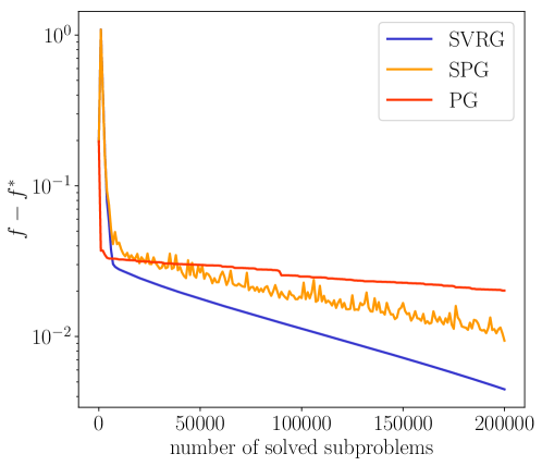
Figure 3: Compare performance of SVRG, Stochastic Proximal Gradient (SPG) method and Proximal Gradient (PG) method over the same data set.

The trimming weights ${\mathbf{w}}$ rely on global information; that is, the best $h$ residuals are easily selected after all of the residuals have been calculated. This is why the weights update (lines 8-11 of Algorithm 3) is done rarely. For detailed analysis of stochastic algorithms with trimming, see Aravkin and Davis (2016).

4 Synthetic examples

In this section, we examine the performance of the robust DMD on a pair of synthetic test cases with known solution. These examples are drawn from the additive noise study of Dawson et al. (2016).

4.1 A simple periodic example

Let ${\mathbf{x}}(t)$ be the solution of a two dimensional linear system with the following dynamics

$$\dot{{\mathbf{x}}}=\begin{pmatrix}1&-2\\ 1&-1\end{pmatrix}{\mathbf{x}}\;.$$ (17)

We use the initial condition ${\mathbf{x}}(0)=(1,0.1)^{\intercal}$ and take snapshots

$${\mathbf{x}}_{j}={\mathbf{x}}(j\Delta t)+\sigma{\mathbf{g}}_{j}+\mu{\mathbf{s}}_{j}\,,$$

where $\Delta t=0.1$, $\sigma$ and $\mu$ are prescribed noise levels, ${\mathbf{g}}_{j}$ is a vector whose entries are drawn from a standard normal distribution, and ${\mathbf{s}}_{j}$ is a vector whose entries are the product of a Bernoulli trial with small expectation $p$ and a standard normal (corresponding to sparse noise). The snapshots are therefore corrupted with a base level of noise $\sigma$ and sparse “spikes” of size $\mu$ with firing rate $p$. A sample time series for this example can be found in Figure 4.

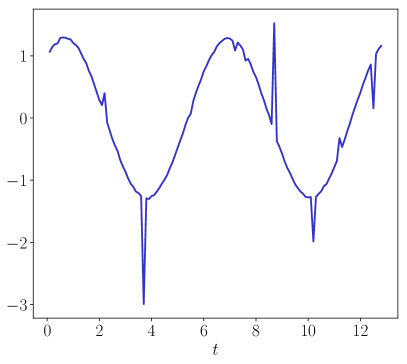
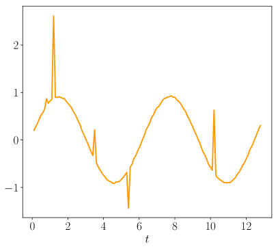
Figure 4: Sample time series of $x_{1}(t)$ and $x_{2}(t)$ for the simple periodic example, with background noise of size $\sigma=10^{-2}$ and spikes of size $\mu=1$ added at $p=5\%$ of the snapshots for each channel.

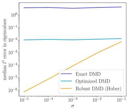
Figure 5: Median error in the computed eigenvalues over 200 runs. The background noise $\sigma$ varies while the size of the spikes is fixed at $\mu=1$ and the firing rate is fixed at $p=5\%$.

The $k=2$ eigenvalues of the system matrix in (17) are $\pm{\mathbf{i}}$, corresponding to sinusoidal dynamics in time. In Figure 5, we plot the median (over 200 random trials) of the $l^{1}$-norm error in the approximations of these eigenvalues using three different methods: the exact DMD of Tu et al. (2014); the optimized DMD as defined in (4); and the robust DMD as defined in (9), with $\rho$ the Huber norm and $h=n=2$ (no trimming). Each trial consists of the first 128 snapshots with additive noise. The level of the background noise, $\sigma$, varies over the experiments and the size and firing rate of the spikes are fixed at $\mu=1$ and $p=5\%$, respectively. We set the Huber parameter using knowledge of the problem set-up, i.e. $\kappa=5\sigma$, but in a real-data setting this parameter would have to be estimated or chosen adaptively. While the optimized DMD improves over the exact DMD, the error does not decrease as the level of the background noise decreases. We therefore see the effect of the sparse outliers using the optimized DMD. For the robust formulation, on the other hand, the accuracy of the eigenvalues is determined by the level of the background noise, so that the outliers are not biasing the computed eigenvalues.

4.2 An example with hidden dynamics

In the case that a signal contains some rapidly decaying components it can be more difficult to identify the dynamics, particularly in the presence of sensor noise (see Dawson et al., 2016). We consider a signal composed of two sinusoidal forms which are translating, with one growing and one decaying, i.e.

$$x(y,t)=\sin(k_{1}y-\omega_{1}t)e^{\gamma_{1}t}+\sin(k_{2}y-\omega_{2}t)e^{\gamma_{2}t}\;,$$ (18)

where $k_{1}=1$, $\omega_{1}=1$, $\gamma_{1}=1$, $k_{2}=0.4$, $\omega_{2}=3.7$, and $\gamma_{2}=-0.2$ (following settings used by Dawson et al. (2016)). This signal has $k=4$ continuous time eigenvalues given by $\gamma_{1}\pm i\omega_{1}$ and $\gamma_{2}\pm i\omega_{2}$. We set the domain of $y$ to be $[0,15]$ and use 300 equispaced points, $y_{j}$, to discretize. For the time domain, we set $\Delta t=\pi/(2^{8}-2)$ so that the number of snapshots we use, $m=2^{7}$, covers $[0,\pi/2]$. We denote the vector of discrete values $x(y_{j},t)$ by ${\mathbf{x}}(t)$. See Figure 6(a) for a surface plot of this data.

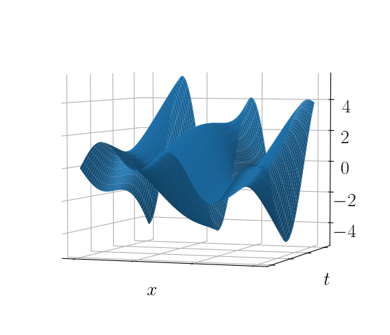
(a) clean data

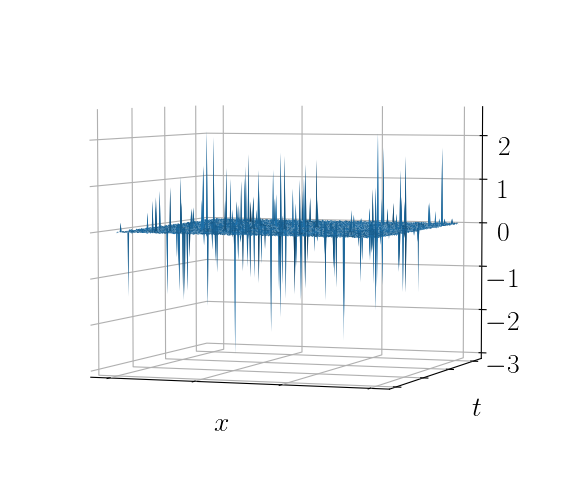
(b) “sparse noise”

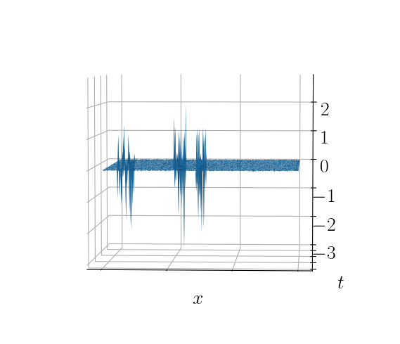
(c) “broken sensor”

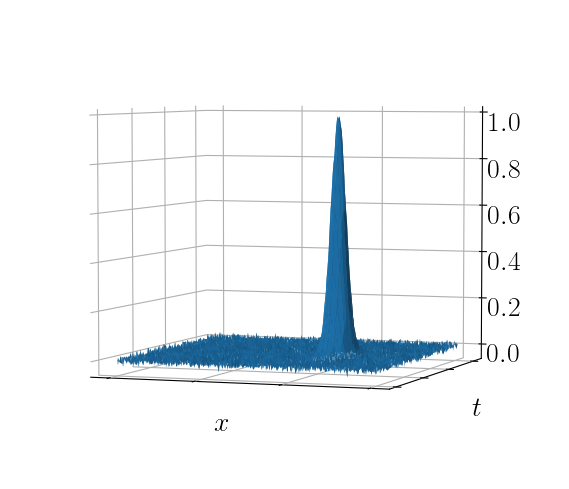
(d) “bump”

Figure 6: A surface plot of the data for the hidden dynamics example and surface plots of a sample of each type of noise we consider.

We consider three different types of perturbations of the data. The first perturbation adds background noise and spikes, as in the previous example, i.e. the snapshots are given by

$${\mathbf{x}}^{(1)}_{j}={\mathbf{x}}(j\Delta t)+\sigma{\mathbf{g}}_{j}+\mu{\mathbf{s}}_{j}\,,$$

where $\sigma$ and $\mu$ are prescribed noise levels, ${\mathbf{g}}_{j}$ is a vector whose entries are drawn from a standard normal distribution, and ${\mathbf{s}}_{j}$ is a vector whose entries are the product of a Bernoulli trial with small expectation $p$ and a standard normal. See Figure 6(b) for a sample plot of this “sparse noise” pattern. The second perturbation we consider adds background noise and spikes which are confined to specific entries of ${\mathbf{x}}_{j}$, i.e.

$${\mathbf{x}}^{(2)}_{j}={\mathbf{x}}(j\Delta t)+\sigma{\mathbf{g}}_{j}+\mu\tilde{{\mathbf{s}}}_{j}\,,$$

where ${\mathbf{g}}_{j}$, $\sigma$, and $\mu$ are as above and the $\tilde{\mathbf{s}}_{j}$ are sparse vectors which have the same sparsity pattern for all $j$ and nonzero entries drawn from a standard normal distribution (this corresponds to having a few broken sensors recording the data). We plot a sample of this “broken sensor” noise pattern in Figure 6(c). The third perturbation we consider adds background noise and a localized bump to the data, i.e.

$$\left[{\mathbf{x}}^{(3)}_{j}\right]_{i}=x(y_{i},j\Delta t)+\sigma\mathcal{N}(0,1)+A\exp\left(-\left(\frac{y_{b}-y_{i}}{w\Delta y}\right)^{2}-\left(\frac{t_{b}-j\Delta t}{w\Delta t}\right)^{2}\right)\,,$$

where $\sigma$ is as above, $\mathcal{N}(0,1)$ denotes a number drawn from the standard normal distribution, $A$ determines the maximum height of the bump, $w$ determines the “width” of the bump, and $y_{b}$ and $t_{b}$ determine the center of the bump in space and time (this corresponds to having some non-exponential dynamics in the data). In Figure 6(d), we plot a sample of this “bump” noise pattern.

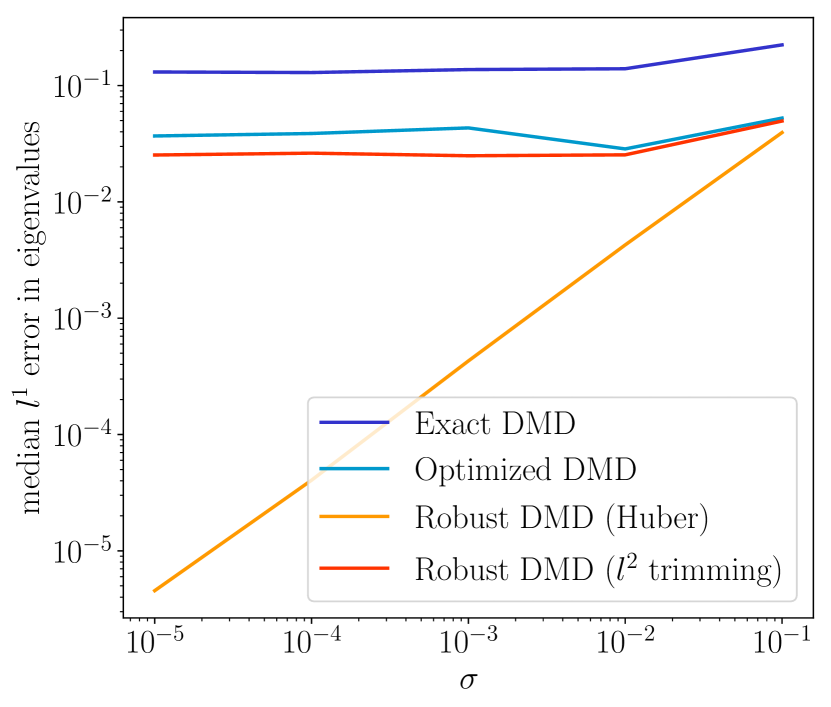
(a) “sparse noise”

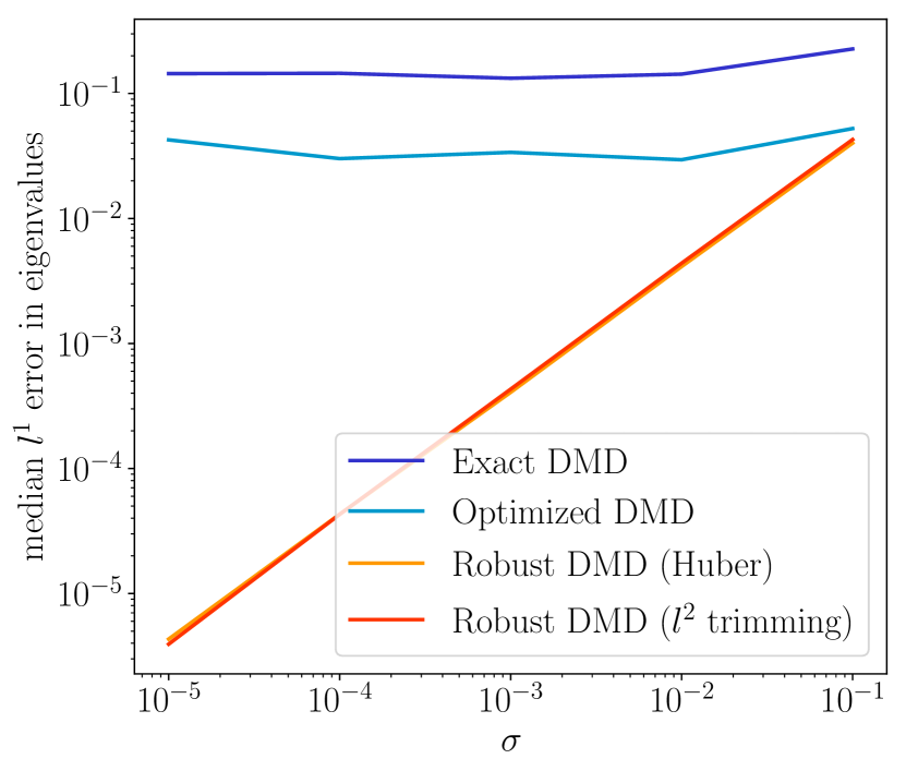
(b) “broken sensor”

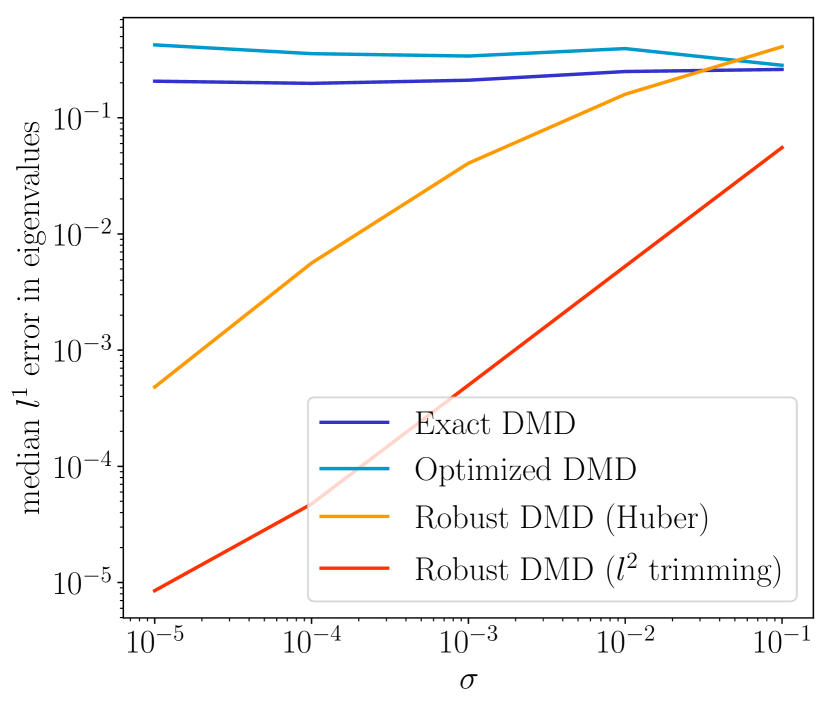
(c) “bump”

Figure 7: Median error in the computed eigenvalues over 200 runs. The background noise $\sigma$ varies while the size of the spikes is fixed at $\mu=1$ and the firing rate is fixed at $p=5\%$ for the “sparse noise” and “broken sensor” examples and the height is fixed at $A=1$ and the width at $w=10$ for the “bump” example.

In Figure 7, we plot the median (over 200 random trials) of the $l^{1}$-norm error in the approximations of the eigenvalues using four different methods: the exact DMD of Tu et al. (2014); the optimized DMD as defined in (4); the robust DMD as defined in (9), with $\rho$ the Huber norm and $h=n=300$ (no trimming); and the robust DMD with $\rho$ the standard Frobenius norm and $h=0.8n=240$ (trimming). Each trial consists of the first 128 snapshots with additive noise. The level of the background noise, $\sigma$, varies over the experiments. For the “sparse noise” and “broken sensor” snapshots, the size of the spikes is fixed at $\mu=1$ and the density is fixed at $p=5\%$, i.e. $5\%$ of the entries are corrupted for the “sparse noise” example and $5\%$ of the sensors are corrupted for the “broken sensor” example. For the “bump” snapshots, the height of the bump is fixed at $A=1$ and the width at $w=10$. We set the Huber parameter using knowledge of the problem set-up, i.e. $\kappa=5\sigma$, but in a real-data setting this parameter would have to be estimated or chosen adaptively.

With sparse noise, as in Figure 7(a), the results for the exact DMD, optimized DMD, and Huber norm-based robust DMD are consistent with the simple periodic example. The Huber norm formulation is the only one which is able to take advantage of the lower levels of background noise. The trimming formulation provides very little advantage for this example, as any sensor can be affected by the outliers. In contrast, we see that the trimming formulation is able to perform as well as the Huber formulation for the broken sensor example (see Figure 7(b)), as the algorithm is able to adaptively remove the broken sensors from the data. In Figure 7(c), we plot the results for the bump data, which display some interesting behavior. The optimized DMD actually performs worse than the exact DMD, which is attributable to over-fitting. For all but the highest background noise level, the Huber and trimming formulations show a significant advantage over the optimized DMD and exact DMD, with the trimming formulation performing the best. The trimming formulation therefore presents an attractive solution for data with unknown, localized deviations from the exponential basis of the DMD, especially given that the inner problem for trimming with the Frobenius penalty can be solved rapidly. Of course, trimming can be combined with a Huber (or other robust) penalty for increased robustness to outliers.

5 Real data examples

These examples will be added to a future draft.

5.1 Atmospheric chemistry data

5.2 Fluid simulation data

6 Conclusion and future directions

We have presented an optimization framework and a suite of numerical algorithms for computing the dynamic mode decomposition with robust penalties and parameter constraints. This framework allows for improved performance of the DMD in a number of settings, as borne out by synthetic and real data experiments. In the presence of sparse noise or non-exponential structure, the use of robust penalties significantly decreases the bias in the computed eigenvalues. When using the DMD to perform future state prediction, adding the constraint that the eigenvalues lie in the left half-plane increases the stability of the extrapolation. The algorithms presented are capable of solving small to medium-sized problems in seconds on a laptop and scale well to higher-dimensional problems due to their intrinsic parallelism and the efficiency of the SVRG approach. In contrast with previous approaches, the SVRG increases efficiency without throwing out data or incidentally filtering it. We believe that the framework and algorithms presented here will enable practitioners of the DMD to tackle larger, noisier, and more complex data sets than previously possible. The authors commit to releasing the software used for these calculations as an open-source package in the Julia language (Bezanson et al., 2012).

The present work can be extended in a number of ways. Because the inner solve completely decouples over the columns of ${\bf X}$ and ${\bf B}$, the algorithms presented above immediately generalize to data-sets with missing entries and even data which are collected asynchronously across sensors. While the global nature of an optimized DMD fit has advantages in terms of the quality of the recovered eigenvalues, it implicitly rules out process noise. However, including process noise or a known forcing term would be useful in many applications. Incorporating such terms into this optimization framework is ongoing work and results will be reported at a later date. We also note that much of the above applies to dimensionality reduction using any parameterized family of time dynamics, not just exponentials. For such an application, many of the algorithms above could be easily adapted, so long as gradient formulas are available.

Acknowledgments

T. Askham and J. N. Kutz acknowledge support from the Air Force Office of Scientific Research (FA9550-15-1-0385). J. N. Kutz also acknowledges support from the Defense Advanced Research Projects Agency (DARPA contract HR0011-16-C-0016). The work of A. Aravkin and P. Zheng was supported by the Washington Research Foundation Data Science Professorship.

References

- Aravkin and Davis (2016) Aleksandr Aravkin and Damek Davis. A SMART stochastic algorithm for nonconvex optimization with applications to robust machine learning. arXiv preprint arXiv:1610.01101, 2016.
- Aravkin and Van Leeuwen (2012) Aleksandr Y Aravkin and Tristan Van Leeuwen. Estimating nuisance parameters in inverse problems. Inverse Problems, 28(11):115016, 2012.
- Aravkin et al. (2017) Aleksandr Y Aravkin, Dmitriy Drusvyatskiy, and Tristan van Leeuwen. Efficient quadratic penalization through the partial minimization technique. IEEE Transactions on Automatic Control, 2017.
- Askham and Kutz (2017) Travis Askham and J Nathan Kutz. Variable projection methods for an optimized dynamic mode decomposition. arXiv preprint arXiv:1704.02343, 2017.
- Beck and Teboulle (2009) Amir Beck and Marc Teboulle. A fast iterative shrinkage-thresholding algorithm for linear inverse problems. SIAM journal on imaging sciences, 2(1):183–202, 2009.
- Bell and Burke (2008) Bradley M Bell and James V Burke. Algorithmic differentiation of implicit functions and optimal values. Advances in Automatic Differentiation, pages 67–77, 2008.
- Bezanson et al. (2012) Jeff Bezanson, Stefan Karpinski, Viral B Shah, and Alan Edelman. Julia: A fast dynamic language for technical computing. arXiv preprint arXiv:1209.5145, 2012.
- Brunton et al. (2016) B. W. Brunton, L. A. Johnson, J. G. Ojemann, and J. N. Kutz. Extracting spatial–temporal coherent patterns in large-scale neural recordings using dynamic mode decomposition. Journal of Neuroscience Methods, 258:1–15, 2016.
- Candès et al. (2011) Emmanuel J Candès, Xiaodong Li, Yi Ma, and John Wright. Robust principal component analysis? Journal of the ACM (JACM), 58(3):11, 2011.
- Chen et al. (2012) Kevin K Chen, Jonathan H Tu, and Clarence W Rowley. Variants of dynamic mode decomposition: boundary condition, koopman, and fourier analyses. Journal of nonlinear science, 22(6):887–915, 2012.
- Combettes and Pesquet (2011) Patrick L Combettes and Jean-Christophe Pesquet. Proximal splitting methods in signal processing. In Fixed-point algorithms for inverse problems in science and engineering, pages 185–212. Springer, 2011.
- Cunningham and Ghahramani (2015) John P Cunningham and Zoubin Ghahramani. Linear dimensionality reduction: survey, insights, and generalizations. Journal of Machine Learning Research, 16(1):2859–2900, 2015.
- Dawson et al. (2016) Scott TM Dawson, Maziar S Hemati, Matthew O Williams, and Clarence W Rowley. Characterizing and correcting for the effect of sensor noise in the dynamic mode decomposition. Experiments in Fluids, 57(3):1–19, 2016.
- Dicle et al. (2016) Caglayan Dicle, Hassan Mansour, Dong Tian, Mouhacine Benosman, and Anthony Vetro. Robust low rank dynamic mode decomposition for compressed domain crowd and traffic flow analysis. In Multimedia and Expo (ICME), 2016 IEEE International Conference on, pages 1–6. IEEE, 2016.
- Erichson et al. (2015) N Benjamin Erichson, Steven L Brunton, and J Nathan Kutz. Compressed dynamic mode decomposition for real-time object detection. Preprint, 2015.
- Golub and LeVeque (1979) G. H. Golub and R. J. LeVeque. Extensions and uses of the variable projection algorithm for solving nonlinear least squares problems. In Proceedings of the 1979 Army Numerical Analsysis and Computers Conference, 1979.
- Grosek and Kutz (2014) J. Grosek and J. N. Kutz. Dynamic Mode Decomposition for Real-Time Background/Foreground Separation in Video. arXiv preprint, arXiv:1404.7592, 2014.
- Guéniat et al. (2015) Florimond Guéniat, Lionel Mathelin, and Luc R. Pastur. A dynamic mode decomposition approach for large and arbitrarily sampled systems. Physics of Fluids, 27(2):025113, 2015. doi: 10.1063/1.4908073. URL http://dx.doi.org/10.1063/1.4908073.
- Hemati et al. (2017) Maziar S Hemati, Clarence W Rowley, Eric A Deem, and Louis N Cattafesta. De-biasing the dynamic mode decomposition for applied koopman spectral analysis of noisy datasets. Theoretical and Computational Fluid Dynamics, pages 1–20, 2017.
- Huber (2011) Peter J Huber. Robust statistics. In International Encyclopedia of Statistical Science, pages 1248–1251. Springer, 2011.
- Johnson and Zhang (2013) Rie Johnson and Tong Zhang. Accelerating stochastic gradient descent using predictive variance reduction. In Advances in neural information processing systems, pages 315–323, 2013.
- Kutz et al. (2016) J Nathan Kutz, Steven L Brunton, Bingni W Brunton, and Joshua L Proctor. Dynamic Mode Decomposition: Data-Driven Modeling of Complex Systems. SIAM, 2016.
- Locantore et al. (1999) N Locantore, JS Marron, DG Simpson, N Tripoli, JT Zhang, KL Cohen, Graciela Boente, Ricardo Fraiman, Babette Brumback, Christophe Croux, et al. Robust principal component analysis for functional data. Test, 8(1):1–73, 1999.
- Maronna et al. (2006) RARD Maronna, R Douglas Martin, and Victor Yohai. Robust statistics. John Wiley & Sons, Chichester. ISBN, 2006.
- Rockafellar and Wets (2009) R Tyrrell Rockafellar and Roger J-B Wets. Variational analysis, volume 317. Springer Science & Business Media, 2009.
- Rousseeuw (1985) Peter J Rousseeuw. Multivariate estimation with high breakdown point. Mathematical statistics and applications, 8:283–297, 1985.
- Schmid and Sesterhenn (2008) P. J. Schmid and J. Sesterhenn. Dynamic mode decomposition of numerical and experimental data. In 61st Annual Meeting of the APS Division of Fluid Dynamics. American Physical Society, November 2008.
- Schmid (2010) Peter J Schmid. Dynamic mode decomposition of numerical and experimental data. Journal of fluid mechanics, 656:5–28, 2010.
- Takeishi et al. (2017) Naoya Takeishi, Yoshinobu Kawahara, Yasuo Tabei, and Takehisa Yairi. Bayesian dynamic mode decomposition. In Proc. of the 26th Int’l Joint Conf. on Artificial Intelligence (IJCAI), pages 2814–2821, 2017.
- Tu et al. (2014) Jonathan H Tu, Clarence W Rowley, Dirk M Luchtenburg, Steven L Brunton, and J Nathan Kutz. On dynamic mode decomposition: Theory and applications. Journal of Computational Dynamics, 1(2):391–421, 2014.
- Wright et al. (2009) John Wright, Arvind Ganesh, Shankar Rao, Yigang Peng, and Yi Ma. Robust principal component analysis: Exact recovery of corrupted low-rank matrices via convex optimization. In Advances in neural information processing systems, pages 2080–2088, 2009.
- Yang et al. (2016) Eunho Yang, Aurelie Lozano, and Aleksandr Aravkin. High-dimensional trimmed estimators: A general framework for robust structured estimation. arXiv preprint arXiv:1605.08299, 2016.