Crossover between the Gaussian orthogonal ensemble, the Gaussian unitary ensemble, and Poissonian statistics

Abstract

Until now only for specific crossovers between Poissonian statistics (P), the statistics of a Gaussian orthogonal ensemble (GOE), or the statistics of a Gaussian unitary ensemble (GUE) analytical formulas for the level spacing distribution function have been derived within random matrix theory. We investigate arbitrary crossovers in the triangle between all three statistics. To this aim we propose an according formula for the level spacing distribution function depending on two parameters. Comparing the behavior of our formula for the special cases of P$\rightarrow$GUE, P$\rightarrow$GOE, and GOE$\rightarrow$GUE with the results from random matrix theory, we prove that these crossovers are described reasonably. Recent investigations by F. Schweiner et al. [Phys. Rev. E 95, 062205 (2017)] have shown that the Hamiltonian of magnetoexcitons in cubic semiconductors can exhibit all three statistics in dependence on the system parameters. Evaluating the numerical results for magnetoexcitons in dependence on the excitation energy and on a parameter connected with the cubic valence band structure and comparing the results with the formula proposed allows us to distinguish between regular and chaotic behavior as well as between existent or broken antiunitary symmetries. Increasing one of the two parameters, transitions between different crossovers, e.g., from the P$\rightarrow$GOE to the P$\rightarrow$GUE-crossover, are observed and discussed.

I Introduction

It is now widely accepted that classical chaotic dynamics manifests itself in the statistical quantities of the corresponding quantum system Rao and Taylor (2002); Mehta (2004); Porter (1965). All systems with a Hamiltonian leading to global chaos in the classical dynamics can be assigned to one of three universality classes: the orthogonal, the unitary or the symplectic universality class Haake (2010). To which of these universality classes a given system belongs is determined by the remaining symmetries of the system. Many physical systems are invariant under time-reversal or possess at least one remaining antiunitary symmetry. These systems show the statistics of a Gaussian orthogonal ensemble (GOE). Only if all antiunitary symmetries are broken, the statistics of a Gaussian unitary ensemble (GUE) occurs. The Gaussian symplectic ensemble will not be treated here and is described, e.g., in Ref. Haake (2010). Until now only few physical systems are known showing a crossover between GOE and GUE statistics in dependence on the system parameters: the kicked top Haake et al. (1987), the Anderson model Shukla (2005), and magnetoexcitons in cubic semiconductors Schweiner et al. (2017a); Aßmann et al. (2016). While the kicked top is a time-dependent system, which has to be treated within Floquet theory Lenz and Haake (1991); Haake et al. (1987), and the Anderson model is rather a model system for a $d$-dimensional disordered lattice Shukla (2005), we showed in Ref. Schweiner et al. (2017b) that magnetoexcitons, i.e., excitons in magnetic fields, are a realistic physical system perfectly suitable to study crossovers between the Poissonian (P) level statistics, which describes the classically integrable case, GOE statistics, and GUE statistics.

Only for the specific crossovers of P$\rightarrow$GOE, P$\rightarrow$GUE, and GOE$\rightarrow$GUE analytical formulas for the level spacing distribution function have been derived within random matrix theory Schierenberg et al. (2012). We have recently investigated the crossovers P$\rightarrow$GUE and GOE$\rightarrow$GUE for magnetoexcitons Schweiner et al. (2017b) and obtained a very good agreement with these functions. However, what has not been investigated so far are arbitrary crossovers in the triangle between all three statistics in dependence on two of the system parameters. In this paper we will investigate these crossovers in dependence on the energy and one of the Luttinger parameters, which describes the cubic warping of the valence bands in a semiconductor. Within random matrix theory it would be, in principle, possible to derive an analytical formula which describes these arbitrary crossovers and with which our results for magnetoexcitons could be compared. However, this derivation is very challenging and beyond the scope of the present work. On the other hand, crossovers between different symmetry classes are not universal Kunstman et al. (1997). Hence, we propose a function with two parameters for arbitrary crossovers and show that it describes these crossovers reasonably well by comparing it for the special cases of P$\rightarrow$GOE, P$\rightarrow$GUE, and GOE$\rightarrow$GUE with the analytical formulas known. We choose the two parameters such that one describes the crossover from regular to irregular behavior and that the other one describes the breaking of antiunitary symmetries. Hence, by evaluating the numerical results with the function proposed, we can distinguish between regular and chaotic behavior as well as between existent or broken antiunitary symmetries. Varying one of the two control parameters allows us to observe and discuss transitions between different crossovers, e.g., from the P$\rightarrow$GOE to the P$\rightarrow$GUE-crossover.

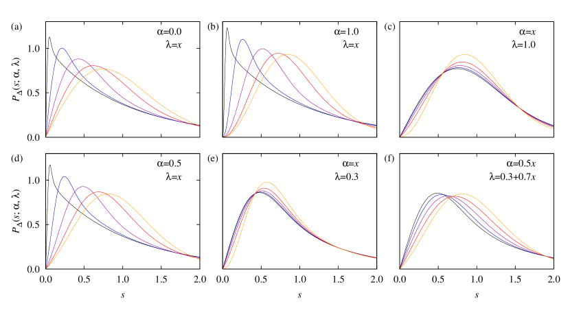
Figure 1: The crossover function $P_{\triangle}(s;\,\alpha,\,\lambda)$ of Eq. (10) for different combinations of the parameters $\alpha$ and $\lambda$. The values of these parameters are given according to the linear equations in each panel with $x=0.02,\,0.10,\,0.25,\,0.5,\,1.0$ (from dark to bright or left to right). 

The paper is organized as follows: In Sec. II we propose the function for arbitrary crossovers in the triangle P-GOE-GUE and compare it with the results from random matrix theory for specific crossovers. After a short discussion of the model system of magneoexcitons in cubic semiconductors in Sec. III, we present a comprehensive discussion of the numerical results for all possible crossovers in the triangle in Sec. IV. Finally, we give a short summary and outlook in Sec. V.

II Crossover functions

In this section we propose a formula for arbitrary crossovers in the triangle of Poissonian, GOE and GUE statistics. For crossovers between each two of the statistics analytical formulas have been derived within random matrix theory in Ref. Schierenberg et al. (2012). They investigated the statistical properties of a $2\times 2$ random matrix of the form

$$H=H_{\beta}+\lambda H_{\beta^{\prime}}$$ (1)

with a coupling parameter $\lambda$. $H_{\beta^{\prime}}$ describes the perturbation breaking the symmetry of the original system $H_{\beta}$. The Poisson process is defined by

$$H_{0}=\left(\begin{array}[]{cc}0&0\\ 0&p\end{array}\right)$$ (2)

with a Poisson-distributed non-negative random number $p$. The GOE process and the GUE process are described by a real symmetric matrix

$$H_{1}=\left(\begin{array}[]{cc}a&c\\ c&b\end{array}\right)$$ (3)

and a complex Hermitian matrix

$$H_{2}=\left(\begin{array}[]{cc}a&c_{0}+ic_{1}\\ c_{0}-ic_{1}&b\end{array}\right),$$ (4)

respectively. A detailed evaluation of the level spacing distribution yields the probability densities to find two neighboring eigenvalues at a distance $s$ Schierenberg et al. (2012): $P_{\mathrm{P}\rightarrow\mathrm{GOE}}(s;\,\lambda)$, $P_{\mathrm{P}\rightarrow\mathrm{GUE}}(s;\,\lambda)$, and $P_{\mathrm{GOE}\rightarrow\mathrm{GUE}}(s;\,\lambda)$. These formulas are presented in detail in Refs. Schierenberg et al. (2012); Schweiner et al. (2017b). It is important to note that the parameter $\lambda$ can have all values between $0$ and $\infty$. However, already for $\lambda\approx 1$ the crossover to the statistics of lower symmetry is almost completed Schweiner et al. (2017b).

For the most general case of arbitrary crossovers between the three processes, one would have to choose the ansatz

$$H=H_{0}+\lambda_{1}H_{1}+\lambda_{2}H_{2}$$ (5)

to derive the nearest-neighbor spacing distribution $P_{\mathrm{P}-\mathrm{GOE}-\mathrm{GUE}}(s;\,\lambda_{1};\,\lambda_{2})$. However, as already the exact analytical calculations of Ref. Schierenberg et al. (2012) are very complicated, we here present a different approach.

We already stated in the introduction that the crossover between different symmetry classes is not universal. Besides the crossover formulas derived within random matrix theory there are also other interpolating distributions, e.g., for the crossover $\mathrm{P}\rightarrow\mathrm{GOE}$, which have been proposed in the literature Berry and Robnik (1984); Brody (1973); Caurier et al. (1990); Hasegawa et al. (1988); Izrailev (1990). Hence, we also propose a new formula for the arbitrary crossovers based on the formulas of random matrix theory. We define the function

$$P_{\triangle}(s;\,\alpha,\,\lambda) \equiv P_{\mathrm{P}-\mathrm{GOE}-\mathrm{GUE}}(s;\,\alpha;\,\lambda)$$ (6)

$$= (1-\alpha)P_{\mathrm{P}\rightarrow\mathrm{GOE}}(s;\,\lambda)$$

$$+\alpha P_{\mathrm{P}\rightarrow\mathrm{GUE}}(s;\,\lambda),$$

which is normalized

$$\int_{0}^{\infty}\,\mathrm{d}s\,P_{\triangle}(s;\,\alpha,\,\lambda)=(1-\alpha)+\alpha=1$$ (7)

and fulfils the condition

$$\int_{0}^{\infty}\,\mathrm{d}s\,sP_{\triangle}(s;\,\alpha,\,\lambda)=(1-\alpha)+\alpha=1$$ (8)

for the mean spacing. In Fig. 1 we show the function $P_{\triangle}(s;\,\alpha,\,\lambda)$ for different values of $\alpha$ and $\lambda$.

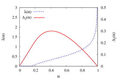
Figure 2: The optimum values of the parameter $\lambda$ when fitting $P_{\mathrm{GOE}\rightarrow\mathrm{GUE}}(s;\,\lambda)$ to $P_{\triangle}(s;\,\alpha,\,10)$ for given values of $\alpha$. With these values the distance $\Delta_{2}$ has been calculated according to Eq. (9). For further information see text. 

It can be easily seen that this function correctly describes the crossovers P$\rightarrow$GOE (for $\alpha=0$) and P$\rightarrow$GUE (for $\alpha=1$). When setting $\lambda\gg 1$ and increasing $\alpha$ from $0$ to $1$ this function should also describe the remaining crossover GOE$\rightarrow$GUE. Therefore, we fit the function $P_{\mathrm{GOE}\rightarrow\mathrm{GUE}}(s;\,\lambda)$ from random matrix theory to $P_{\triangle}(s;\,\alpha,\,10)$ for given values of $\alpha$ using $\lambda$ as a fit parameter (cf. Refs. Schierenberg et al. (2012); Schweiner et al. (2017b), where the maximum value of $\lambda$ is 10). For the optimum values $\lambda(\alpha)$, we then calculate the $L_{2}$ distance

$$\Delta_{2}(\alpha) = \left[\int_{0}^{\infty}\,\mathrm{d}s\,\left[P_{\mathrm{GOE}\rightarrow\mathrm{GUE}}(s;\,\lambda(\alpha))\right.\right.$$ (9)

$$\qquad\qquad\left.\phantom{\int_{0}^{\infty}}\left.-P_{\triangle}(s;\,\alpha,\,1)\right]^{2}\right]^{1/2}$$

as a measure of the fit quality Schierenberg et al. (2012). The results for $\Delta_{2}(\alpha)$ and $\lambda(\alpha)$ are shown in Fig. 2. It can be seen that the value of $\lambda$ grows monotonically for increasing values of $\alpha$ and that $\Delta_{2}(\alpha)$ approaches zero for $\alpha\rightarrow 0$ and $\alpha\rightarrow 1$, which describe the limiting cases of GOE and GUE statistics, respectively, Both observations indicate that our function $P_{\triangle}(s;\,\alpha,\,10)$ describes the crossover GOE$\rightarrow$GUE reasonably well. It is understandable that our function deviates from $P_{\mathrm{GOE}\rightarrow\mathrm{GUE}}(s;\,\lambda)$ for $0<\alpha<1$. For $\alpha\approx 0.4$ the deviation is largest with $\Delta_{2}\approx 0.3$. Due to these findings and the fact that crossover functions are not universal, we are certain that the function $P_{\triangle}(s;\,\alpha,\,\lambda)$ provides an adequate description of crossovers in the triangle of Poisson, GOE, and GUE statistics.

We finally note that the value of the parameter $\alpha$ in Eq. (10) is ambiguous for $\lambda=0$ since it is

$$P_{\triangle}(s;\,\alpha,\,0) = (1-\alpha)P_{\mathrm{P}}(s)+\alpha P_{\mathrm{P}}(s)=P_{\mathrm{P}}(s).$$ (10)

Hence, when having fitted the function $P_{\triangle}(s;\,\alpha,\,\lambda)$ to numerical results, we always present the product $\alpha\lambda$ instead of $\alpha$.

In Fig. 3 we show the triangle of Poissonian, GOE, and GUE statistics, which will be important when discussing the numerical results. Since we plot $\alpha\lambda$ against $\lambda$, the lower left corner corresponds to Poissonian statistics while the lower right corner and the upper right corner correspond to GOE statistics and GUE statistics, respectively. The green solid line shows the value of $\alpha=1$.

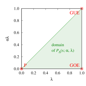
Figure 3: The triangle of the different statistics with Poissonian $(\lambda=0)$, GOE $(\alpha=0,\,\lambda=1)$, and GUE statistics $(\alpha=1,\,\lambda=1)$ located at the corners. The green area shows the domain of the function $P_{\triangle}(s;\,\alpha,\,\lambda)$ . 

III Magnetoexcitons

Excitons in semiconductors are fundamental quasi-particles, which are often regarded as the hydrogen analog of the solid state. They consist of a negatively charged electron in the conduction band and a positivley charged hole in the valence band interacting via a Coulomb interaction which is screened by the dielectric constant. Especially for cuprous oxide $\left(\mathrm{Cu_{2}O}\right)$ an almost perfect hydrogen-like absorption series has been observed for the yellow exciton up to a principal quantum number of $n=25$ Kazimierczuk et al. (2014). This remarkable high-resolution absorption experiment has opened the field of research of giant Rydberg excitons, and stimulated a large number of experimental and theoretical investigations Kazimierczuk et al. (2014); Aßmann et al. (2016); Freitag et al. (2017); Schweiner et al. (2016a); Grünwald et al. (2016); Feldmaier et al. (2016); Thewes et al. (2015); Schöne et al. (2016); Schweiner et al. (2016b, 2017c, 2017a); Heckötter et al. (2017a); Zielińska-Raczyńska et al. (2017); Schweiner et al. (2016c); Zielińska-Raczyńska et al. (2016a, b); Schweiner et al. (2017d, b, e, f, g); Schöne et al. (2017); Kurz et al. (2017); Semkat et al. (2017); Stielow et al. (2017); Heckötter et al. (2017b).

When treating excitons in magnetic fields, i.e., magnetoexcitons, it is indispensable to account for the complete cubic valence band structure of a semiconductor in a quantitative theory Schweiner et al. (2017c). Very recently, we have shown that this cubic valence band structure breaks all antiunitary symmetries Schweiner et al. (2017a) and that, depending on the system parameters, Poissonian, GOE and GUE statistics can be obeserved Schweiner et al. (2017b).

The Hamiltonian of magnetoexcitons has been discussed thoroughly in Refs. Schweiner et al. (2017c, b, e). In this paper we use the simplified model of magnetoexcitons of Ref. Schweiner et al. (2017b), in which the spins of the electron and the hole are neglected. Without the magnetic field the Hamiltonian of the relative motion between electron and hole reads in terms of irreducible tensors

$$H_{0} = -\frac{e^{2}}{4\pi\varepsilon_{0}\varepsilon}\frac{1}{r}+\frac{\gamma^{\prime}_{1}}{2\hbar^{2}m_{0}}\left[\frac{\delta^{\prime}}{3}\left(\sum_{k=\pm 4}\left[P^{(2)}\times I^{(2)}\right]_{k}^{(4)}\right.\right.$$

$$+ \left.\left.\frac{\sqrt{70}}{5}\left[P^{(2)}\times I^{(2)}\right]_{0}^{(4)}\right)+\hbar^{2}p^{2}-\frac{\mu^{\prime}}{3}P^{(2)}\cdot I^{(2)}\right]$$

with the dielectric constant $\varepsilon$ and the parameters $\gamma_{1}^{\prime}$, $\mu^{\prime}$ and $\delta^{\prime}$, which are connected to the Luttinger parameters of the semiconductor and describe the curvature of the uppermost valence bands Luttinger (1956); Uihlein et al. (1981); Schweiner et al. (2016b). The tensor operators correspond to the Cartesian operators of the relative momentum $\bm{p}$ and the quasi-spin $I=1$, which is connected with the three uppermost valence bands. The parameter $\delta^{\prime}$ is of particular importance since it describes the cubic warping of the valence bands and thus the breaking of the spherical symmetry of the remaining terms in the Hamiltonian. The magnetic field $\bm{B}$ can finally be introduced in the Hamiltonian $H_{0}$ via the minimal substitution Schweiner et al. (2017c).

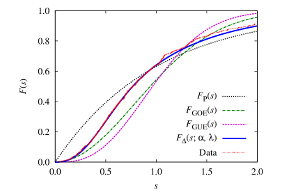
Figure 4: Cumulative distribution function for $\delta^{\prime}=-0.04$ and $\hat{E}=-0.6$. The numerical data (red linespoints) is fitted by the cumulative distribution function $F_{\triangle}(s;\,\alpha,\,\lambda)$ corresponding to the level spacing distribution of Eq. (10). The optimum fit parameters are here $\alpha=0.65$ and $\lambda=0.261$. Hence, the statistics is in the middle between Poissonian, GOE, and GUE statistics. 

We have shown in Refs. Schweiner et al. (2017a, b, e) that if the magnetic field is not oriented in one of the symmetry planes of the lattice, all antiunitary symmetries are broken unless $\delta^{\prime}=0$ holds. For the subsequent calculations we choose the orientation of $\bm{B}$ given by the angles $\varphi=\pi/8$ and $\vartheta=\pi/6$ in spherical coordinates, which is far away from the symmetry planes (cf. Ref. Schweiner et al. (2017b)).

We also use the method of a constant scaled energy known from atomic physics Wintgen (1987). Within this method the coordinate $r$, momentum $p$, and the energy $E$ are scaled by factor a $\gamma=B/B_{0}$ with $B_{0}=2.3505\times 10^{5}\,\mathrm{T}/(\gamma_{1}^{\prime 2}\varepsilon^{2})$ as described in detail in Ref. Schweiner et al. (2017b). The Schrödinger equation can then be written as a generalized eigenvalue problem

$$\bm{D}\bm{c}=\gamma^{1/3}\bm{M}\bm{c}$$ (12)

using the complete basis of Ref. Schweiner et al. (2017b). The matrices $\bm{D}$ and $\bm{M}$ and, hence, also the solutions of the Schrödinger equation depend on the two parameters $\hat{E}$ and $\delta^{\prime}$. It is well known from atomic physics that for small values of $\hat{E}$ the behavior of the system is regular while it becomes chaotic for larger values of $\hat{E}$. Consequently, $\hat{E}$ and $\delta^{\prime}$ are the important parameters when describing arbitrary crossovers in the triangle of Poissonian, GOE, and GUE statistics. We investigate the level spacing statistics of the eigenvalues of the Hamiltonian $H(\delta^{\prime},\,\hat{E})$ depending on these two parameters in the next section IV.

IV Results and discussion

Having solved the Schrödinger equation corresponding to the Hamiltonian $H(\delta^{\prime},\,\hat{E})$ of magnetoexcitons, we unfold the spectra according to the descriptions in Ref. Schweiner et al. (2017b) to obtain a constant mean spacing Wintgen and Friedrich (1987); Haake (2010); Bohigas et al. (1984); Brody et al. (1981). In doing so, we have to leave out a certain number of low-lying sparse levels to remove individual but nontypical fluctuations Wintgen and Friedrich (1987). Since the number of level spacings analyzed is comparatively small and comprises about $250$ to $500$ exciton states, we use the cumulative distribution function Grosa et al. (2014)

$$F(s)=\int_{0}^{s}P(x)\,\mathrm{d}x,$$ (13)

which is often more meaningful than histograms of the level spacing probability distribution function $P(s)$.

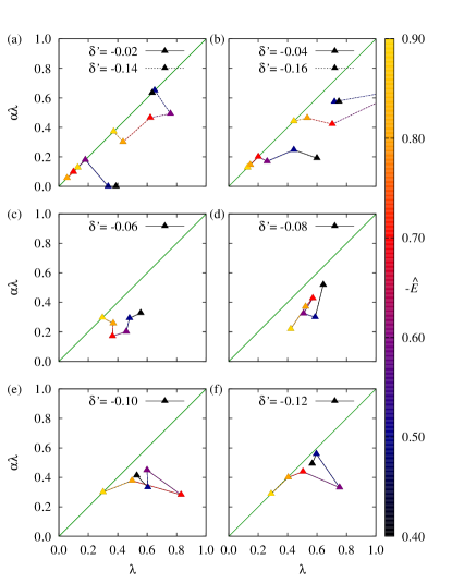
Figure 5: Resulting values for the parameters $\alpha\lambda$ and $\lambda$ when fitting the function $F_{\triangle}(s;\,\alpha,\,\lambda)$ corresponding to the level spacing distribution of Eq. (10) to the cumulative distribution function of the magnetoexciton. Here we show the behavior of the two fit parameters when keeping the value $\delta^{\prime}$ fixed (see label in the panels) and increasing the scaled energy $\hat{E}$ (color scale).  

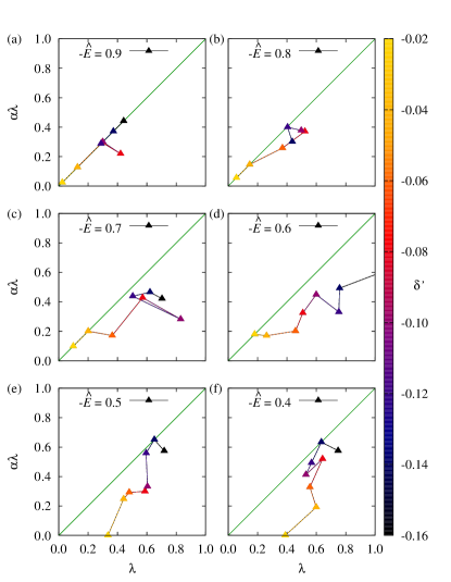
Figure 6: Same results as in Fig. 5 but shown for fixed values of the scaled energy $\hat{E}$ (see label in the panels) and decreasing values of $\delta^{\prime}$ (color scale).  

The numerical results are then fitted by the cumulative distribution function $F_{\triangle}(s;\,\alpha,\,\lambda)$ corresponding to the level spacing distribution of Eq. (10). This is shown exemplarily in Fig. 4. As can be seen, the agreement between the results and the function $F_{\triangle}(s;\,\alpha,\,\lambda)$ is reasonable. Note that this is generally true for all parameter sets. We evaluate numerical spectra for $\delta^{\prime}=-0.02,\,-0.04,\,\ldots,\,-0.16$ and $\hat{E}=-0.4,\,-0.5,\,\ldots,\,-0.9$.

The results for the fit parameters $\alpha$ and $\lambda$ are shown in Figs. 5 and 6. The two figures show the change in the fit parameters when keeping one of the two values $\delta^{\prime}$ and $\hat{E}$ fixed and varying the other one.

Let us start with Fig. 5 and the evaluation for fixed values of the parameter $\delta^{\prime}$. In the limit $\delta^{\prime}\rightarrow 0$ the influence of the cubic valence band structure vanishes and the system becomes hydrogen-like. It is well known that the hydrogen atom shows Poissonian statistics for small values of $\hat{E}$ and that a crossover to GOE statistics occurs when increasing the scaled energy Wintgen and Friedrich (1987). Hence, we expect for very small values of $|\delta^{\prime}|$ an almost horizontal line in the figures at small values of $\alpha\lambda$. This can be seen in Fig. 5 for $\delta^{\prime}=-0.02$ and even better for $\delta^{\prime}=-0.04$.

Here we already want to state that due to the comparatively small number of exciton states, which can be used in the numerical evaluation, the numerical data shows some fluctuations as can be seen, e.g., for larger values of $s$ in Fig. 4. Furthermore, when varying the parameters $\alpha$ and $\lambda$ only slightly, the shape of the function $P_{\triangle}(s;\,\alpha,\,\lambda)$ or $F_{\triangle}(s;\,\alpha,\,\lambda)$ hardly changes (cf. also Fig. 1). Consequently, due to these facts the results shown in Figs. 5 and 6 also show some fluctuations. However, one can nevertheless see the general behavior, when changing the $\delta^{\prime}$ and $\hat{E}$.

When increasing $|\delta^{\prime}|$ the cubic valence band structure becomes important and all antiunitary symmetries are broken. Hence, we see from Fig. 5 that the points are shifted towards higher values of $\alpha\lambda$ indicating that the line statistics becomes more and more GUE-like. We also observe that the line for fixed values of $\delta^{\prime}$ tends to change its shape from an almost horizontal line to a more diagonal line. The crossover for fixed values of $\delta^{\prime}$ and increasing $\hat{E}$ becomes more and more P$\rightarrow$GUE-like as expected.

Let us now turn to Fig. 6. We already observed in Ref. Schweiner et al. (2017b) that the parameter $\delta^{\prime}$ does not only break the remaining antiunitary symmetry of the hydrogen atom in external fields but also increases the chaotic behavior. When keeping the scaled energy $\hat{E}$ fixed at a very small value $\hat{E}=-0.9$ and increasing $\delta^{\prime}$, the statistics does not remain Poisson-like but the value of $\lambda$ already increases. Since $\alpha$ furthermore remains constant with $\alpha=1$, this indicates the crossover from Poissonian to GUE statistics. On the other hand, it is known from the hydrogen atom in external fields that when increasing $\hat{E}$ the behavior of the system becomes more and more chaotic, as well. For large values of $\hat{E}$ the system stays completely in the chaotic regime independent of the value of $\delta^{\prime}$. This can be seen in Fig. 6 for $\hat{E}=-0.4$, where the value of $\lambda$ is always larger than $0.4$. For $\hat{E}\geq-0.4$ the statistics is GOE-like in the hydrogen-like case with $\delta^{\prime}\rightarrow 0$. When increasing the value of $|\delta^{\prime}|$ it becomes more and more GUE-like as expected from the results of Ref. Schweiner et al. (2017a, b). Hence, we observe the crossover GOE$\rightarrow$GUE as an almost vertical line in the lower right panel of Fig. 6. For the intermediate values $-0.9\leq\hat{E}\leq-0.4$ of the scaled energy we observe the transition from the P$\rightarrow$GUE-crossover to the GOE$\rightarrow$GUE-crossover as a change in the lineshape from a diagonal to a more and more vertical line.

V Summary and outlook

We have proposed a new nearest-neighbor spacing distribution function, which allows to investigate arbitrary crossovers in the triangle of Poissonian, GOE, and GUE statistics. Comparing the behavior of this function for the special cases of P$\rightarrow$GOE, P$\rightarrow$GUE, and GOE$\rightarrow$GUE with the analytical formulas from random matrix theory, we could show that our function allows for a reasonable description of these crossovers. As excitons in external magnetic fields show all these statistics in dependence on the system parameters, they are ideally suited to investigate arbitrary crossovers between the three statistics. Evaluating numerical spectra for different values of the parameter $\delta^{\prime}$ and the scaled energy $\hat{E}$ we could observe transitions from the P$\rightarrow$GOE-crossover to the P$\rightarrow$GUE-crossover when increasing $\delta^{\prime}$ or from the P$\rightarrow$GUE-crossover to the GOE$\rightarrow$GUE-crossover when increasing $\hat{E}$.