Bootstrap estimators for the tail-index and for the count statistics of graphex processes

Abstract

Graphex processes resolve some pathologies in traditional random graph models, notably, providing models that are both projective and allow sparsity. Most of the literature on graphex processes study them from a probabilistic point of view. Techniques for inferring the parameter of these processes – the so-called graphon – are still marginal; exceptions are a few papers considering parametric families of graphons. Nonparametric estimation remains unconsidered. In this paper, we propose estimators for a selected choice of functionals of the graphon. Our estimators originate from the subsampling theory for graphex processes, hence can be seen as a form of bootstrap procedure.

1 Introduction

Many statistical models for relational data are based on vertex-exchangeable random graphs (also called graphon models), see [45] for a review. These models are interpretable and easy to work with, but have the considerable limitation that, almost surely, they generate dense graphs; that is, the number of edges scales quadratically with the number of vertices as the graph grows. Folk wisdom holds that real-world datasets are sparse and their degree distributions are power-law implying that graphon based approaches are unsatisfactory. Several model classes have been proposed to address this issue. A non exhaustive list includes edge exchangeable models [17], preferential attachement models [4], sparse graphon models [6, 7], and graphex processes [13, 52, 8].

Graphex processes have been proposed as a generalization of the graphon models that preserve the key properties, but allow for sparsity and degree distribution with power-law behaviour [13, 52, 14]. Thus, graphex processes are good candidates to model empirical graphs. Apart of [13, 51, 53, 29], inference on graphex processes is still marginal in the literature, most of papers studying graphex processes from a probabilistic point of view only. Efficient estimation remains challenging for these new models. The present paper intend to contribute to the study of graphex processes from a statistical viewpoint, driven by two main motivations described in section 2.

On a high-level, a graphex process $\{G_{t}\nonscript\,:\nonscript\,\mathopen{}\allowbreak t\geq 0\}$ is a graph-valued stochastic process. They are used as probabilitic models for graph observations, which are seen as the realization of a sample $G_{t}$ of the process at a finite but unknown size $t$. All graphs will be simple, and will always be considered to be finite, except in rare occasions, in which case they will be clearly stated to be infinite. The law of the process $\{G_{t}\nonscript\,:\nonscript\,\mathopen{}\allowbreak t\geq 0\}$ is determined by a jointly measurable symmetric function $W:\mathbb{R}_{+}^{2}\to[0,1]$, called the graphon [13, 52]. Our goal is to do nonparametric inference about some functionals of $W$. The functionals we consider are the tail-index of the process (see section 4) and the rescaled injective homomorphism densities (see section 5). The motivations for these functionals are detailed in section 2, and general definitions about graphex processes are recalled in section 3. Along the way, we use our estimators to construct statistical tests for certain counts of motifs. We propose some applications of our results in section 6.

All the estimators we propose are constructed using the subsampling invariance of graphex processes under the $p$-sampling mechanism uncovered by [53]. In particular, we use the scale invariance of certain statistics of $G_{t}$ to estimate the functionals of interest using $p$-samples of $G_{t}$. For this reason, our estimators may be viewed as some form of bootstrap estimators [24, 5].

2 Motivations

2.1 Sparsity and power-law

Since graphex processes intend to improve on graphon processes in term of sparsity and power-law behaviour, these notions need to be clarified. Sparsity, is usually understood as a property of a sequence of graphs, i.e. as the growth of the number of edges $\mathsf{e}(G_{t})$ in term of the number of vertices $\mathsf{v}(G_{t})$. In many data analysis situations we just have a single observation at some particular size. This begs the question: does sparsity have practical relevance in this case? Regarding the power-law behaviour of the degree distribution, there is a long historical debate about whether or not this is desirable to model empirical graphs. We come back to this controversy in section 4.4. Anyway, it is fair to ask if it makes sense to account for sparsity and power-law in modeling. The main issue is that we often think about sparsity and power-law as a property of the sample $G_{t}$ rather than a property of the population. This is misleading since without modeling assumptions there is no reason that sparsity and degree distribution of $G_{t}$ inform us about the population.

Regarding graphex processes, both sparsity and power-law behaviour arise as a structural property of $W$, i.e. the tail-index $\sigma\in[0,1]$, as explained in section 3.4. Consequently, $\sigma$ a distinguished feature of the population, constituting an interesting summarizing statistic, as it explains the growth of the network and part of its structure. Whence, rather than talking about sparsity and power-law, we shall rather talk about the tail-index. We show in section 4 that sparse graphex samples have a readily identifiable signature which can be uncovered using the subsampling invariance described in section 3.3. This can be leveraged to visually diagnose if a given graph can be reasonably assumed to be sample of a sparse graphex process (see section 6.1).

Also, we note that it is of practical interest to construct graphex models that are close analogues of graphon models that have been proven to be useful in practice; this is the approach of [51, 29], and a number of models of this kind are described in [8]. Then, one wants to combine the efficient procedures already established for the graphon model with some new procedure for estimating the additional parameters governing the sparse behaviour, such as the tail-index.

2.2 Nonparametric inference, bootstrap, and hypothesis testing

Apart of the work of [51, 12, 13, 29], algorithms form statistical inference of graphex processes are still marginal in the literature. Moreover, even the most advanced algorithm of [51] assumes a parametric structure for $W$. Full nonparametric estimation of $W$ is to the best of our knowledge still a challenge. One possibility is to adapt the method of moments [7] to graphex processes. The main idea is that $W$ is entirely determined by the collection of all rescaled injective homomorphism densities [7, 5, 21], which can be further estimated using the count statistics, i.e. the number of occurrence of certain motifs in the graph. We elaborate on this in section 5.

Besides interest for nonparametric estimation of $W$, the count statistics also give nice hints on the structure of the graph. They have been used in testing equality of features of networks and finding confidence intervals of the count feature [42, 47], and similarly to determine if the dearth of certain motifs is statistically significant [5].

While in principle count statistics are exactly computable, in practice the problem becomes rapidly intractable for large motifs. In [5], the authors propose to use two different types of bootstrap techniques to make computations feasible. The idea is to count the motifs in a possibly small subsampled subgraph to estimate the count in the whole graph. Here we propose an alternative using $p$-sampling. Though for counting motifs the performance is equivalent (and thus for inference too), there are some advantages when it comes to test some hypotheses, or simply if one is interested in also estimating the variance of the count statistics.

As in [5], we apply our method to construct statistical tests about the count statistics. However, in contrast with [5] our null hypotheses is a graphex process, instead of sparse graphon process. Though it might seem anecdotal, this has a major advantage: bootstraped samples of sparse graphon processes do not have distinguished distributional properties, while $p$-sampling preserves the distribution of graphex processes. We exploit this invariance to construct estimators for the variances of count statistics that are based on recycling the bootstrap samples used to estimate them, while [5] have to rely on the construction of ad-hoc estimators. Our estimators are simply rescaled version of the empirical variance of the bootstrap samples, and thus straightforward to compute.

3 Simple graphex processes

3.1 Notations

Most of our notations are taken or inspired from [21]. We denote the vertex and edge sets of a graph $G$ by $V(G)$ and $E(G)$, and the numbers of vertices and edges by $\mathsf{v}(G)\coloneqq|V(G)|$ and $\mathsf{e}(G)\coloneqq|E(G)|$. Also for every $j\in\mathbb{N}\coloneqq\{1,2,\dots\}$, we let $\mathsf{d}_{j}(G)$ be the number of vertices with degree $j$ in $G$. We consider both labeled and unlabeled graphs; the labels will always be the integers $1,\dots,n$ where $n$ is the number of vertices in the graph. A labeled graph is thus a graph with vertex set $\mathbb{N}_{n}\coloneqq\{1,\dots,n\}$ for some $n\geq 1$; we let $\mathcal{L}_{n}$ denote the set of the $2^{\binom{n}{2}}$ labeled graphs on $\mathbb{N}_{n}$ and let $\mathcal{L}\coloneqq\bigcup_{n=1}^{\infty}\mathcal{L}_{n}$. An unlabeled graph can be regarded as a labeled graph where we ignore the labels; formally, we define $\mathcal{U}_{n}$, the set of unlabeled graphs or order $n$, as the quotient $\mathcal{L}_{n}/\cong$ of labeled graphs modulo isomorphisms. We let $\mathcal{U}\coloneqq\bigcup_{n=1}^{\infty}\mathcal{U}_{n}=\mathcal{L}/\cong$, the set of all unlabeled graphs.

We write $X_{t}\sim Y_{t}$ for $\lim_{t}X_{t}/Y_{t}=1$, $X_{t}=O(Y_{t})$ for $\limsup_{t}|X_{t}/Y_{t}|<\infty$, and $X_{t}=o(Y_{t})$ for $\limsup_{t}|X_{t}/Y_{t}|=0$. We also write $X_{t}\asymp Y_{t}$ if there is a constant $c\in\mathbb{R}$ such that $\lim_{t}X_{t}/Y_{t}=c$. If $X_{t}$ and $Y_{t}$ are random variables, the limits are understood almost-surely. In case where the limits hold in probability, we use $X_{t}=O_{p}(Y_{t})$ and $X_{t}=o_{p}(Y_{t})$. Inequalities up to generic constants are denoted by the symbols $\lesssim$ and $\gtrsim$. The symbol $\mathbb{E}$ denote expectations, and when it is needed to emphasize that $\{G_{t}\nonscript\,:\nonscript\,\mathopen{}\allowbreak t\geq 0\}$ is a graphex process with parameter $W$, we use $\mathbb{E}_{W}$.

3.2 Model

We now define the (simple) graphex process. The word simple refers to the fact that we consider undirected graphs with no loops. The model has been introduced in [13] and further studied in [52, 53, 51, 8, 9, 31, 14]. We recall that $W:\mathbb{R}_{+}^{2}\to[0,1]$ is a jointly measurable symmetric function, usually referred to as the graphon [52].

A graphex process $\{G_{t}\nonscript\,:\nonscript\,\mathopen{}\allowbreak t\geq 0\}$ is a graph-valued stochastic process which can be constructed as follows. Sample a unit-rate Poisson random measure $\mathcal{V}$ on $\mathbb{R}_{+}^{2}$ [see 18, 19], and identify $\mathcal{V}$ with the collection of points $(t,x)\in\mathbb{R}_{+}^{2}$ such that $\mathcal{V}$ has a point mass, that is $\mathcal{V}\equiv\{(t_{1},x_{1}),(t_{2},x_{2}),\dots\}$. Let $\tilde{G}\in\mathcal{L}$ be a (eventually infinite) graph with vertex set $\mathcal{V}$, such that for each pair of vertices $v_{i}=(t_{i},x_{i})$ and $v_{j}=(t_{j},x_{j})$, there is an edge between $v_{i}$ and $v_{j}$ with probability $W(x_{i},x_{j})$, independently for any two $i\neq j$. Let $G\in\mathcal{L}$ be the subgraph of $\tilde{G}$ consisting only of the vertices with degree at least one. Note that $G$ is almost-surely a graph with countably infinitely many vertices, and that the set of edges is also countably infinite except if $W$ is equal to $0$ almost-everywhere. For each $t\geq 0$ let $G_{t}\in\mathcal{U}$ be the unlabeled induced subgraph of $G$ consisting only on the vertices $(t^{\prime},x)$ such that $t^{\prime}\leq t$. The process $\{G_{t}\nonscript\,:\nonscript\,\mathopen{}\allowbreak t\geq 0\}$ is a graphex process with parameter $W$. For any fixed $t\geq 0$, $G_{t}\in\mathcal{U}$ is called a sample of size $t$. We insist that $G_{t}$ is unlabeled. In other words, the labels $(t_{i},x_{i})$ are not observed, and the statistician may think of them as latent variables.

If $\int_{\mathbb{R}_{+}^{2}}W(x,y)\,\mathrm{d}x\mathrm{d}y<\infty$, then at each $t\geq 0$ the sample $G_{t}$ has finitely many vertices and edges almost-surely [13, 52].

Assumption 1.

The graphon satisfies $0<\int_{\mathbb{R}_{+}^{2}}W(x,y)\,\mathrm{d}x\mathrm{d}y<\infty$.

Remark 1.

In this paper, we only consider graphex processes with no loops. We note that in the seminal papers [13, 52] graphex processes are defined with the possibility of having loops, and hence the definition here is a bit less general. Indeed, the processes in this paper are a special case of [13, 52] corresponding to let $W(x,x)=0$ for all $x\in\mathbb{R}_{+}$ in their model.

3.3 Subsampling of graphex processes

Various sampling designs have been proposed in the statistical and computer science literature to derive representative samples of a given network [35, 49, 38, 45]. Many of these sampling designs have been analyzed from the design-based sampling point of view [50, 15]. It is common in the statistical network literature to oppose model-based and design-based sampling. In the context of graphex processes, [53, 9] make the bridge between the two points of view by identifying the sampling design naturally associated with graphex processes.

Of particular interest, [53, 9] defines the $p$-sampling procedure. Given a graph $G$, a $p$-sample of $G$, written later $\mathsf{ps}(G,p)$, is the random graph obtained from $G$ by sampling the vertices of $G$ independently with probability $p$ and returning the induced subgraph where only non-isolated vertices are conserved. The following lemma is taken from [53] and will be at the core of our inference technique.

Lemma 1.

Let $\{G_{t}\nonscript\,:\nonscript\,\mathopen{}\allowbreak t\geq 0\}$ be a graphex process and $p\in[0,1]$. Then $\mathsf{ps}(G_{t},p)\overset{d}{=}G_{pt}$ for any $t\geq 0$.

From [9] we also know the converse result that if $\mathsf{ps}(G_{t},p)\overset{d}{=}G_{pt}$, then $\{G_{t}\nonscript\,:\nonscript\,\mathopen{}\allowbreak t\geq 0\}$ is a graphex process. This result shed light on the sampling design associated with graphex processes: we may also view $G_{t}$ as a sample obtained from a population graph $G_{t^{\prime}}$ with $t^{\prime}>t>0$ and $G_{t}=\mathsf{ps}(G_{t^{\prime}},t/t^{\prime})$.

3.4 Graphex marginal and tail-index

Recently, [14] have studied asymptotics for an important class of graphex models (encompassing most known examples). They derive the remarkable result that, for this model class, the sparsity and the degree distribution of the graph are governed by the tail behaviour of the graphex marginal $\mu:\mathbb{R}_{+}\rightarrow\mathbb{R}_{+}$ defined by

$$\mu(x)\coloneqq\int_{\mathbb{R}_{+}}W(x,x^{\prime})\,\mathrm{d}x^{\prime}.$$ (3.1)

More specifically, assuming without loss of generality that $\mu$ is monotone, they show that if there is $\sigma\in[0,1]$ and a slowly varying function $\ell$ such that as $z\rightarrow 0$,

$$\mu^{-1}(z)\coloneqq\inf\{y>0\nonscript\,:\nonscript\,\mathopen{}\allowbreak\mu(y)\leq z\}\sim z^{-\sigma}\ell(z^{-1}),$$ (3.2)

then, under mild supplementary assumptions on $W$ (related to our assumption 2 below), the asymptotic behaviour of $\mathsf{v}(G_{t})$, $\mathsf{e}(G_{t})$ and $\mathsf{d}_{j}(G_{t})$ is determined by $\sigma$. They characterize the four regimes listed below.

• Dense : $\sigma=0$ and $\lim_{t\rightarrow\infty}\ell(t)<\infty$. In that case $\mu^{-1}$ has compact support and $\mathsf{e}(G_{t})\asymp\mathsf{v}(G_{t})^{2}$ almost-surely.

• Almost-dense : $\sigma=0$ and $\lim_{t\rightarrow\infty}\ell(t)=\infty$. In that case $\mathsf{e}(G_{t})/\mathsf{v}(G_{t})^{2}\rightarrow 0$ almost-surely, but $\mathsf{e}(G_{t})/\mathsf{v}(G_{t})^{2-\epsilon}\rightarrow\infty$ almost-surely for every $\epsilon>0$.

• Sparse with power-law : $\sigma\in(0,1)$. In that case, $\mathsf{e}(G_{t})\asymp[\mathsf{v}(G_{t})/\ell(t)]^{\frac{2}{1+\sigma}}$ almost-surely. Moreover, for every $j\in\mathbb{N}$, $\mathsf{d}_{j}(G_{t})/\mathsf{v}(G_{t})\to\sigma\Gamma(j-\sigma)/j!$ almost-surely as $t\to\infty$.

• Very sparse : $\sigma=1$. In that case, $\ell$ has to go to zero sufficiently fast and $\mathsf{e}(G_{t})/\mathsf{v}(G_{t})\rightarrow\infty$ almost-surely while $\mathsf{e}(G_{t})/\mathsf{v}(G_{t})^{1+\epsilon}\rightarrow 0$ almost-surely for all $\epsilon>0$.

We call $\sigma$ in equation 3.2 the tail-index of $\mu$. Here we are mostly interested in the sparse with power-law regime, i.e. $\sigma\in(0,1)$. It is the most interesting regime, since the dense regime is equivalent to the classical graphon model, and the very sparse is an extreme case unlikely to be useful in statistical applications.

4 Estimating the tail-index of graphex processes

4.1 Heuristic and the $p$-sampling argument

Before introducing our estimator for $\sigma$ and results on its risk, we review here the heuristic we used to construct the estimator. Since it relies mostly on lemma 1, we shall refer to this heuristic as the $p$-sampling argument in the next. The idea is to use the scale-invariance of certain statistics.

From [14], we have $\mathsf{v}(G_{t})\sim t^{1+\sigma}\ell(t)\Gamma(1-\sigma)$ almost-surely as $t\to\infty$, under mild conditions. Imagine we could observe $\{G_{t}:t\geq 0\}$ at different sizes $t<t^{\prime}$, with $t/t^{\prime}$ known. Then, we could asymptotically recover $\sigma$ because

$$\frac{\mathsf{v}(G_{t^{\prime}})}{\mathsf{v}(G_{t})}\sim\Big{(}\frac{t^{\prime}}{t}\Big{)}^{1+\sigma}\frac{\ell(t^{\prime})}{\ell(t)}\approx\Big{(}\frac{t^{\prime}}{t}\Big{)}^{1+\sigma}$$ (4.1)

almost-surely as $t\to\infty$, at least if $t^{\prime}/t$ remains constant. Of course, we usually have only one sample $G_{t}$ with unknown $t>0$. The key insight is that $p$-sampling allows us to effectively simulate a sample $G_{t^{\prime}}$ with $t^{\prime}<t$; intuitively, this is because $\mathsf{ps}(G_{t},p)\overset{d}{=}G_{pt}$ by lemma 1. Of course, here we don’t have access to the marginal law of $\mathsf{ps}(G_{t},p)$, only to the conditional $\mathsf{ps}(G_{t},p)\mid G_{t}$. Hence some cares have to be taken, but the intuition remains useful. In particular, we can asymptotically recover $\sigma$ from $\mathsf{v}(G_{t})$ and $\mathsf{v}(\mathsf{ps}(G_{t},p))$ for some $p\in[0,1]$, or even better, from $\mathsf{v}(G_{t})$ and

$$N_{p}(G_{t})\coloneqq\mathbb{E}[\mathsf{v}(\mathsf{ps}(G_{t},p))\mid G_{t}].$$ (4.2)

It is easy to see that for any simple graph $G\in\mathcal{U}$ with no isolated vertex,

$$N_{p}(G)=p\sum_{j\geq 1}\mathsf{d}_{j}(G)\big{(}1-(1-p)^{j}\big{)}.$$ (4.3)

In fig. 1, we illustrate on a simulation example how to infer $\sigma$ from $p\mapsto N_{1}(G_{t})/N_{p}(G_{t})$. Indeed, $\log(N_{1}(G_{t}))-\log(N_{p}(G_{t}))\to(1+\sigma)\log(p)$ almost-surely as $t\to\infty$ under mild assumptions, by the discussion above and the results in [14]. Whence, $\sigma$ may be estimated by determining the slope of curve $\log(N_{1}(G_{t})/N_{p}(G_{t}))$ as a function of $p$.

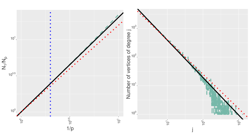
Figure 1: On the left: the plot represent the value of $N_{1}(G_{t})/N_{p}(G_{t})$ as a function of $p$ on a log-log scale. Here $G_{t}$ is a sample from the GGP model of [13] with parameters $(\sigma,\tau)=(0.2,5)$ and $t=2000$ (see also example 5). The sample has 26671 vertices and 293923 edges. With these parameters $\mu$ has a tail-index equal to 0.2. The red dotted line is $y=(1+\sigma)x$, which is the expected asymptotic behaviour of $\log\frac{N_{1}(G_{t})}{N_{p}(G_{t})}$ as a function of $-\log p$. The plain black line is $y=(1+\hat{\sigma}_{p})x$, where $\hat{\sigma}_{p}$ is the estimated value of $\sigma$ using $p=0.5$ (represented by the blue dotted vertical line). On the right: the green curve represents the degree distribution of the same sample. In plain black (respectively dotted red) is represented $\mathsf{d}_{j}\propto j^{-1-\hat{\sigma}_{p}}$ (respectively $\mathsf{d}_{j}\propto j^{-1-\sigma}$ to illustrate that the degree distribution is also governed by the tail-index.

4.2 An estimator and its risk

In view of the heuristic of the previous section, we can construct a simple estimator for $\sigma$. For a chosen value of $p\in(0,1)$, we propose to use as an estimator for $\sigma$,

$$\hat{\sigma}_{p}(G_{t})\coloneqq\begin{cases}\frac{\log N_{1}(G_{t})-\log N_{p}(G_{t})}{-\log p}-1&\mathrm{if}\ N_{p}(G_{t})\geq 1,\\ 0&\mathrm{otherwise}.\end{cases}$$ (4.4)

Notice that $\hat{\sigma}_{p}$ is well-defined since $N_{1}\geq N_{p}$ almost-surely for all $0\leq p\leq 1$. Also note that $\hat{\sigma}_{p}$ does not depend explicitly on the sample size $t$; this is important because $t$ is generally considered to be unknown.

In order to be able to compute the risk of $\hat{\sigma}_{p}$, we require further assumptions on the model. Our first assumption is analogous to the assumptions encountered in [52, 14]. We first introduce the $2$-points correlation function $\nu:\mathbb{R}_{+}^{2}\rightarrow\mathbb{R}_{+}$,

$$\nu(x,x^{\prime})\coloneqq\int_{\mathbb{R}_{+}}W(x,y)W(y,x^{\prime})\,\mathrm{d}y.$$ (4.5)

We also make the following assumption on $\nu$, which is a classical assumption in the literature [52, 14] to be able to control the variance of certain (non-linear) functionals of graphex processes, such has the number of vertices.

Assumption 2.

If $0\leq\sigma<1$, we assume that there is a constant $\eta>\max(1/2,\sigma)$ and a constant $C\geq 0$ such that $\nu(x,x^{\prime})\leq C\mu(x)^{\eta}\mu(x^{\prime})^{\eta}$ for all $x,x^{\prime}\in\mathcal{X}$. If $\sigma=1$, we assume $\nu(x,x^{\prime})\leq C\mu(x)\mu(x^{\prime})$, and we set $\eta=1$.

Also, it is well-known [25, 14], that under equation 3.2 the asymptotic equivalence

$$\int_{\mathbb{R}_{+}}\left(1-e^{-t\mu(z)}\right)\,\mathrm{d}z\sim\begin{cases}t^{\sigma}\ell(t)\Gamma(1-\sigma)&\mathrm{if}\ 0\leq\sigma<1,\\ t\int_{t}^{\infty}z^{-1}\ell(z)\,\mathrm{d}z&\mathrm{if}\ \sigma=1\end{cases}$$ (4.6)

holds as $t\rightarrow\infty$. This relation is already enough to show consistency of $\hat{\sigma}_{p}$. However, further assumptions on $\mu$ are required to bound the bias of the estimator. In the present paper, we shall assume the following.

Assumption 3.

We assume that equation 3.2 holds. We furthermore assume that for all $p\in(0,1)$ there is a sequence $(\Gamma_{p,t})_{t>0}$ such that

$$\left|\frac{\int_{\mathbb{R}_{+}}\left(1-e^{-pt\mu(z)}\right)\,\mathrm{d}z}{p^{\sigma}\int_{\mathbb{R}_{+}}\left(1-e^{-t\mu(z)}\right)\,\mathrm{d}z}-1\right|\leq\Gamma_{p,t}.$$ (4.7)

Assumption 3 is closely related to second-order regular variation assumptions used in extreme values theory [20]. Its purpose is the following. The integral in equation 4.6 plays a determining role in computing the risk of $\hat{\sigma}_{p}$. Equation 4.6, however, says nothing about the rate at which the integral approaches $t^{\sigma}\ell(t)$. Moreover, we know that $\ell(pt)/\ell(t)\rightarrow 1$ as $t\rightarrow\infty$ by the assumptions on $\ell$, but again, the rate of convergence is unknown. These two rates are encapsulated in assumption 3, allowing us to quantify the risk of $\hat{\sigma}_{p}$. Bounds on $\Gamma_{p,t}$ for various examples are given in section 4.3. These examples show that in many cases $\Gamma_{p,t}$ has polynomial decay.

We are now in position to state the main theorem of this section, whose proof is deferred to appendix A.

Theorem 1.

Under assumption 2 and 3, there is a constant $C^{\prime\prime}>0$ depending only on $p$ and $W$ such that for all $t\geq 1$ it holds

$$\mathbb{E}_{W}[(\hat{\sigma}_{p}(G_{t})-\sigma)^{2}]\leq\frac{\Gamma_{p,t}^{2}}{(-\log p)^{2}}+C^{\prime\prime}\log(t)^{2}\max\Big{\{}\frac{1}{t^{1+\sigma}\ell(t)},\,t^{1-2\eta}\Big{\}}.$$ (4.8)

Remark 2.

The computation of the estimator requires to choose a value for $p$. Theoretical guidelines are that any value of $p$ bounded away from zero yields a consistent estimator. But, this leaves unclear how to choose in practice. Optimally, we could build a selection procedure that selects the “optimal” value of $p$, in the sense that bias and variance are suitably balanced. This would however require to make finer assumptions on the structure of the bias. We believe the gain would be marginal as in many cases the value of $\hat{\sigma}_{p}$ is relatively robust to the choice of $p$, see figs. 1 and 4. In practice, we recommend to do a Hill plot to assess the pertinence of estimating $\sigma$ and to determine a reasonable value of $p$, as detailed in section 6.1.

4.3 Discussion about the bias

In [14], the authors suggest to estimate the tail-index using

$$\hat{\sigma}_{\mathrm{CPR}}\coloneqq\frac{2\log\mathsf{v}(G_{t})}{\log\mathsf{e}(G_{t})}-1.$$ (4.9)

It is easily seen that $\mathbb{E}_{W}[(\hat{\sigma}_{\mathrm{CPR}}-\sigma)^{2}]$ is in general a $O(1/\log t)$. Although the variance of $\hat{\sigma}_{p}$ has polynomial decay in $t$, the bias is proportional to $\Gamma_{p,t}$, whose decay can be anything. Hence it is not clear if $\hat{\sigma}_{p}$ dominates $\hat{\sigma}_{\mathrm{CPR}}$ asymptotically. Here we present some examples where the bias of $\hat{\sigma}_{p}$ has also polynomial decay in $t$. We consider the examples which were originally given in [14], because they cover a large spectrum of behaviours.

Example 1.

Dense graphs. Consider the function $W(x,y)=(1-x)(1-y)\mathbf{1}_{x\leq 1}\mathbf{1}_{y\leq 1}$. Then $\mu(x)=0.5(1-x)\mathbf{1}_{x\leq 1}$ and the graph is almost-surely dense. Assumption 2 is trivially satisfied with $\eta=1$. Also, it follows from section C.1 that assumption 3 is satisfied with $\Gamma_{p,t}\propto t^{-1}$: the risk is polynomially decreasing on this example.

Example 2.

Sparse, almost dense graphs without power law. Consider the function $W(x,y)=\exp(-x-y)$. Then $\mu(x)=\exp(-x)$ and assumption 2 is trivially satisfied with $\eta=1$ and $\sigma=0$. Moreover, it follows from section C.2 that assumption 3 is satisfied with $\Gamma_{p,t}\propto 1/\log(t)$: the risk is logarithmically decreasing on this example.

Example 3.

Sparse graphs with power law, separable. For $0<\sigma<1$, consider the function $W(x,y)=(1+x)^{-1/\sigma}(1+y)^{-1/\sigma}$. Then obviously $\mu(x)=\sigma(1+x)^{-1/\sigma}/(1-\sigma)$ and assumption 2 holds trivially with $\eta=1$. Moreover, from section C.3, assumption 3 holds with $\Gamma_{p,t}\propto t^{-\sigma}$: the risk is polynomially decreasing on this example.

Example 4.

Sparse graphs with power law, non separable. For $0<\sigma<1$, consider the function $W(x,y)=(1+x+y)^{-1/\sigma-1}$. It is shown in [14] that assumption 2 holds with $\eta=(1+\sigma)/2$. We have $\mu(x)=\sigma(1+x)^{-1/\sigma}$, which is up to a constant the same marginal as the previous example, so that assumption 3 is verified with $\Gamma_{p,t}\propto t^{-\sigma}$: the risk is polynomially decreasing on this example.

Example 5.

GGP model. For $0\leq\sigma<1$, let $\rho_{\sigma,\tau}(\mathrm{d}x)=\frac{x^{-1-\sigma}\exp(-x)\mathrm{d}x}{\Gamma(1-\sigma)}$, $\bar{\rho}_{\sigma,\tau}(x)\coloneqq\int_{x}^{\infty}\rho_{\sigma,\tau}(\mathrm{d}x)$, and $W(x,y)=1-\exp(-2\bar{\rho}_{\sigma,\tau}^{-1}(x)\bar{\rho}_{\sigma,\tau}^{-1}(y))$. This corresponds to the model in [13]. It is shown in [14] that assumption 2 holds with $\eta=1$. We establish in section C.4 that assumption 3 is satisfied with $\Gamma_{p,t}\propto t^{-\sigma}$: the risk is polynomially decreasing on this example.

Although the asymptotic behaviour of the graphs are relatively close for examples 1 and 2, the bias decay is radically different and estimation is harder in the second example. We also estimated $\mathbb{E}[(\hat{\sigma}_{0.5}-\sigma)^{2}]^{1/2}$ and $\mathbb{E}[(\hat{\sigma}_{0.5}-\sigma)^{2}]^{1/2}$ on the previous examples using $10000$ Monte Carlo samples. In the simulations, we picked $\sigma=0.3$ for the sparse separable and sparse non-separable example, while the GGP example corresponds to a choice of $\sigma=0.5$. The raw numbers are given in tables 1 and 2.

Table 1: Estimation of $\mathbb{E}[(\hat{\sigma}_{0.5}-\sigma)^{2}]^{1/2}$ using 10 000 MC samples for the examples described in section 4.3 and various values of $t$.

$t$	25	50	100	200	400	800
Dense	0.1620	0.0698	0.0327	0.0150	0.0079	0.0039
Almost-dense	0.2971	0.2440	0.2081	0.1814	0.1608	0.1443
Sparse sep. ($\sigma=0.3$)	0.2440	0.1658	0.1186	0.0875	0.0654	0.0488
Sparse non-sep. ($\sigma=0.3$)	0.2947	0.1945	0.1356	0.0966	0.0686	0.0462
GGP ($\sigma=0.5$)	0.1219	0.0801	0.0502	0.0283	0.0110	0.0050

Table 2: Estimation of $\mathbb{E}[(\hat{\sigma}_{\mathrm{CPR}}-\sigma)^{2}]^{1/2}$ using 10 000 MC samples for the examples described in section 4.3 and various values of $t$.

$t$	25	50	100	200	400	800
Dense	0.2719	0.2125	0.1757	0.1500	0.1305	0.1154
Almost-dense	0.4240	0.3882	0.3590	0.3349	0.3144	0.2967
Sparse sep. ($\sigma=0.3$)	0.2963	0.2535	0.2230	0.1994	0.1802	0.1643
Sparse non-sep. ($\sigma=0.3$)	0.3483	0.2947	0.2575	0.2285	0.2051	0.1851
GGP ($\sigma=0.5$)	0.1805	0.1577	0.1392	0.1239	0.1103	0.0982

We pictured in fig. 2 the risk of $\hat{\sigma}_{0.5}$ and $\hat{\sigma}_{\mathrm{CPR}}$ as functions of $t$ for all the simulated examples. As expected, the risk of $\hat{\sigma}_{0.5}$ has polynomial decay every-time but the almost dense example, while the risk of $\hat{\sigma}_{\mathrm{CPR}}$ remains logarithmically decreasing on all examples. We note, however, that even in the situation when the risk has logarithm decay, $\hat{\sigma}_{0.5}$ seems to perform slightly better than $\hat{\sigma}_{\mathrm{CPR}}$.

Figure 2: Comparative plot of $\mathbb{E}[(\hat{\sigma}_{0.5}-\sigma)^{2}]^{1/2}$ against $\mathbb{E}[(\hat{\sigma}_{\mathrm{CPR}}-\sigma)^{2}]^{1/2}$ using 10 000 MC samples for the examples described in section 4.3.

4.4 On the controversy about scale-free nature of real graphs

There is no actual consensus on the scale-free nature of empirical graphs. Here, we briefly review both sides of the debate. This is also an opportunity for us to review what $\sigma$ is and what it isn’t.

According to the general opinion, a finite graph $G$ is called scale-free if there are $c>0$, $\gamma>1$ such that for $j$ large enough

$$\frac{\mathsf{d}_{j}(G)}{\mathsf{v}(G)}\approx cj^{-\gamma}.$$ (4.10)

We left the previous definition intentionally non-rigorous to emphasize one of the origin of the controversy: the lack of consensus on the definition of scale-freeness [30, 54].

Barabási and Albert [4] found that for three empirical networks equation 4.10 seemed true, and they attributed this property to a growth mechanism they called preferential attachment. Since then, many papers claimed to have discovered new types of power-law networks and new mechanism creating them, see for instance [44, 30]. But not everybody agrees, and some authors believe that power-law degree distribution is rarely encountered in practice [32, 16]. The heated debate has culminated recently with [10], claiming that scale-free networks are rare after reviewing a large collection of empirical networks.

The methodology in [10] consists on testing as a null hypothesis a power-law model for the degree distribution against an alternative which is not power-law. On a corpus of 927 empirical networks, which they claim is representative of real networks, they found that only a very few failed to reject the null hypothesis.

Since its first appearance as a preprint [10] has generated a lot of activity, whether it be in agreement or disagreement. We share the same opinion as [30, 54] that the source of the debate is the lack of a rigorous definition. [54] makes an effort toward a clean definition and they arrive at the opposite conclusion of [10]. Another argument against [10], which seems to be the most widespread, is that scale-freeness is only well-defined in the infinite-size limit [30]. According to this view, a network is scale-free if its degree distribution approaches a power-law as the network keeps growing following the same mechanisms. In other word, instead of equation 4.10, we shall say that $\{G_{t}\nonscript\,:\nonscript\,\mathopen{}\allowbreak t\geq 0\}$ is scale-free if

$$\lim_{j\to\infty}\lim_{t\to\infty}\frac{j^{\gamma}\mathsf{d}_{j}(G_{t})}{\mathsf{v}(G_{t})}=c.$$ (4.11)

Then, $\gamma$ is not defined as property of the sample $G_{t}$, but rather as a joint property of the limiting graph and the growth mechanism, equivalently of the sampling design. Here we insist on the importance of the sampling design in the definition: if $\{G_{t}\nonscript\,:\nonscript\,\mathopen{}\allowbreak t\geq 0\}$ is a graphex process, then $\gamma=1+\sigma$ almost-surely under mild conditions [14], though the degree distribution of $G_{t}$ at finite $t$ might have a different index, as illustrated in fig. 3. Another famous example is the traceroute sampling which is known to produce samples with power-law degree distributions, even when the population is not power-law [37, 1]. Another example of this type is provided in section 6.3. Hence, if one is ready to accept equation 4.11 as a definition, talking about scale-freeness without knowledge of the sampling design is irrelevant.

One of the criticism of the definition in equation 4.11 is made on the basis that we never observe $\{G_{t}\nonscript\,:\nonscript\,\mathopen{}\allowbreak t\geq 0\}$ but only $G_{t}$, and that we need tools adapted to finite networks. We have mixed feelings about this. On one hand, the same criticism could be made about any statistical analysis. Indeed, one of the primary goal of statistics is to infer stuff about a population given a sample. In the case of i.i.d observations, we have accepted for a while to idealize the population as an abstract propability distribution, and this has been proven to be very effective in summarizing properties of the population as parameters of the distribution. When the observation is a graph, we have no reason to proceed differently (see in particular in [30] the example of epidemic threshold). On the other hand [30] points out the difficulty in determining the right sampling mechanism, and it is true that models of random networks are commonly misspecified. Then, it is less clear that the parameters make sense, albeit this depends on the degree of misspecification and the task to achieve.

Finally, we note that the test in [10] only involves the degree distribution, but graphs are more than just their degree distribution (see in particular section 6.2.2). For these reason, we don’t believe in the existence of a universal model that can explain all empirical graphs, and it is the work of the statistician to determine a good model for a given task; whence it is useful to study as many models as possible. This opinion seems to be shared by the authors of [10]. We add that in many cases the focus should be put on achieving the task at hand with accuracy rather than trying to explain all the structure of the sample. Besides, the assertion that graphex processes are not desirable to model empirical graphs because power-law graphs are rare is too simplistic: (i) no serious methodology can objectively prove this rarity (what is a representative set of empirical graphs? what definition of scale-freeness to use?), (ii) it is the degree distribution of graphex processes in the infinite size limit which is power-law, and (iii) there are empirical graphs for which some graphex processes have been found to explain well the degree distribution (see [13, 51] and also section 6). Overall, one should not forget to look at other aspects of the modeling that might be more important than just the degree distribution.

4.5 Relation to Hill estimator

Regardless of the controversy of section 4.4, tail-index of the degree distribution of $G_{t}$ is often reported as an interesting summarizing statistics [35, Section 4]. [54] plea in favor of using various estimators as the index is notoriously hard to estimate and different estimators may give very different answers on a given sample. In our opinion, the interest in the tail-index of $G_{t}$ is debatable as it might be unrelated with the index of the population, an issue we already discussed in section 4.4, and which we will emphasize here. The most common reported value for the tail-index of the sample is based on the Hill estimator

$$\hat{\gamma}_{\mathrm{Hill}}(G_{t})\coloneqq\frac{\sum_{j=d_{\min+1}}^{\infty}\mathsf{d}_{j}(G_{t})\log\frac{j}{d_{\min}}}{\sum_{j=d_{\min}+1}^{\infty}\mathsf{d}_{j}(G_{t})},$$ (4.12)

where $d_{\min}>0$ is a cutoff determining where the tail of the degree distribution starts. Most of empirical graphs are reported to have $\hat{\gamma}_{\mathrm{Hill}}\in[2,3]$, while graphex processes have almost-surely index $\gamma=1+\sigma\in[1,2]$, at least if we rely on the definition of equation 4.11. So one might think graphex processes are unrealistic to model graphs with $\hat{\gamma}_{\mathrm{Hill}}\in[2,3]$. Once again, we have to be careful: it is not obvious that the Hill estimator gives consistent answers for $\gamma$. Though it is known from [55] that it is consistent in the preferential attachment model, nothing is known about graphex processes. In particular, in fig. 3 we illustrate what can go wrong: on a simulated sample with true $\sigma=0.3$ (hence $\gamma=1.3$), our estimator gives $\hat{\sigma}_{0.5}=0.3335$, while a non carefully calibrated Hill estimator gives $\hat{\gamma}_{\mathrm{Hill}}=2.1181\in[2,3]$. Once again, this shows that one has to be careful when relating degree distribution of the sample and the idealized degree distribution of the population, i.e. the sampling design has to be taken into account when inferring properties about the population.

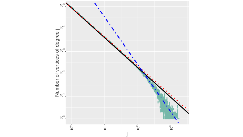
Figure 3: In green is the degree distribution $G_{t}$ is a sample from the GGP model of [13] with parameters $(\sigma,\tau)=(0.3,10)$ and $t=10000$ (see also example 5). The sample has 306791 vertices and 3947805 edges. The red line represents the $\mathsf{d}_{j}\propto j^{-1-\sigma}$. The black line is $\mathsf{d}_{j}\propto j^{-1-\hat{\sigma}_{p}}$, where $\hat{\sigma}_{p}=0.333474$ is computed using $p=0.75$. Finally the blue line is $\mathsf{d}_{j}\propto j^{-\hat{\gamma}_{\mathrm{Hill}}}$, where $\hat{\gamma}_{\mathrm{Hill}}=2.1181$ is computed using $d_{\min}=300$.

5 Count statistics of graphex processes: definition, inference, and hypothesis testing

We briefly discuss how the $p$-sampling argument may also be used to estimate other functionals of $W$. This essentially extends the work of [7, 5] from graphon to graphex. In particular, using $p$-sampling allows to derive a natural notion of bootstrap for networks. Using bootstrap samples, we can then estimate the count statistics of the graph (sections 5.1 and 5.2), which can in turn be used to do nonparametric inference on the (rescaled injective) homomorphism densities (section 5.3). We also use count statistics to construct tests for the number of occurrence of certain motifs (section 5.4). Finally, we discuss the relation of these results with some other works (section 5.5).

5.1 Count statistics

Count statistics have received a lot of attention in the last few years, for multiple reasons. A first reason is that some motifs are of interest to get insights on structure of the network. For instance, counting the number of triangles permit to determine the transitivity of the graph, which is a popular measure of the tendency of the vertices to cluster together [56]. Another reason is that counts of motifs characterize the distribution of the network (see [21] and section 5.3), so that nonparametric inference on the distribution of the network is possible using counts of certain motifs [6, 7, 5]. Other related uses of motifs counts involve hypothesis testing [5] and networks comparison [5, 2].

Count of motifs is notoriously hard, especially when the graph is large and the motif has a large number of vertices. Even counting simple motifs such has triangles might rapidly become intractable on large graphs [48]. Methods based on subsampling the graph have emerged to bypass the complexity. A non exhaustive list of existing methods includes methods based on vertex sampling [5, 34, 2, 41], the parametric bootstrap [28, 39], or based on edge sampling [3, 23, 26, 27]. Here, we take advantage of the $p$-sampling to count motifs. We discuss in section 5.5 how that relates to already existing works, and some of the advantages in doing $p$-sampling over other sampling design.

Before going further, we shall first clarify what me mean by count statistics. For a finite graph $R$, we define the number of copies of $R$ in $G$ as the number of injections $\phi:V(R)\to V(G)$ such that if $\{r_{1},r_{2}\}\in E(R)$ then $\{\phi(r_{1}),\phi(r_{2})\}\in E(G)$, i.e. the number of adjacency preserving map from $R$ to $G$. We call this number $\mathsf{n}(R,G)$, the count statistic of $R$. If $\phi:A\to V(G)$ is injective, we let $G[\phi]$ denote the graph such that $V(G[\phi])=A$ and $\{v,v^{\prime}\}\in E(G[\phi])$ if and only if $\{\phi(v),\phi(v^{\prime})\}\in E(G)$. That is, $G[\phi]$ is isomorphic to the subgraph of $G$ induced by $\phi$. Letting $\mathcal{A}(R,G)$ denote the set of all injections from $V(R)$ to $V(G)$, we can rewrite

$$\mathsf{n}(R,G)=\sum_{\phi\in\mathcal{A}(R,G)}\mathbf{1}\{R\subseteq G[\phi]\}.$$ (5.1)

5.2 Bootstrap estimators for count statistics: model-free results

We first show how to derive a bootstrap estimate for $\mathsf{n}(R,G)$ using $p$-sampling which works for any graph $G$ (so $G$ is not necessarily a graphex process). The result is of interest by itself, since it proves a consistent estimator for $\mathsf{n}(R,G)$ regardless of the distribution of $G$, and that estimator is parallelizable, in contrast with the computation of $\mathsf{n}(R,G)$ which may be challenging for complex motifs $R$. Our estimator is based on the following easy proposition.

Proposition 1.

Let $G\in\mathcal{U}$ and let $R\in\mathcal{L}_{k}$ be a connected graph such that $\mathsf{n}(R,G)<\infty$. Then,

$$\mathbb{E}[\mathsf{n}(R,\mathsf{ps}(G,p))\mid G]=p^{k}\cdot\mathsf{n}(R,G).$$ (5.2)

From the previous proposition, we can obtain a natural estimator of $\mathsf{n}(R,G)$, which we refer as the bootstrap estimator. Indeed, for a fixed $p\in(0,1)$ to be chosen, and for some integer $B\geq 1$, we let $\hat{G}_{1},\dots,\hat{G}_{B}$ be i.i.d copies of $\mathsf{ps}(G,p)\mid G$, and we estimate $\mathsf{n}(R,G)$ by

$$\hat{\mathsf{n}}(R,G)\coloneqq\frac{1}{Bp^{k}}\sum_{b=1}^{B}\mathsf{n}(R,\hat{G}_{b}).$$ (5.3)

The main advantage is that $\mathsf{n}(R,\hat{G}_{b})$ are intrinsically faster to compute than $\mathsf{n}(R,G)$, especially when $G$ is sparse, and computations can be run in parallel. Interestingly, the formula (5.2) is model-free, in the sense that it is true for any graph $G$ that has no isolated vertices. It follows that if $G$ has no isolated vertices, then $\hat{\mathsf{n}}(R,G)$ is an unbiased estimator of $\mathsf{n}(R,G)$, comparable to the Horvitz-Thompson estimator constructed in [34]. The next proposition quantify the risk of $\hat{\mathsf{n}}(R,G)$ as an estimator of $\mathsf{n}(R,G)$.

Proposition 2.

Let $G\in\mathcal{U}$ and let $R\in\mathcal{L}_{k}$ be a connected graph such that $\mathsf{n}(R,G)<\infty$. Then $\hat{\mathsf{n}}(R,G)$ is an unbiased estimator of $\mathsf{n}(R,G)$, and

$$\mathrm{var}(\hat{\mathsf{n}}(R,G)\mid G)=\frac{\mathrm{var}(\mathsf{n}(R,\mathsf{ps}(G,p))\mid G)}{Bp^{2k}}\leq\frac{k}{Bp}\cdot\mathsf{n}(R,G)^{2}.$$ (5.4)

It is worth pointing out that by the previous, $\hat{\mathsf{n}}(R,G)$ is a consistent estimator of $\mathsf{n}(R,G)$ as $B\to\infty$, and thus with almost no condition on $G$. This result is of interest by itself, if one is only interested in counting motifs in $G$ (see also section 6.2).

Remark 3.

In contrast with our estimator for the tail-index, we keep the extra randomness induced by the bootstrap samples, i.e. we have a randomized estimator. But, it is clear from proposition 4 that taking the expectation of $\hat{\mathsf{n}}(R,G)$ conditional on $G$ is pointless. Moreover, the advantage of keeping the randomized-estimator is firstly to enable tractable computations as bootstrap samples can be made arbitrary small.

5.3 Nonparametric inference

Beyond their interest in describing the structure of the network, count statistics permit to estimate the rescaled injective homomorphism densities [8]. Those are distinguished functionals of $W$ whose collection entirely determine $W$ [21, 40, 8]. The rescaled injective homomorphism density of $R$ in $W$ is defined as

$$h(R,W) \coloneqq\frac{\int_{\mathbb{R}_{+}^{\mathsf{v}(R)}}\prod_{\{\ell,m\}\in E(R)}W(x_{\ell},x_{m})\,\mathrm{d}x_{1}\dots\mathrm{d}x_{\mathsf{v}(R)}}{\{\int_{\mathbb{R}_{+}^{2}}W(x_{1},x_{2})\,\mathrm{d}x_{1}\mathrm{d}x_{2}\}^{\mathsf{v}(R)/2}}.$$ (5.5)

It follows from [21, 40, 8] that $W$ can be in principle recovered – up to measure preserving transformations – from the collection of all $\{h(R,W)\nonscript\,:\nonscript\,\mathopen{}\allowbreak R\in\mathcal{L}\}$. We shall only consider motifs $R$ and processes for which the previous quantity is finite. Indeed, we will assume that a certain number of moments of $W$ are finite.

Assumption 4.

A graphex process $\{G_{t}\nonscript\,:\nonscript\,\mathopen{}\allowbreak t\geq 0\}$ with graphon function $W:\mathbb{R}_{+}^{2}\to[0,1]$ satisfies this assumption for $N\geq 1$ integer if,

$$\max_{n=1,\dots,N}\max_{\begin{subarray}{c}R\in\mathcal{L}_{n}\\ R\,\mathrm{connected}\end{subarray}}\int_{\mathbb{R}_{+}^{n}}\prod_{\{\ell,m\}\in E(R)}W(x_{\ell},x_{m})\,\mathrm{d}x_{1}\dots\mathrm{d}x_{n}<\infty.$$ (5.6)

Then, we have the following result, borrowed from [8, Proposition 56].

Proposition 3.

Let $R\in\mathcal{L}_{k}$ be a connected graph. If $\{G_{t}\nonscript\,:\nonscript\,\mathopen{}\allowbreak t\geq 0\}$ is a graphex process satisfying assumption 4 with $N=k$, then almost-surely,

$$\lim_{t\to\infty}t^{-k}\mathsf{n}(R,G_{t})=\int_{\mathbb{R}_{+}^{k}}\prod_{\{\ell,m\}\in E(R)}W(x_{\ell},x_{m})\,\mathrm{d}x_{1}\dots\mathrm{d}x_{k}.$$ (5.7)

The consequence of the last proposition is that $h(R,W)$ can be consistently estimated as $t\to\infty$ by

$$\hat{h}(R,G_{t})\coloneqq\frac{\mathsf{n}(R,G_{t})}{\mathsf{e}(G_{t})^{\mathsf{v}(R)/2}},$$ (5.8)

where in turn we can leverage the consistency of our bootstrap estimator of $\mathsf{n}(R,G_{t})$ to make computations tractable. We note that the method of moments of [7] can be adapted to estimate $W$ from $\hat{h}(R_{1},G_{t}),\hat{h}(R_{2},G_{t}),\dots$ for clever choice of motifs $R_{1},R_{2},\dots$.

5.4 Hypothesis testing

Besides their interest for estimating $W$, the count statistics have been used in testing equality of features of networks and finding confidence intervals of the count feature [42, 47]. The authors of [5] have an example where they use counts of certain motifs to test if the dearth of short-cycles in a network is statistically significant. As argued in [5], the main challenge is then the problem of finding estimates of $s_{t}^{2}(R)\coloneqq\mathrm{var}_{W}(\mathsf{n}(R,G_{t}))$. Here we show how the $p$-sample argument can be used in order to recycle the bootstrap samples to estimate $s_{t}^{2}(R)$, which provides a somewhat simpler estimator than in [5]. Our estimator is based on the result of the following proposition.

Proposition 4.

Let $\{G_{t}\nonscript\,:\nonscript\,\mathopen{}\allowbreak t\geq 0\}$ be a graphex process satisfying assumption 4 with $N=2k-1$. For any connected graph $R\in\mathcal{L}_{k}$, as $t\to\infty$

$$s_{t}^{2}(R) =\frac{\mathbb{E}_{W}[\mathrm{var}(\mathsf{n}(R,\mathsf{ps}(G_{t},p))\mid G_{t})]}{p^{2k-1}(1-p)}+O(t^{2k-2}).$$ (5.9)

This suggests that $s_{t}^{2}(R)$ may be estimated by

$$\hat{s}^{2}(R,G_{t})\coloneqq\frac{\mathrm{var}(\mathsf{n}(R,\mathsf{ps}(G_{t},p))\mid G_{t})}{p^{2k-1}(1-p)},$$ (5.10)

where in turn the variance in the numerator of the last display can be approximated up to arbitrary precision by recycling the bootstrap samples used for the estimation of $\mathsf{n}(R,G_{t})$. The next proposition establishes that $\hat{s}^{2}(R)$ is consistent.

Proposition 5.

Let $\{G_{t}\nonscript\,:\nonscript\,\mathopen{}\allowbreak t\geq 0\}$ be a graphex process satisfying assumption 4 with $N=4k-2$. For any connected graphs $R\in\mathcal{L}_{k}$, as $t\to\infty$

$$\frac{\hat{s}^{2}(R,G_{t})}{s_{t}^{2}(R)}=1+O_{p}(t^{-1/2}).$$ (5.11)

The fact that we are able to consistently estimate $s_{t}^{2}(R)$ permit to perform hypothesis testing for $\bar{\mathsf{n}}(R,W,t)\coloneqq\mathbb{E}_{W}[\mathsf{n}(R,G_{t})]$. In particular, it is of interest to construct tests for $H_{0}:\bar{\mathsf{n}}(R,W,t)=\bar{\mathsf{n}}(R,W_{0},t_{0})$ against $H_{a}:\bar{\mathsf{n}}(R,W,t)\neq\bar{\mathsf{n}}(R,W_{0},t_{0})$, see for instance section 6.2.2 and also [5]. We show in the next proposition that asymptotically consistent testing for these hypotheses can be made on the basis of the test statistic

$$T(R,G_{t}) \coloneqq\frac{\mathsf{n}(R,G_{t})-\bar{\mathsf{n}}(R,W_{0},t_{0})}{\sqrt{\hat{s}^{2}(R,G_{t})}}.$$ (5.12)

Proposition 6.

Let $\{G_{t}\nonscript\,:\nonscript\,\mathopen{}\allowbreak t\geq 0\}$ be a graphex process with graphon function $W_{0}$ satisfying assumption 4 with $N=4k$. For any connected graphs $R\in\mathcal{L}_{k}$, $T(R,G_{t_{0}})\xrightarrow{d}\mathcal{N}(0,1)$ as $t_{0}\to\infty$.

Remark 4.

It would also be of interest to construct a test for the weaker hypothesis $H_{0}:h(R,W)=h(R,W_{0})$. It seems to us that this is a much harder problem. Indeed, it is true that $\hat{h}(R,G_{t})\sim h(R,W_{0})$ almost-surely under $H_{0}$ by [8], and so we could imagine constructing a test based on $\hat{h}$. However, the statistical fluctuations of $\mathsf{n}(R,G_{t})-\mathbb{E}_{W}[\mathsf{n}(R,G_{t})]$ and of $\mathsf{e}(G_{t})-\mathbb{E}_{W}[\mathsf{e}(G_{t})]$ are exactly of the same order, which makes the asymptotic normality of $\hat{h}(R,G_{t})$ less evident.

5.5 Relation to other works

The work presented here relates to many of the paper cited previously. In our opinion, the two most related papers are the work of [5] and of [34]. We now discuss the relation between these papers and our results.

In [5], the authors consider nonparametric estimation of certain functionals of the graphon in a sparse graphon model, with applications in hypotheses testing and networks comparison. The sparse graphon model and the graphex model are different, though they are tightly related, as explained for instance in [8]. The functionals considered in [5, 7] are related to the expectation of counts of motifs too. We note, however, that they use a slightly different notion of counts than $\mathsf{n}(R,G_{t})$, though this do not fundamentally make difference and their procedures can be easily adapted to $\mathsf{n}(R,G_{t})$. The paper [5] consider two subsampling procedures for counting motifs. Of particular interest for us is their uniform subsampling bootstrap. Given a sample $G_{n}$ with $n$ vertices, they consider the subgraph $\tilde{G}_{n,m}$ which consists on uniformly sampling $m<n$ vertices without replacement of $G_{n}$ and returning the induced subgraph. For moderate $m$, this is morally equivalent to $p$-sampling. Sampling vertices without replacement is quite natural for dense graphon sample, but less evident in the case of a sparse graphon sample. The issue is for instance discussed in [41]: in the classical dense graphon model $\tilde{G}_{n,m}\overset{d}{=}G_{m}$, which is not necessarily true in the sparse model. This is not an issue to estimate $\mathsf{n}(R,G_{n})$, but it is if one wants to estimate $\mathrm{var}(\mathsf{n}(R,G_{n}))$, to do hypothesis testing for instance. Because the distribution of $\tilde{G}_{n,m}$ has no distinguished properties, it is unclear that $\mathrm{var}(\mathsf{n}(R,G_{n}))$ can be estimated from $\mathrm{var}(\mathsf{n}(R,\tilde{G}_{n,m})\mid G_{n})$; so [5] have to rely on rather complicated procedures to estimate $\mathrm{var}(\mathsf{s}(R,G_{n}))$.

In [34], the authors are also interested in estimating the counts of certain motifs using vertex sampling. They also consider two subsampling schemes. In particular, they consider uniform subsampling of vertices, which is almost $p$-sampling. The only difference is that they keep isolated vertices in the subsample while we don’t. Since we only consider connected motifs, the two methods are the same, as isolated vertices cannot contribute to the motif. Consequently, our results in section 5.2 are partial restatements of [34], though they also consider a different notion of counts. We note that in [34] the authors are only interested in counting motifs. They don’t make probabilistic assumption on the graph and hence do not consider inference on the distribution of the graph.

6 Some applications

6.1 Assessing the pertinence of sparse graphex models on some real networks

The tail-index of $\mu$ is a distinguished feature of sparse graphex processes (i.e. graphex processes satisfying assumptions 1, 3 and 2 for $\sigma\neq 0$). As such, it can be used to diagnose the pertinence of using such a model on some real datasets. In particular, if $G_{t}$ is a sample of a sparse graphex process, then we expect the degree distribution of $G_{t}$ to be close to a power-law with index $1+\sigma$, and $p\mapsto\log\frac{N_{1}(G_{t})}{N_{p}(G_{t})}$ to be closely linear with slope $1+\sigma$, at least for $p$ bounded away from $0$ (the asymptotic being true only in this region). Equivalently, we might look at the plot of $p\mapsto\hat{\sigma}_{p}(G_{t})$, which we call a Hill plot in analogy with the classical Hill plots used in extreme value theory to calibrate the Hill estimator [22]. If the model is correct, we expect the Hill plot to be constant, except perhaps at the boundary close to $p=0$. The Hill plot is doubly interesting as it allows for both assessing the pertinence of the model, but also to choose a reasonable value of $p$ for the estimation of the tail-index (see also remark 2).

We choose to illustrate the diagnostic on two datasets from [43], the Flickr and the Youtube datasets. These datasets are available from the KONECT database [36]. These are social networks datasets where vertices are users and edges represent friendships. We note that the Flickr dataset is a directed graph, but we ignore arrows and see it as an undirected graph. We summarize in table 3 the main statistics of these networks.

Table 3: Summary of main statistics for the Flickr and Youtube networks.

Network	Number of vertices	Number of edges
Flickr	2302926	22838277
Youtube	3223586	9375375

These two networks are interesting in the way they have been sampled. Indeed, [43] crawled these networks by searching for the whole connected component reachable from a random set of users. The methodology may be summarized as starting from a single user, and in each step, retrieve the list of friends for a not yet visited user and add these users to a list of users to visit. The process is continued until exhaustion of the list. This is known as breadth-first search (BFS) sampling. Interestingly, [43] crawled the Flickr and Youtube networks using BFS sampling every day on a large period of time (several weeks). In particular, each day they revisited all the users they had previously discovered, and in addition all the new users that were reachable from the previously known users. By choosing a reasonable sets of users to start with, they have access to the whole largest connected component of these networks. Further, provided the BFS sampling goes well, their crawling mechanism may be viewed as observing snapshots of a graphex process at increasing times.

We plotted side-by-side the Hill plot and the degree distribution, respectively for the Flickr and Youtube networks, in figs. 4 and 5.

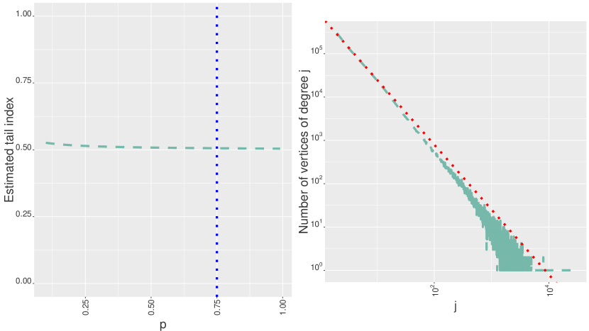
Figure 4: On the left: The Hill plot of $\hat{\sigma}_{p}$ estimated on the Flickr dataset, that is the plot of $p\mapsto\hat{\sigma}_{p}$. The vertical blue line at $p=0.75$ corresponds to the retained value for the estimation of $\sigma$. We notice that the Hill plot is essentially flat in this case, which is the expected behaviour when the model is well-specified. On the right: In green is the degree distribution of the Flickr dataset. In red is the line corresponding to $\mathsf{d}_{j}\propto j^{-1-\hat{\sigma}_{p}}$. We see that both curves align well.

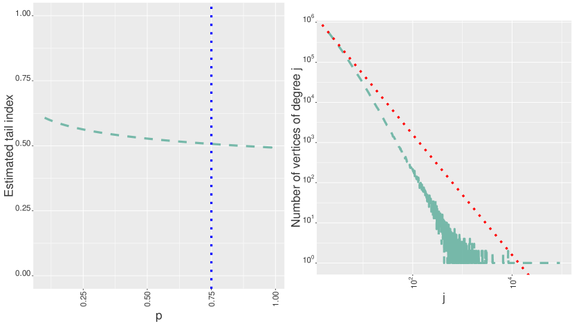
Figure 5: On the left: The Hill plot of $\hat{\sigma}_{p}$ estimated on the Youtube dataset, that is the plot of $p\mapsto\hat{\sigma}_{p}$. The vertical blue line at $p=0.75$ corresponds to the retained value for the estimation of $\sigma$. We notice that the Hill plot is not flat, which should be considered as a warning that the model might be inadequate. On the right: In green is the degree distribution of the Youtube dataset. In red is the line corresponding to $\mathsf{d}_{j}\propto j^{-1-\hat{\sigma}_{p}}$.

We plotted the degree distributions on a log-log scale, and added in red dotted lines a linear curve with slope $-(1+\hat{\sigma}_{p})$, where $\hat{\sigma}_{p}$ has been computed using $p=0.75$. In case the model is correct, we then expect the degree distribution and the linear curve to align well. We can see in fig. 6 that the Flickr dataset exhibits some features of sparse graphex processes: its Hill plot is relatively flat with value $\approx 0.5$, and the slope of its degree distribution on a log-log scale is close to $\approx-1.5$. Regarding the Youtube dataset, in fig. 5, this is less evident, even the plots plea in favor of a misspecification of the sparse graphex model. This might be because the model is not reasonable, which is likely to be caused by the crawling procedure used in [43]: the data they have at their disposal make uncertain that all users in Youtube have effectively been sampled [43, Section 4.2.4].

Finally, we mention that these plots should only be used as visual diagnostics, and it is hard to draw firm conclusions about the validity of the model from these plots. One would need in particular to do a true statistical test for the degree distribution, yet this is unclear how to perform at this time.

6.2 Counting motifs

6.2.1 Consistent estimation of count statistics

We can also use the results of section 5.2 to count the number of motifs in a network. We illustrate this on the number of triangles in the Youtube network of the previous section. We note here that the number of triangles is equal to $\mathsf{n}(R,G_{t})/6$ where $R$ is a triangle graph. We also note that the method is consistent regardless of the distribution of $G_{t}$, whence it does not matter that we found evidence that the Youtube dataset is unlikely to be a sample of a sparse graphex process. We plot in fig. 6 the estimated number of triangles and the estimated standard deviation as a function of the number of bootstrap samples used. The bootstrap samples used are small ($p=0.01$), implying that in average each sample has $\approx 12$ triangles, which is fast to count. Yet, with only 2000 samples (which can all be computed in parallel) the accuracy is already quite good.

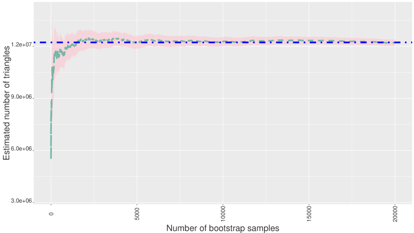
Figure 6: In green is the plot of (one realization of) the estimated number of triangles using $p$-sampling of the Youtube dataset, as a function of the number of bootstrap sample used ($p=0.01$). The horizontal blue line corresponds to the true number of triangles. The pink region is $[\hat{\mathsf{n}}(R,G)\pm 2\delta]$, where $\delta^{2}$ is the empirical estimate of $\mathrm{var}(\hat{\mathsf{n}}(R,G)\mid G)$.

6.2.2 Testing for count statistics

We have seen in section 6.1 that the degree distribution of the Flickr network was plausibly well explained as a sample from a graphex process. In particular it is found that $\sigma=0.5$ does explain quite well the “sparsity” and the degree distribution. The current state if the art algorithm for inference on graphex processes is the algorithm of [13] and its subsequent generalization in [51]. Here we focus on the simpler version of Caron and Fox [13]. Caron and Fox’s algorithm is based on the GGP model previously described in example 5. Hence the model is a parametric family with parameter set $\{W\equiv W_{\sigma,\tau}\nonscript\,:\nonscript\,\mathopen{}\allowbreak\sigma<1,\,\tau>0\}$. One of the desirable feature of the GGP model is that the parameter $\sigma$ is exactly the tail-index of $\mu$ described in section 3.4. Yet simple, this model is able to accommodate for $\sigma\in[0,1)$, that is from dense to sparse with power-law. The other parameter $\tau$ acts as a cut-off for the degree distribution, controlling the separation between the power-law regime and non power-law regime (corresponding to larger degrees), see [13]. In particular, the GGP model with $(\sigma,\tau,t)=(0.5,6.3,12000)$ satisfies $\mathbb{E}_{W}[\mathsf{v}(G_{t})]\approx 2.3$ millions and $\mathbb{E}_{W}[\mathsf{e}(G_{t})]\approx 23$ millions. So, the degree distribution and the size of Flickr are well explained by the GGP model with $(\sigma,\tau,t)=(0.5,6.3,12000)$, as emphasized by tables 3 and 7. Due to its relative simplicity, this model enables for efficient and tractable computations [13, 51]. Then, it makes sense to determine if other aspects of the structure of Flickr can be as well explained by the same model. Here we test if the number of triangles observed in Flickr is compatible with the GGP model with $H_{0}:(\sigma_{0},\tau_{0},t_{0})=(0.5,6.3,12000)$. Under $H_{0}$, by numerical integration we find that $\bar{\mathsf{n}}(R,W_{0},t_{0})=3.75\cdot 10^{8}$ when $R$ is a triangle. Using the bootstrap procedure of section 5 on the Flickr dataset (we used $p=0.1$ and $2000$ bootstrap samples), we estimated $\mathsf{n}(R,G_{t})=5.03\cdot 10^{9}$ and $\sqrt{\hat{s}^{2}(G_{t})}=1.93\cdot 10^{8}$. This gives an observed value of the test statistic $T(R,G_{t})$ of approximately $24.2$, and then a $p$-value $\approx 0$. Hence $H_{0}$ is rejected in this case: without surprise it does not seem reasonable that the Flickr dataset is well-explained by a model as simple as the GGP model. This emphasize the need of more advanced algorithm for inference, in particular for non-parametric estimation.

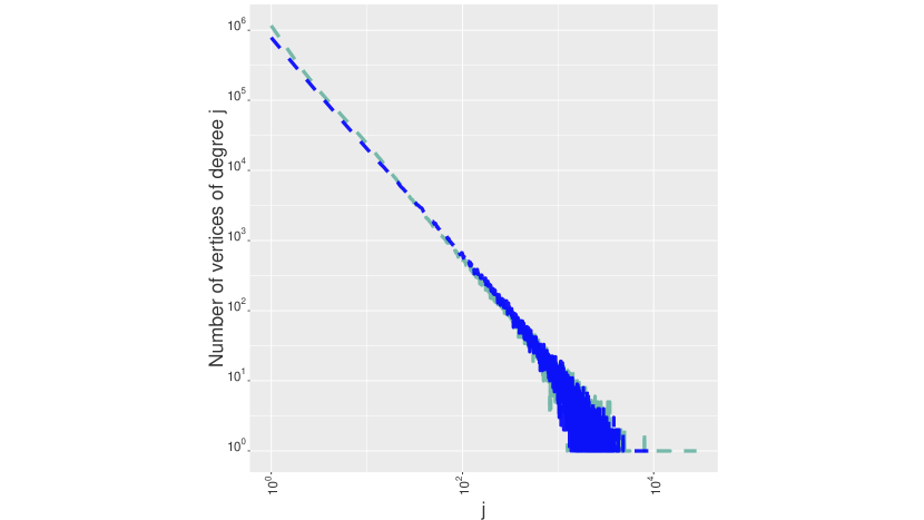
Figure 7: In green is the degree distribution of the Flickr datasat. In blue, the degree distribution of one sample of a GGP model with parameters $(\sigma,\tau,t)=(0.5,6.3,12000)$.

6.3 Test-train split

Model evaluation is a key component of data analysis. Often, this involves randomly splitting the available data into a test set and a training set. There are many seemingly natural ways to partition a graph, so some care is required in splitting the data. The choice of partitioning scheme may induce a significant sampling bias in the test and training sets, impeding evaluation and complicating model comparison. Consider for instance the case of independent and identically distributed observations $(Y_{1},\dots,Y_{n})\overset{iid}{\ \sim\ }P^{n}$: it is natural to split the data $(Y_{1},\dots,Y_{n})$ by subsampling uniformly without replacement $0\leq m\leq n$ observations within the sample. This is because the obtained subsample has the desirable property to be distributed according to $P^{m}$. We argue that in the context of graphex processes, the natural way to split the graph is precisely the $p$-sampling procedure described in section 3.3, because it is the only procedure leaving (up to rescaling) the distribution of the graph invariant [53, 9].

To illustrate the difficulty with test–train splitting of graphs, we built two training sets from the Flickr dataset: one using the $p$-sampling procedure, and the other using the so-called star sampling [11, 35]. The star sampling we used consists on selecting a set of vertices by uniform sampling with probability $p^{\prime}$ (the stars centers), and for each of these center select all of its neighbors (the star points), and then returning the induced subgraph. We used $p=0.2$ and $p^{\prime}=0.013\dots$ to obtain training sets with a comparable number of vertices (respectively 201633 for $p$-sampling and 193075 for star sampling). However, the structure of the obtained training sets are very different. The $p$-sample training set has 952723 edges, while the star sample has 15739418 edges. Whence the star training set is much denser, as expected. The degree distributions of the two training sets are also quite different, as illustrated in fig. 8. On the same figure, we drew a line with slope $-1.5$, which was found to explain well the degree distribution of the complete dataset. We see that it adjusts also quite well the degree distribution of the $p$-sampled training-set. So at least in term of degree distribution, the $p$-sampling training set captures better the structure of the complete dataset.

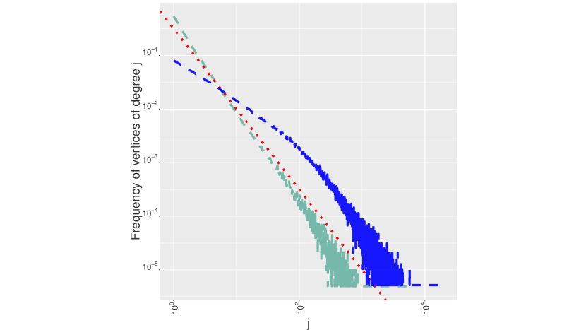
Figure 8: In green: the degree distribution of a $p$-sampling of the Flickr dataset with $p=0.2$ (the sample has 201633 vertices and 952723 edges). In blue: the degree distribution of a star sampling of the Flickr dataset with $p^{\prime}=0.013\dots$ (the sample has 193075 vertices and 15739418 edges). In red is $\mathsf{d}_{j}\propto j^{-1.5}$ which was found to be a credible estimate of the degree distribution of the complete Flickr dataset.

Appendix A Proofs related to tail-index estimation

A.1 Preliminaries

We let $\bm{B}\coloneqq(B_{i,j})_{(i,j)\in\mathbb{N}^{2}}$ be the symmetric array of binary variables that indicate that $v_{i}$ and $v_{j}$ are connected if $B_{i,j}=1$, not connected if $B_{i,j}=0$. All other quantities are defined in the main document. We drop out the subscript $W$ for convenience, and $\mathbb{E}$ shall be interpreted as $\mathbb{E}_{W}$. Also, to simplify notations, we write $N_{1,t}\equiv N_{1}(G_{t})$, $N_{p,t}\equiv N_{p}(G_{t})$, and $\hat{\sigma}_{p,t}\equiv\hat{\sigma}_{p}(G_{t})$.

A.2 Bias-variance decomposition

The starting point of the proof is to decompose the risk onto a deterministic bias term and some stochastic variance terms. Then, when $N_{p,t}=0$ we have

$$(\hat{\sigma}_{p,t}-\sigma)^{2}=\sigma^{2}\leq 1.$$ (A.1)

In the situation where $N_{p,t}\geq 1$, we have

$$-\log(p)\hat{\sigma}_{p,t}=\log\frac{\mathbb{E}N_{1,t}}{\mathbb{E}N_{p,t}}+\log p+\log\left(1+\frac{N_{1,t}-\mathbb{E}N_{1,t}}{\mathbb{E}N_{1,t}}\right)\\ -\log\left(1+\frac{N_{p,t}-\mathbb{E}N_{p,t}}{\mathbb{E}N_{p,t}}\right).$$ (A.2)

To ease notations, we define,

$$b_{\sigma,t}\coloneqq\frac{\log(\mathbb{E}N_{1,t}/\mathbb{E}N_{p,t})}{-\log p}-1-\sigma,\quad Z_{p}\coloneqq\frac{N_{p,t}-\mathbb{E}N_{p,t}}{\mathbb{E}N_{p,t}}.$$ (A.3)

Note that $Z_{1},Z_{p}>-1$ because $N_{1,t}\geq N_{p,t}\geq 1$. Then when $N_{p,t}\geq 1$,

$$(\hat{\sigma}_{p,t}-\sigma)^{2} =\left(b_{\sigma,t}+\frac{\log(1+Z_{1})}{-\log p}-\frac{\log(1+Z_{p})}{-\log p}\right)^{2}$$ (A.4)

$$=b_{\sigma,t}^{2}+2b_{\sigma,t}\frac{\log(1+Z_{1})}{-\log p}-2b_{\sigma,t}\frac{\log(1+Z_{p})}{-\log p}$$ (A.5)

$$\quad+\frac{\log^{2}(1+Z_{1})}{(-\log p)^{2}}+\frac{\log^{2}(1+Z_{p})}{(-\log p)^{2}}-2\frac{\log(1+Z_{1})\log(1+Z_{p})}{(-\log p)^{2}}.$$ (A.6)

We now introduce functions $\varphi_{1},\varphi_{2}:(-1,\infty)\rightarrow\mathbb{R}_{+}$ such that for every $z\neq 0$,

$$\varphi_{1}(z)\coloneqq\frac{\log(1+z)}{z},\qquad\varphi_{2}(z)\coloneqq-\frac{\log(1+z)-z}{z^{2}}.$$ (A.7)

For $z=0$ the functions $\varphi_{1}$ and $\varphi_{2}$ are extended by continuity. The functions $\varphi_{1}$ and $\varphi_{2}$ are non-negative and monotonically decreasing on $(-1,\infty)$. We can therefore write when $N_{p,t}\geq 1$,

$$(\hat{\sigma}_{p,t}-\sigma)^{2}=b_{\sigma,t}^{2}+\frac{Z_{1}^{2}\varphi_{1}(Z_{1})^{2}}{(-\log p)^{2}}+\frac{Z_{p}^{2}\varphi_{1}(Z_{p})^{2}}{(-\log p)^{2}}-2\frac{Z_{1}Z_{p}\varphi_{1}(Z_{1})\varphi_{1}(Z_{p})}{(-\log p)^{2}}\\ +\frac{2b_{\sigma,t}Z_{1}}{-\log p}-\frac{2b_{\sigma,t}Z_{1}^{2}\varphi_{2}(Z_{1})}{-\log p}-\frac{2b_{\sigma,t}Z_{p}}{-\log p}+\frac{2b_{\sigma,t}Z_{p}^{2}\varphi_{2}(Z_{p})}{-\log p}.$$ (A.8)

But, by Young’s inequality we have $2|Z_{1}Z_{p}\varphi_{1}(Z_{1})\varphi_{1}(Z_{p})|\leq Z_{1}^{2}\varphi_{1}(Z_{1})^{2}+Z_{p}^{2}\varphi_{2}(Z_{p})^{2}$. Combining the Young inequality estimate with equations (A.1) and (A.8) gives

$$\mathbb{E}[(\hat{\sigma}_{p,t}-\sigma)^{2}] =\mathbb{E}[(\hat{\sigma}_{p,t}-\sigma)^{2}\mathbf{1}_{N_{p,t}=0}]+\mathbb{E}[(\hat{\sigma}_{p,t}-\sigma)^{2}\mathbf{1}_{N_{p,t}\geq 1}]$$ (A.9)

$$\leq\mathbb{P}(N_{p,t}=0)+b_{\sigma,t}^{2}+\frac{2\mathbb{E}[Z_{1}^{2}\varphi_{1}(Z_{1})^{2}\mathbf{1}_{N_{p,t}\geq 1}]}{(-\log p)^{2}}+\frac{2b_{\sigma,t}\mathbb{E}[Z_{1}\mathbf{1}_{N_{p,t}\geq 1}]}{-\log p}$$ (A.10)

$$\quad+\frac{2\mathbb{E}[Z_{p}^{2}\varphi_{1}(Z_{p})^{2}\mathbf{1}_{N_{p,t}\geq 1}]}{(-\log p)^{2}}-\frac{2b_{\sigma,t}\mathbb{E}[Z_{p}\mathbf{1}_{N_{p,t}\geq 1}]}{-\log p}$$ (A.11)

$$\quad+\frac{2b_{\sigma,t}\mathbb{E}[Z_{p}^{2}\varphi_{2}(Z_{p})\mathbf{1}_{N_{p,t}\geq 1}]}{-\log p}-\frac{2b_{\sigma,t}\mathbb{E}[Z_{1}^{2}\varphi_{2}(Z_{1})\mathbf{1}_{N_{p,t}\geq 1}]}{-\log p}.$$ (A.12)

Moreover, because $\mathbb{E}[Z_{1}]=\mathbb{E}[Z_{p}]=0$ we get by Hölder’s inequality the following estimates.

$$\mathbb{E}[Z_{1}\mathbf{1}_{N_{p,t}\geq 1}]=\mathbb{E}[Z_{1}(1-\mathbf{1}_{N_{p,t}=0})]\leq\mathbb{E}[|Z_{1}|\mathbf{1}_{N_{p,t}=0}]\leq\sqrt{\mathbb{E}[Z_{1}^{2}]\mathbb{P}(N_{p,t}=0)}$$ (A.13)

$$\mathbb{E}[Z_{p}\mathbf{1}_{N_{p,t}\geq 1}]=\mathbb{E}[Z_{p}(1-\mathbf{1}_{N_{p,t}}=0)]=\mathbb{P}(N_{p,t}=0).$$ (A.14)

Also, because $\mathbb{E}[N_{p,t}]>0$ (see proposition 7 below), by Chebychev inequality, for any $t<1$,

$$\mathbb{P}(N_{p,t}=0)\leq\mathbb{P}(N_{p,t}<\mathbb{E}N_{p,t}(1-t))\leq\mathbb{P}(Z_{p}<-t)\leq\frac{\mathbb{E}[Z_{p}^{2}]}{t^{2}}.$$ (A.15)

Since this is true for all $t<1$, we certainly have $\mathbb{P}(N_{p,t}=0)\leq\mathbb{E}[Z_{p}^{2}]$. Furthermore, $N_{1,t}\geq N_{p,t}\geq 1$ implies that $Z_{1}\geq-1+(\mathbb{E}N_{1,t})^{-1}$, then

$$\varphi_{1}(Z_{1})\mathbf{1}_{N_{p,t}\geq 1}\leq\frac{\log\mathbb{E}N_{1,t}}{1-(\mathbb{E}N_{1,t})^{-1}}.$$ (A.16)

Also,

$$\varphi_{2}(Z_{1})=\varphi_{1}(Z_{1})-\frac{(1+Z_{1})\log(1+Z_{1})-Z_{1}}{Z_{1}^{2}}\leq\varphi_{1}(Z_{1}).$$ (A.17)

Obviously, the same estimates hold for $Z_{p}$. Combining all the previous estimates yield the bound (where $(x)_{+}=x$ if $x\geq 0$ and $(x)_{+}=0$ if $x<0$),

$$\mathbb{E}[(\hat{\sigma}_{p,t}-\sigma)^{2}]\leq b_{\sigma,t}^{2}+\left[1+\frac{2(-b_{\sigma,t})_{+}}{-\log p}\right]\mathbb{E}[Z_{p}^{2}]+\frac{2(b_{\sigma,t})_{+}}{-\log p}\sqrt{\mathbb{E}[Z_{1}^{2}]\mathbb{E}[Z_{p}^{2}]}\\ \begin{aligned} &+\left[\frac{\log\mathbb{E}N_{1,t}}{1-(\mathbb{E}N_{1,t})^{-1}}\right]^{2}\frac{2\mathbb{E}[Z_{1}^{2}]}{(-\log p)^{2}}+\left[\frac{\log\mathbb{E}N_{1,t}}{1-(\mathbb{E}N_{1,t})^{-1}}\right]\frac{2(-b_{\sigma,t})_{+}\mathbb{E}[Z_{1}^{2}]}{-\log p}\\ &+\left[\frac{\log\mathbb{E}N_{p,t}}{1-(\mathbb{E}N_{p,t})^{-1}}\right]^{2}\frac{2\mathbb{E}[Z_{p}^{2}]}{(-\log p)^{2}}+\left[\frac{\log\mathbb{E}N_{p,t}}{1-(\mathbb{E}N_{p,t})^{-1}}\right]\frac{2(b_{\sigma,t})_{+}\mathbb{E}[Z_{p}^{2}]}{-\log p}.\end{aligned}$$ (A.18)

Then the conclusion of theorem 1 follows from the estimates in sections A.3 and A.4.

A.3 Study of the bias term $b_{\sigma,t}$

The estimate for the bias term follows from the expectation of $N_{p,t}$ for $p\in[0,1]$ given in the next proposition. Remark that from the definition of $N_{p,t}$, recalling $\mathcal{V}=\{(t_{1},x_{1}),\dots\}$, we have

$$N_{p,t}\overset{d}{=}\begin{cases}p\sum_{i}\mathbf{1}_{t_{i}\leq t}\left(1-(1-p)^{\sum_{j\neq i}B_{i,j}\mathbf{1}_{t_{j}\leq t}}\right)&\mathrm{if}\ 0\leq p<1,\\ \sum_{i}\mathbf{1}_{t_{i}\leq t}\mathbf{1}\{\sum_{j\neq i}B_{i,j}\mathbf{1}_{t_{j}\leq t}>0\}&\mathrm{if}\ p=1.\end{cases}$$ (A.19)

Proposition 7.

For any $p\in[0,1]$ and $t>0$ it holds,

$$\mathbb{E}[N_{p,t}]=pt\int_{\mathbb{R}_{+}}\left(1-e^{-pt\mu(x)}\right)\,\mathrm{d}x.$$ (A.20)

Proof.

We assume here that $p\neq 1$. The case $p=1$ follows from similar steps, or by taking cautiously the limit $p\rightarrow 1$ in the proof. Then we have,

$$\mathbb{E}[N_{p,t}] =p\mathbb{E}\left[\sum_{i}\mathbf{1}_{t_{i}\leq t}\left(1-(1-p)^{\sum_{j\neq i}B_{i,j}\mathbf{1}_{t_{j}\leq t}}\right)\right]$$ (A.21)

$$=p\mathbb{E}\left[\sum_{i}\mathbf{1}_{t_{i}\leq t}\left(1-\mathbb{E}\left[(1-p)^{\sum_{j\neq i}B_{i,j}\mathbf{1}_{t_{j}\leq t}}\mid\mathcal{V}\right]\right)\right]$$ (A.22)

$$=p\mathbb{E}\left[\sum_{i}\mathbf{1}_{t_{i}\leq t}\left(1-\textstyle\prod_{j\neq i}\mathbb{E}\left[(1-p)^{B_{i,j}\mathbf{1}_{t_{j}\leq t}}\mid\mathcal{V}\right]\right)\right],$$ (A.23)

where the last line follows from independence and dominated convergence theorem to take care of the infinite product. It is easily seen from the definition of $\bm{B}$ that for all $i\neq j$,

$$\mathbb{E}[(1-p)^{B_{i,j}\mathbf{1}_{t_{j}\leq t}}\mid\mathcal{V}]=1-pW(x_{i},x_{j})\mathbf{1}_{t_{j}\leq t}.$$ (A.24)

It follows, invoking the Slivnyak-Mecke formula [19, Chapter 13],

$$\mathbb{E}[N_{p,t}] =p\mathbb{E}\left[\sum_{i}\mathbf{1}_{t_{i}\leq t}\left(1-\textstyle\prod_{j\neq i}\left(1-pW(x_{i},x_{j})\mathbf{1}_{t_{j}\leq t}\right)\right)\right]$$ (A.25)

$$=pt\int_{\mathbb{R}_{+}}\left(1-\mathbb{E}\left[\textstyle\prod_{j}\left(1-pW(x,x_{j})\mathbf{1}_{t_{j}\leq t}\right)\right]\right)\,\mathrm{d}x.$$ (A.26)

Then the conclusion of the proposition follows by Campbell’s formula [33, Section 3.2] because,

$$\mathbb{E}\left[\textstyle\prod_{j}\left(1-pW(x,x_{j})\mathbf{1}_{t_{j}\leq t}\right)\right] =\mathbb{E}\left[\exp\left\{\textstyle\sum_{j}\mathbf{1}_{t_{j}\leq t}\log(1-pW(x,x_{j}))\right\}\right]$$ (A.27)

$$=\exp\left\{-pt\textstyle\int_{\mathbb{R}_{+}}W(x,x^{\prime})\,\mathrm{d}x^{\prime}\right\}.$$ (A.28)

It is clear from the result of the previous proposition that we have,

$$\log\frac{\mathbb{E}[N_{1,t}]}{\mathbb{E}[N_{p,t}]} =\log\left[\frac{\int_{\mathbb{R}_{+}}\left(1-e^{-t\mu(z)}\right)\,\mathrm{d}z}{p\int_{\mathbb{R}_{+}}\left(1-e^{-pt\mu(z)}\right)\,\mathrm{d}z}\right]$$ (A.29)

$$=-(1+\sigma)\log p-\log\left[\frac{\int_{\mathbb{R}_{+}}\left(1-e^{-pt\mu(z)}\right)\,\mathrm{d}z}{p^{\sigma}\int_{\mathbb{R}_{+}}\left(1-e^{-t\mu(z)}\right)\,\mathrm{d}z}\right].$$ (A.30)

It then follows from assumption 3 that,

$$|b_{\sigma,t}|\leq\frac{\Gamma_{p,t}}{-\log p}.$$ (A.31)

A.4 Variance estimates for $N_{p,t}$

We now compute the estimate for $\mathbb{E}[Z_{1}^{2}]$ and $\mathbb{E}[Z_{p}^{2}]$ in the proof of the main theorem. We assume here that $p\neq 1$. The case $p=1$ follows by taking cautiously the limit $p\rightarrow 1$ in the proof. To shorten coming equations, we write $q\coloneqq 1-p$. We then have,

$$N_{p,t}^{2}=p^{2}\sum_{i}\mathbf{1}_{t_{i}\leq t}\left(1-q^{\sum_{j\neq i}B_{i,j}\mathbf{1}_{t_{j}\leq t}}\right)^{2}\\ +p^{2}\sum_{i}\sum_{k\neq i}\mathbf{1}_{t_{i}\leq t}\mathbf{1}_{t_{k}\leq t}\left(1-q^{\sum_{j\neq i}B_{i,j}\mathbf{1}_{t_{j}\leq t}}\right)\left(1-q^{\sum_{j\neq k}B_{k,j}\mathbf{1}_{t_{j}\leq t}}\right).$$ (A.32)

We call $p^{2}S_{1}$ the first term of the rhs of the previous equation, and $p^{2}S_{2}$ the second term, so that $N_{p,t}^{2}=p^{2}S_{1}+p^{2}S_{2}$. That is,

$$S_{1}\coloneqq\sum_{i}\mathbf{1}_{t_{i}\leq t}\left(1-q^{\sum_{j\neq i}B_{i,j}\mathbf{1}_{t_{j}\leq t}}\right)^{2}$$ (A.33)

$$S_{2}\coloneqq\sum_{i}\sum_{k\neq i}\mathbf{1}_{t_{i}\leq t}\mathbf{1}_{t_{k}\leq t}\left(1-q^{\sum_{j\neq i}B_{i,j}\mathbf{1}_{t_{j}\leq t}}\right)\left(1-q^{\sum_{j\neq k}B_{k,j}\mathbf{1}_{t_{j}\leq t}}\right),$$ (A.34)

We now compute $\mathbb{E}[S_{1}]$. Expanding the square,

$$S_{1}=\sum_{i}\mathbf{1}_{t_{i}\leq t}\left(1-2q^{\sum_{j\neq i}B_{i,j}\mathbf{1}_{t_{j}\leq t}}+q^{2\sum_{j\neq i}B_{i,j}\mathbf{1}_{t_{j}\leq t}}\right)$$ (A.35)

By independence, and using the dominated convergence theorem to take care of the infinite product,

$$\mathbb{E}[S_{1}\mid\mathcal{V}]=\sum_{i}\mathbf{1}_{t_{i}\leq t}\Big{(}1-2\textstyle\prod_{j\neq i}\mathbb{E}\left[q^{B_{i,j}\mathbf{1}_{t_{j}\leq t}}\mid\mathcal{V}\right]+\textstyle\prod_{j\neq i}\mathbb{E}\left[q^{2B_{i,j}\mathbf{1}_{t_{j}\leq t}}\mid\mathcal{V}\right]\Big{)}.$$ (A.36)

From the definition of $\bm{B}$ we get that,

$$\mathbb{E}[q^{B_{i,j}\mathbf{1}_{t_{j}\leq t}}\mid\mathcal{V}]=1-pW(x_{i},x_{j})\mathbf{1}_{t_{j}\leq t},$$ (A.37)

$$\mathbb{E}[q^{2B_{i,j}\mathbf{1}_{t_{j}\leq t}}\mid\mathcal{V}]=1-p(1+q)W(x_{i},x_{j})\mathbf{1}_{t_{j}\leq t}.$$ (A.38)

Therefore,

$$\mathbb{E}[S_{1}]=\mathbb{E}\Big{[}\sum_{i}\mathbf{1}_{t_{i}\leq t}\Big{\{}1-2\textstyle\prod_{j\neq i}(1-pW(x_{i},x_{j})\mathbf{1}_{t_{j}\leq t})\\ +\textstyle\prod_{j\neq i}(1-p(1+q)W(x_{i},x_{j})\mathbf{1}_{t_{j}\leq t})\Big{\}}\Big{]}.$$ (A.39)

Invoking the Slivnyak-Mecke theorem [19, Chapter 13],

$$\mathbb{E}[S_{1}]=t\int_{\mathbb{R}_{+}}\Big{\{}1-2\mathbb{E}[\textstyle\prod_{j}(1-pW(x,x_{j})\mathbf{1}_{t_{j}\leq t})]\\ +\mathbb{E}[\textstyle\prod_{j}(1-p(1+q)W(x,x_{j})\mathbf{1}_{t_{j}\leq t})]\Big{\}}\,\mathrm{d}x.$$ (A.40)

Therefore, by Campbell’s formula [33, Section 3.2] (see also the proof of proposition 7),

$$\mathbb{E}[S_{1}]=t\int_{\mathbb{R}_{+}}\left\{1-2e^{-pt\mu(x)}+e^{-p(1+q)t\mu(x)}\right\}\,\mathrm{d}x.$$ (A.41)

That is,

$$\mathbb{E}[S_{1}]=t\int_{\mathcal{X}}\left\{1-e^{-pt\mu(x)}\right\}^{2}\,\rho(\mathrm{d}x)+t\int_{\mathcal{X}}e^{-p(1+q)t\mu(x)}\left\{1-e^{-p^{2}t\mu(x)}\right\}\,\rho(\mathrm{d}x).$$ (A.42)

We now compute $\mathbb{E}[S_{2}]$. We start with the expansion of the product in the expression of $S_{2}$,

$$S_{2} =\sum_{i}\sum_{k\neq i}\mathbf{1}_{t_{i}\leq t}\mathbf{1}_{t_{k}\leq t}\Big{(}1 -q^{\sum_{j\neq i}B_{i,j}\mathbf{1}_{t_{j}\leq t}}-q^{\sum_{j\neq k}B_{k,j}\mathbf{1}_{t_{j}\leq t}}$$ (A.43)

$$+q^{\sum_{j\neq i}B_{i,j}\mathbf{1}_{t_{j}\leq t}+\sum_{j\neq k}B_{k,j}\mathbf{1}_{t_{j}\leq t}}\Big{)}$$ (A.44)

$$=\sum_{i}\sum_{k\neq i}\mathbf{1}_{t_{i}\leq t}\mathbf{1}_{t_{k}\leq t}\Big{(}1 -q^{\sum_{j\neq i}B_{i,j}\mathbf{1}_{t_{j}\leq t}}-q^{\sum_{j\neq k}B_{k,j}\mathbf{1}_{t_{j}\leq t}}$$ (A.45)

$$+q^{2B_{i,k}+\sum_{j\neq i,j\neq k}B_{i,j}\mathbf{1}_{t_{j}\leq t}+\sum_{j\neq k,j\neq i}B_{k,j}\mathbf{1}_{t_{j}\leq t}}\Big{)}.$$ (A.46)

The following is justified by independence and dominated convergence theorem,

$$\mathbb{E}[S_{2}\mid\mathcal{V}]=\sum_{i}\sum_{k\neq i}\mathbf{1}_{t_{k}\leq t}\mathbf{1}_{t_{j}\leq t}\Big{(}1-\textstyle\prod_{j\neq i}\mathbb{E}[q^{B_{i,j}\mathbf{1}_{t_{j}\leq t}}\mid\mathcal{V}]\\ -\textstyle\prod_{j\neq k}\mathbb{E}[q^{B_{k,j}\mathbf{1}_{t_{j}\leq t}}\mid\mathcal{V}]+\mathbb{E}[q^{2B_{i,k}}\mid\mathcal{V}]\textstyle\prod_{j\neq i,k}\mathbb{E}[q^{(B_{i,j}+B_{k,j})\mathbf{1}_{t_{j}\leq t}}\mid\mathcal{V}]\Big{)},$$ (A.47)

That is, because of equations (A.37) and (A.38),

$$\mathbb{E}[S_{2}\mid\mathcal{V}]=\sum_{i}\sum_{k\neq i}\mathbf{1}_{t_{i}\leq t}\mathbf{1}_{t_{k}\leq t}\Big{(}1-\textstyle\prod_{j\neq i}(1-pW(x_{i},x_{j})\mathbf{1}_{t_{j}\leq t})\\ -\textstyle\prod_{j\neq k}(1-pW(x_{k},x_{j})\mathbf{1}_{t_{j}\leq t})+(1-p(1+q)W(x_{i},x_{k}))\\ \times\textstyle\prod_{j\neq i,k}(1-pW(x_{i},x_{j})\mathbf{1}_{t_{j}\leq t})(1-pW(x_{k},x_{j})\mathbf{1}_{t_{j}\leq t})\Big{)}.$$ (A.48)

We rewrite the previous in a slightly different form in order to be able to use the Slivnyak-Mecke theorem [19, Chapter 13],

$$\mathbb{E}[S_{2}\mid\mathcal{V}]=\sum_{i}\sum_{k\neq i}\mathbf{1}_{t_{i}\leq t}\mathbf{1}_{t_{k}\leq t}\Big{(}1-\textstyle\prod_{j\neq i}(1-pW(x_{i},x_{j})\mathbf{1}_{t_{j}\leq t})\\ -\frac{1-pW(x_{k},x_{i})}{1-pW(x_{k},x_{k})}\textstyle\prod_{j\neq i}(1-pW(x_{k},x_{j})\mathbf{1}_{t_{j}\leq t})\\ +(1-p(1+q)W(x_{i},x_{k}))\frac{\textstyle\prod_{j\neq i}(1-pW(x_{i},x_{j})\mathbf{1}_{t_{j}\leq t})(1-pW(x_{k},x_{j})\mathbf{1}_{t_{j}\leq t})}{(1-pW(x_{i},x_{k}))(1-pW(x_{k},x_{k}))}\Big{)}.$$ (A.49)

Then we can apply the Slivnyak-Mecke theorem to find that,

$$\mathbb{E}[S_{2}]=t\int_{\mathbb{R}_{+}}\mathbb{E}\Big{[}\sum_{k}\mathbf{1}_{t_{k}\leq t}\Big{(}1-\textstyle\prod_{j}(1-pW(x,x_{j})\mathbf{1}_{t_{j}\leq t})\\ -\frac{1-pW(x_{k},x)}{1-pW(x_{k},x_{k})}\textstyle\prod_{j}(1-pW(x_{k},x_{j})\mathbf{1}_{t_{j}\leq t})\\ +(1-p(1+q)W(x,x_{k}))\frac{\textstyle\prod_{j}(1-pW(x,x_{j})\mathbf{1}_{t_{j}\leq t})(1-pW(x_{k},x_{j})\mathbf{1}_{t_{j}\leq t})}{(1-pW(x,x_{k}))(1-pW(x_{k},x_{k}))}\Big{)}\Big{]}\,\mathrm{d}x.$$ (A.50)

Again, we rewrite the previous in a more convenient form to apply the Slivnyak-Mecke theorem a second time,

$$\mathbb{E}[S_{2}]=t\int_{\mathbb{R}_{+}}\mathbb{E}\Big{[}\sum_{k}\mathbf{1}_{t_{k}\leq t}\Big{(}1-(1-pW(x,x_{k})\textstyle\prod_{j\neq k}(1-pW(x,x_{j})\mathbf{1}_{t_{j}\leq t})\\ -(1-pW(x_{k},x))\textstyle\prod_{j\neq k}(1-pW(x_{k},x_{j})\mathbf{1}_{t_{j}\leq t})\\ +(1-p(1+q)W(x,x_{k}))\textstyle\prod_{j\neq k}(1-pW(x,x_{j})\mathbf{1}_{t_{j}\leq t})(1-pW(x_{k},x_{j})\mathbf{1}_{t_{j}\leq t})\Big{)}\Big{]}\,\mathrm{d}x.$$ (A.51)

Applying the Slivnyak-Mecke theorem to the previous,

$$\mathbb{E}[S_{2}]=t^{2}\int_{\mathbb{R}_{+}}\int_{\mathbb{R}_{+}}\Big{\{}1-(1-pW(x,x^{\prime}))\mathbb{E}[\textstyle\prod_{j}(1-pW(x,x_{j})\mathbf{1}_{t_{j}\leq t})]\\ -(1-pW(x,x^{\prime}))\mathbb{E}[\textstyle\prod_{j}(1-pW(x^{\prime},x_{k})\mathbf{1}_{t_{j}\leq t})]\\ +(1-p(1+q)W(x,x^{\prime}))\mathbb{E}[\textstyle\prod_{j}(1-pW(x,x_{j})\mathbf{1}_{t_{j}\leq t})(1-pW(x^{\prime},x_{j})\mathbf{1}_{t_{j}\leq t})]\Big{\}}\\ \times\mathrm{d}x\mathrm{d}x^{\prime}.$$ (A.52)

Using Campbell’s formula [33, Section 3.2] (see also the proof of proposition 7), and recalling $\nu(x,x^{\prime})=\int_{\mathbb{R}_{+}}W(x,y)W(y,x^{\prime})\,\mathrm{d}y$,

$$\mathbb{E}[S_{2}]=t^{2}\int_{\mathbb{R}_{+}}\int_{\mathbb{R}_{+}}\Big{\{}1-(1-pW(x,x^{\prime}))e^{-pt\mu(x)}-(1-pW(x,x^{\prime}))e^{-pt\mu(x^{\prime})}\\ +(1-p(1+q)W(x,x^{\prime}))e^{-pt\mu(x)-pt\mu(x^{\prime})+p^{2}t\nu(x,x^{\prime})}\Big{\}}\,\mathrm{d}x\mathrm{d}x^{\prime}.$$ (A.53)

We are now in position to bound $\mathbb{E}[Z_{p}^{2}]$, using the expression of $\mathbb{E}[S_{1}]$, $\mathbb{E}[S_{2}]$ and proposition 7. Proposition 7 gives

$$\mathbb{E}[N_{p,t}]^{2} =(pt)^{2}\int_{\mathbb{R}_{+}}\int_{\mathbb{R}_{+}}\left(1-e^{-pt\mu(x)}\right)\left(1-e^{-pt\mu(x^{\prime})}\right)\,\mathrm{d}x\mathrm{d}x^{\prime}$$ (A.54)

$$=(pt)^{2}\int_{\mathbb{R}_{+}}\int_{\mathbb{R}_{+}}\Big{\{}1-e^{-pt\mu(x)}-e^{-pt\mu(x^{\prime})}+e^{-pt\mu(x)-pt\mu(x^{\prime})}\Big{\}}\,\mathrm{d}x\mathrm{d}x^{\prime}.$$ (A.55)

Combining this with the expression for $\mathbb{E}[S_{1}]$ and $\mathbb{E}[S_{2}]$, we get

$$\mathbb{E}[N_{p,t}^{2}]-\mathbb{E}[N_{p,t}]^{2}=t\int_{\mathbb{R}_{+}}e^{-p(1+q)t\mu(x)}\left\{1-e^{-p^{2}t\mu(x)}\right\}\,\mathrm{d}x\\ +t\int_{\mathbb{R}_{+}}\left\{1-e^{-pt\mu(x)}\right\}^{2}\,\mathrm{d}x+2p^{3}t^{2}\int_{\mathbb{R}_{+}}\mu(x)e^{-pt\mu(x)}\,\mathrm{d}x\\ +p^{2}t^{2}\int_{\mathbb{R}_{+}}\int_{\mathbb{R}_{+}}e^{-pt\mu(x)-pt\mu(x^{\prime})+p^{2}t\nu(x,x^{\prime})}\left\{1-e^{-p^{2}t\nu(x,x^{\prime})}\right\}\,\mathrm{d}x\mathrm{d}x^{\prime}\\ -p^{3}(1+q)t^{2}\int_{\mathbb{R}_{+}}\int_{\mathbb{R}_{+}}W(x,x^{\prime})e^{-pt\mu(x)-pt\mu(x^{\prime})+p^{2}t\nu(x,x^{\prime})}\,\mathrm{d}x\mathrm{d}x^{\prime}.$$ (A.56)

By Hölder’s and Young’s inequality, we have $2\nu(x,x^{\prime})\leq 2\sqrt{\mu(x)\mu(x^{\prime})}\leq\mu(x)+\mu(x^{\prime})$. Moreover, $p^{2}\leq p$, and $1-e^{-x}\leq x$ imply,

$$\int_{\mathbb{R}_{+}}\int_{\mathbb{R}_{+}}e^{-pt\mu(x)-pt\mu(x^{\prime})+p^{2}t\nu(x,x^{\prime})}\left\{1-e^{-p^{2}t\nu(x,x^{\prime})}\right\}\,\mathrm{d}x\mathrm{d}x^{\prime}\\ \leq p^{2}t\int_{\mathbb{R}_{+}}\int_{\mathbb{R}_{+}}e^{-\frac{pt}{2}\mu(x)}e^{-\frac{pt}{2}\mu(x^{\prime})}\nu(x,x^{\prime})\,\mathrm{d}x\mathrm{d}x^{\prime}.$$ (A.57)

If $\sigma=1$ it follows from assumption 2 that,

$$\int_{\mathbb{R}_{+}}\int_{\mathbb{R}_{+}}e^{-pt\mu(x)-pt\mu(x^{\prime})+p^{2}t\nu(x,x^{\prime})}\left\{1-e^{-p^{2}t\nu(x,x^{\prime})}\right\}\,\mathrm{d}x\mathrm{d}x^{\prime}\\ \leq Cp^{2}t\left\{\int_{\mathbb{R}_{+}}\mu(x)\,\mathrm{d}x\right\}^{2},$$ (A.58)

which is finite because of assumption 1. Now if $0\leq\sigma<1$, it follows from assumption 2 and [14, Lemma B.4] that,

$$\int_{\mathbb{R}_{+}}\int_{\mathbb{R}_{+}}e^{-pt\mu(x)-pt\mu(x^{\prime})+p^{2}t\nu(x,x^{\prime})}\left\{1-e^{-p^{2}t\nu(x,x^{\prime})}\right\}\,\mathrm{d}x\mathrm{d}x^{\prime}\\ \leq Cp^{2}t^{1-2\eta}\left\{\int_{\mathbb{R}_{+}}\alpha^{\eta}\mu(x)^{\eta}e^{-\frac{pt}{2}\mu(x)}\,\mathrm{d}x\right\}^{2}\lesssim t^{1-2\eta+2\sigma}\ell(t)^{2}.$$ (A.59)

Moreover, using [14, Lemma B.4], it is easily seen that all other terms involved in $\mathbb{E}[N_{p,t}^{2}]-\mathbb{E}[N_{p,t}]^{2}$ are bounded by a multiple constant of $t^{1+\sigma}\ell(t)$ for any $\sigma\in[0,1]$. Since we set $\eta=1$ when $\sigma=1$, it follows the estimate,

$$\mathbb{E}[N_{p,t}^{2}]-\mathbb{E}[N_{p,t}]^{2}\lesssim t^{1+\sigma}\ell(t)+t^{3-2\eta+2\sigma}\ell(t)^{2}.$$ (A.60)

The conclusion follows because $\mathbb{E}[N_{p,t}]^{2}\gtrsim t^{2+2\sigma}\ell(t)^{2}$ by proposition 7.

Appendix B Proofs related to count statistics

B.1 Proof of proposition 1

Let $(Z_{v})_{v\in V(G)}$ be a collection of independent $\mathrm{Bernoulli}(p)$ random variables. Let $G^{\prime}\subseteq G$ be the subgraph of $G$ consisting on vertices such $v\in V(G)$ such that $Z_{v}=1$. Then $\mathsf{ps}(G,p)$ is equal in distribution to $G^{\prime}$ without its isolated vertices. Since $R$ is connected $\mathsf{n}(R,\mathsf{ps}(G,p))\overset{d}{=}\mathsf{n}(R,G^{\prime})$, and hence by equation 5.1

$$\mathsf{n}(R,\mathsf{ps}(G,p)) \overset{d}{=}\sum_{\phi\in\mathcal{A}(R,G^{\prime})}\mathbf{1}\{R\subseteq G^{\prime}[\phi]\}.$$ (B.1)

Clearly $V(G^{\prime})\subseteq V(G)$, and can assume wlog that $\mathcal{A}(R,G^{\prime})\subseteq\mathcal{A}(R,G)$ using canonical embedding. For simplicity let also $Z_{\phi}\coloneqq\prod_{r\in V(R)}Z_{\phi(r)}$ for any $\phi\in\mathcal{A}(R,G)$. Then, we have the equivalence $\phi\in\mathcal{A}(R,G)\wedge Z_{\phi}=1\Leftrightarrow\phi\in\mathcal{A}(R,G^{\prime})$. Therefore,

$$\mathsf{n}(R,\mathsf{ps}(G,p)) \overset{d}{=}\sum_{\phi\in\mathcal{A}(R,G)}Z_{\phi}\mathbf{1}\{R\subseteq G^{\prime}[\phi]\}$$ (B.2)

$$=\sum_{\phi\in\mathcal{A}(R,G)}Z_{\phi}\mathbf{1}\{R\subseteq G[\phi]\},$$ (B.3)

where the second line follows because we also have the equivalence $\phi\in\mathcal{A}(R,G)\wedge Z_{\phi}=1\Leftrightarrow G\textquoteright[\phi]=G[\phi]$. Since $\phi$ is injective $\mathbb{E}[Z_{\phi}]=p^{k}$, whence the result.

B.2 Proof of proposition 2

The first equality in proposition 2 is obvious. Here we focus on computing and bounding $\mathrm{var}(\mathsf{n}(R,\mathsf{ps}(G,p))\mid G)$. But this is almost immediate from equation B.3. Indeed, $\mathrm{var}(\mathsf{n}(R,\mathsf{ps}(G,p))\mid G)$ equals

$$\sum_{\phi_{1}\in\mathcal{A}(R,G)}\sum_{\phi_{2}\in\mathcal{A}(R,G)}\mathrm{cov}(Z_{\phi_{1}},Z_{\phi_{2}})\mathbf{1}\{R\subseteq G[\phi_{1}],\,R\subseteq G[\phi_{2}]\}.$$ (B.4)

Now, if $\phi_{1}(V(R))\cap\phi_{2}(V(R))=\varnothing$, then $\mathrm{cov}(Z_{\phi_{1}},Z_{\phi_{2}})=0$. In general if $|\phi_{1}(V(R))\cap\phi_{2}(V(R))|=m$, then $\mathrm{cov}(Z_{\phi_{1}},Z_{\phi_{2}})\leq p^{2k-m}$. The result follows.

B.3 Proof of proposition 4

Let us assume for now that there is a universal $c>0$ (i.e. depending only on $W$) such that as $t\to\infty$

$$s_{t}^{2}(R)=\mathrm{var}_{W}(\mathsf{n}(R,G_{t}))=ct^{2k-1}+O(t^{2k-2}).$$ (B.5)

We delay the proof of this claim to later. Since $G_{pt}\overset{d}{=}\mathsf{ps}(G_{t},p)$ by [9, 53], we have $\mathrm{var}_{W}(\mathsf{n}(R_{1},G_{pt}))=\mathrm{var}_{W}(\mathsf{n}(R,\mathsf{ps}(G_{t},p)))$, and hence as $t\to\infty$

$$p^{2k-1}\mathrm{var}_{W}(\mathsf{n}(R,G_{t}))=\mathrm{var}_{W}(\mathsf{n}(R,\mathsf{ps}(G_{t},p)))+O(t^{2k-2}).$$ (B.6)

Then, by the law of total variance,

$$p^{2k-1}\mathrm{var}_{W}(\mathsf{n}(R,G_{t}))\\ \begin{aligned} &=\mathbb{E}_{W}[\mathrm{var}(\mathsf{n}(R,\mathsf{ps}(G_{t},p))\mid G_{t})]+\mathrm{var}_{W}\big{(}\mathbb{E}[\mathsf{n}(R,\mathsf{ps}(G_{t},p))\mid G_{t}]\big{)}+O(t^{2k-2})\\ &=\mathbb{E}_{W}[\mathrm{var}(\mathsf{n}(R,\mathsf{ps}(G_{t},p))\mid G_{t})]+p^{2k}\mathrm{var}_{W}(\mathsf{n}(R,G_{t}))+O(t^{2k-2}),\end{aligned}$$ (B.7)

where the last line follows from proposition 1. Rearranging the last display gives the proposition.

Hence, it remains to prove the equation B.5. Let $\tilde{G}\in\mathcal{L}$ be the graph constructed in section 3.2, and let $\tilde{G}_{t}\subseteq\tilde{G}$ be the subgraph consisting only on vertices $v_{i}=(t_{i},x_{i})$ with $t_{i}\leq t$. Likewise, $G_{t}$ is (in distribution) the subgraph of $\tilde{G}_{t}$ consisting only on non-isolated vertices. But, since $R$ is connected, we have $\mathsf{n}(R,G_{t})\overset{d}{=}\mathsf{n}(R,\tilde{G}_{t})$. Write $\mathcal{V}=\{(t_{1},x_{1}),\dots\}$ so that we can assume wlog that $V(\tilde{G}_{t})=\mathbb{N}$ and $V(R)=\mathbb{N}_{k}$, and we can rewrite,

$$\mathsf{n}(R,G_{t})\overset{d}{=}\sum_{\begin{subarray}{c}i_{1},\dots,i_{k}\in\mathbb{N}\\ i_{1}\neq\dots\neq i_{k}\end{subarray}}\Big{(}\prod_{j=1}^{k}\mathbf{1}_{t_{i_{j}}\leq t}\Big{)}\prod_{\{\ell,m\}\in E(R)}B_{i_{\ell},i_{m}}.$$ (B.8)

where $B_{i,j}=1$ iff there is an edge between $(t_{i},x_{i})$ and $(t_{j},x_{j})$ in $\tilde{G}$. For simplicity, we define $\tilde{\mathsf{n}}_{t}(R,\mathcal{V})\coloneqq\mathbb{E}_{W}[\mathsf{n}(R,G_{t})\mid\mathcal{V}]$. Then, by the law of total variance, we can decompose

$$\mathrm{var}_{W}(\mathsf{n}(R,G_{t})) =\mathbb{E}[\mathrm{var}_{W}(\mathsf{n}(R,G_{t})\mid\mathcal{V})]+\mathrm{var}(\tilde{\mathsf{n}}_{t}(R,\mathcal{V})),$$ (B.9)

We now estimate the terms involved in the previous rhs. We write $A_{k}\coloneqq\{(i_{1},\dots,i_{k})\in\mathbb{N}^{k}\nonscript\,:\nonscript\,\mathopen{}\allowbreak i_{1}\neq\dots\neq i_{k}\}$, i.e. the set of $k$-arrangements of $\mathbb{N}$. We also let $B_{\bm{i}}\coloneqq\prod_{\{\ell,m\}\in E(R)}B_{i_{\ell},i_{m}}\mathbf{1}_{t_{i_{\ell}}\leq t}\mathbf{1}_{t_{i_{m}}\leq t}$, for any $\bm{i}\in A_{k}$. Then, by equation B.8,

$$\mathrm{var}_{W}(\mathsf{n}(R,G_{t})\mid\mathcal{V}) \overset{d}{=}\sum_{\bm{i}\in A_{k}}\sum_{\bm{i}^{\prime}\in A_{k}}\mathrm{cov}_{W}(B_{\bm{i}},B_{\bm{i}^{\prime}}\mid\mathcal{V}).$$ (B.10)

We remark that $\mathrm{cov}_{W}(B_{\bm{i}},B_{\bm{i}^{\prime}}\mid\mathcal{V})=0$ whenever $\{i_{\ell},i_{m}\}$ and $\{i^{\prime}_{\ell},i^{\prime}_{m}\}$ are all distinct. In other words, $\mathrm{cov}_{W}(B_{\bm{i}},B_{\bm{i}^{\prime}}\mid\mathcal{V})\neq 0$ implies that there exists a pair $(i_{\ell},i_{m})$ that is equal to $(i^{\prime}_{\ell^{\prime}},i^{\prime}_{m^{\prime}})$. So under assumption 4, we deduce from equation B.10 and the Slivnyak-Mecke, formula that

$$\mathbb{E}[\mathrm{var}_{W}(\mathsf{n}(R,G_{t})\mid\mathcal{V})]=O(t^{2k-2}).$$ (B.11)

Then, it is enough to establish that $\mathrm{var}(\tilde{\mathsf{n}}_{t}(R,\mathcal{V}))\sim ct^{2k-1}$ to finish the proof. We note that by equation B.8

$$\tilde{\mathsf{n}}_{t}(R,\mathcal{V})\overset{d}{=}\sum_{\bm{i}\in A_{k}}\Big{(}\prod_{j=1}^{k}\mathbf{1}_{t_{i_{j}}\leq t}\Big{)}\prod_{\{\ell,m\}\in E(R)}W(x_{i_{\ell}},x_{i_{m}}).$$ (B.12)

We let $N_{k}:A_{k}^{2}\to\mathbb{Z}_{+}$ such that $N_{k}(\bm{i},\bm{i}^{\prime})$ counts the number of distinct elements in $\bm{i}\cup\bm{i}^{\prime}$. Then,

$$\tilde{\mathsf{n}}_{t}(R,\mathcal{V})^{2} \overset{d}{=}\sum_{m=k}^{2k}\sum_{\bm{i}\in A_{k}}\sum_{\bm{i}^{\prime}\in A_{k}}\mathbf{1}\{N_{k}(\bm{i},\bm{i}^{\prime})=m\}$$ (B.13)

$$\quad\times\Big{(}\prod_{j=1}^{k}\mathbf{1}_{t_{i_{j}}\leq t}\mathbf{1}_{t_{i^{\prime}_{j}}\leq t}\Big{)}\prod_{\{\ell,m\}\in E(R)}W(x_{i_{\ell}},x_{i_{m}})W(x_{i^{\prime}_{\ell}}x_{i^{\prime}_{m}}).$$ (B.14)

All the terms in the previous summation have finite expectation under assumption 4 if $N\geq 2k$. Also, using Slivnyak-Mecke’s formula, we see that the expectation of the term corresponding to $m=2k$ is exactly $\mathbb{E}[\tilde{\mathsf{n}}_{t}(R,\mathcal{V})]^{2}$ (so indeed it is enough to have $N=2k-1)$. Similarly, the expectation of the other terms is seen to be $O(t^{m})$. It follows that,

$$\mathrm{var}(\tilde{\mathsf{n}}_{t}(R,\mathcal{V}))=O(t^{2k-2})\\ +\mathbb{E}\Bigg{[}\sum_{\begin{subarray}{c}\bm{i},\bm{i}^{\prime}\in A_{k}\\ N_{k}(\bm{i},\bm{i}^{\prime})=2k-1\end{subarray}}\Big{(}\prod_{j=1}^{k}\mathbf{1}_{t_{i_{j}}\leq t}\mathbf{1}_{t_{i^{\prime}_{j}}\leq t}\Big{)}\prod_{\{\ell,m\}\in E(R)}W(x_{i_{\ell}},x_{i_{m}})W(x_{i^{\prime}_{\ell}},x_{i^{\prime}_{m}})\Bigg{]},$$ (B.15)

which behave as $ct^{2k-1}$ when $t\to\infty$, for a constant $c>0$ depending only on $W$ and $R$.

B.4 Proof of proposition 5

We define for simplicity $c(G_{t})\coloneqq\mathrm{var}(\mathsf{n}(R,\mathsf{ps}(G_{t},p))\mid G_{t})$. So, in view of proposition 4 and its proof, we then have,

$$\frac{\hat{s}^{2}(R,G_{t})}{s_{t}^{2}(R)}=\frac{c(G_{t})}{\mathbb{E}_{W}[c(G_{t})]}\Big{(}1+O(t^{-1})\Big{)}.$$ (B.16)

Thus it is enough to show that $\frac{\mathrm{var}(c(G_{t}))}{\mathbb{E}_{W}[c(G_{t})]^{2}}=O(t^{-1})$. We have obtained in section B.3 that $\mathbb{E}_{W}[c(G_{t})]\asymp t^{2k-1}$, thus the proposition is proved if we show that $\mathrm{var}_{W}(c(G_{t}))=O(t^{4k-3})$. We use the same notations and definitions as in section B.3. Then, with the same arguments as in sections B.2 and B.3 we obtain that

$$c(G_{t}) \overset{d}{=}\sum_{m=k}^{2k-1}p^{m}(1-p^{2k-m})C_{m},$$ (B.17)

where,

$$C_{m} \coloneqq\sum_{\begin{subarray}{c}\bm{i},\bm{i}^{\prime}\in A_{k}\\ N_{k}(\bm{i},\bm{i}^{\prime})=m\end{subarray}}\Big{(}\prod_{j=1}^{k}\mathbf{1}_{t_{i_{j}}\leq t}\mathbf{1}_{t_{i^{\prime}_{j}}\leq t}\Big{)}\prod_{\{\ell,m\}\in E(R)}B_{i_{\ell},i_{m}}B_{i^{\prime}_{\ell},i^{\prime}_{m}}.$$ (B.18)

Therefore,

$$c(G_{t})^{2}\overset{d}{=}\sum_{m_{1}=k}^{2k-1}\sum_{m_{2}=k}^{2k-1}p^{m_{1}}(1-p^{2k-m_{1}})p^{m_{2}}(1-p^{2k-m_{2}})C_{m_{1}}C_{m_{2}}.$$ (B.19)

It is easily seen that under assumption 4 with $N\geq 2k_{1}+2k_{2}-2$, all the terms involved in equation B.19 have finite expectations. Also, the terms corresponding to $m_{1}+m_{2}\leq 4k-3$ are seen to have expectation $O(t^{4k-3})$. But the only way to have $m_{1}+m_{2}>4k-3$ is to have $m_{1}=2k-1$ and $m_{2}=2k-1$. Hence, we deduce that

$$\mathbb{E}_{W}[c(G_{t})^{2}] =O(t^{4k-3})+p^{4k-2}(1-p)^{2}\mathbb{E}_{W}[C_{2k-1}^{2}].$$ (B.20)

We also note that by equation B.17 and the same arguments that led to the previous formula,

$$\mathbb{E}_{W}[c(G_{t})]^{2}=p^{4k-2}(1-p)^{2}\mathbb{E}_{W}[C_{2k-1}]^{2}+O(t^{4k-3}).$$ (B.21)

Hence, by combining equations B.19 and B.21,

$$\mathrm{var}_{W}(c(G_{t})) \leq\mathrm{var}_{W}(C_{2k-1})+O(t^{4k-3}).$$ (B.22)

So in fact it is enough to bound $\mathrm{var}_{W}(C_{2k-1})$. We note that $N_{k}(\bm{i},\bm{i}^{\prime})=2k-1$ means that there is exactly one of the $i_{1},\dots,i_{k}$ which is equal to one of the $i_{1}^{\prime},\dots,i_{k}^{\prime}$. Hence, we can rewrite,

$$C_{2k-1} =\sum_{a_{1}=1}^{k}\sum_{a_{2}=1}^{k}\tilde{C}_{2k-1}^{a_{1},a_{2}},$$ (B.23)

where,

$$\tilde{C}_{2k-1}^{a_{1},a_{2}} \coloneqq\sum_{\begin{subarray}{c}\bm{i},\bm{i}^{\prime}\in A_{k},i_{a_{1}}=i^{\prime}_{a_{2}}\\ N_{k}(\bm{i},\bm{i}^{\prime})=2k-1\end{subarray}}\Big{(}\prod_{j=1}^{k}\mathbf{1}_{t_{i_{j}}\leq t}\mathbf{1}_{t_{i^{\prime}_{j}}\leq t}\Big{)}\prod_{\{\ell,m\}\in E(R)}B_{i_{\ell},i_{m}}B_{i^{\prime}_{\ell},i^{\prime}_{m}}.$$ (B.24)

And then,

$$\mathrm{var}_{W}(C_{2k-1}) \lesssim\sum_{a_{1}=1}^{k}\sum_{a_{2}=1}^{k}\mathrm{var}_{W}(\tilde{C}_{2k-1}^{a_{1},a_{2}}).$$ (B.25)

To finish the proof, we note that $\tilde{C}_{2k-1}^{a_{1},a_{2}}\overset{d}{=}\mathsf{n}(Q,G_{t})$, where $Q$ is the connected graph with $2k-1$ vertices obtained by joining two copies of $R$, $R_{1}$ and $R_{2}$, in such a way that vertex $a_{1}$ of $R_{1}$ and $a_{2}$ of $R_{2}$ becomes the same vertex in $Q$. Hence $\mathrm{var}_{W}(C_{2k-1})=O(t^{4k-3})$ by equation B.5, and $\mathrm{var}_{W}(c(G_{t}))=O(t^{4k-3})$ too.

B.5 Proof of proposition 6

We let $W\equiv W_{0}$ and $t\equiv t_{0}$ for simplicity. We define $\tilde{\mathsf{n}}_{t}(R,\mathcal{V})\coloneqq\mathbb{E}_{W}[\mathsf{n}(R,G_{t})\mid\mathcal{V}]$ as in section B.3. Then, we rewrite the test statistic $T\equiv T(R,G_{t})$ as

$$T=\underbrace{\frac{\tilde{\mathsf{n}}_{t}(R,\mathcal{V})-\bar{\mathsf{n}}(R,W,t)}{\sqrt{\mathrm{var}(\tilde{\mathsf{n}}_{t}(R,\mathcal{V}))}}}_{\eqqcolon T_{1}}\cdot\frac{\sqrt{\mathrm{var}(\tilde{\mathsf{n}}_{t}(R,\mathcal{V}))}}{\sqrt{\hat{s}^{2}(R,G_{t})}}+\underbrace{\frac{\mathsf{n}(R,G_{t})-\tilde{\mathsf{n}}_{t}(R,\mathcal{V})}{\sqrt{\hat{s}^{2}(R,G_{t})}}}_{\eqqcolon T_{2}}.$$ (B.26)

We note that $\frac{\hat{s}^{2}(R,G_{t})}{s_{t}^{2}(R)}=1+O_{p}(t^{-1/2})$ by proposition 5 and $\frac{\mathrm{var}(\tilde{\mathsf{n}}_{t}(R,\mathcal{V}))}{s_{t}^{2}(R)}=1+O_{p}(t^{-1})$ by combining equations B.9 and B.11. Thus

$$\frac{\mathrm{var}(\tilde{\mathsf{n}}_{t}(R,\mathcal{V}))}{\hat{s}^{2}(R,G_{t})}=1+O_{p}(t^{-1/2}).$$ (B.27)

Also, $\tilde{\mathsf{n}}_{t}(R,\mathcal{V})=\mathbb{E}_{W}[\mathsf{n}(R,G_{t}\mid\mathcal{V}]$, and by the same argument as before, it is clear that $T_{2}=O_{p}(T_{2}^{\prime})$, where $T_{2}^{\prime}\coloneqq\frac{\mathsf{n}(R,G_{t})-\mathbb{E}_{W}[\mathsf{n}(R,G_{t})]}{\sqrt{s_{t}^{2}(R)}}$. Clearly $\mathbb{E}_{W}[T_{2}^{\prime}]=0$, and

$$\mathrm{var}_{W}(T_{2}^{\prime}) =\frac{\mathbb{E}[\mathrm{var}_{W}(\mathsf{n}(R,G_{t})\mid\mathcal{V})]}{s_{t}^{2}(R)}=O_{p}(t^{-1}),$$ (B.28)

by equation B.11 again, and consequently $T_{2}=O_{p}(t^{-1/2})$. That entails $T=T_{1}+O_{p}(t^{-1/2})$, so the conclusion follows from Slutsky’s lemma if we show that $T_{1}\to\mathcal{N}(0,1)$. But, we remark that $\tilde{\mathsf{n}}_{t}(R,\mathcal{V})$ is a $U$-statistic of a Poisson process (see the equation B.12). We note that it was not the case for $\mathsf{n}(R,G_{t})$ because of the randomness in the edge connections. Under the assumption 4 with $N\geq 4k$, we have $T_{1}\xrightarrow{d}\mathcal{N}(0,1)$ by [46, Theorem 5.2].

Appendix C Proof of examples rates bounds

C.1 Dense graphs

For any $t>0$,

$$\int_{\mathbb{R}_{+}}\left(1-e^{-t\mu(x)}\right)\,\mathrm{d}x-\int_{\mathbb{R}_{+}}\left(1-e^{-pt\mu(x)}\right)\,\mathrm{d}x\\ =\int_{0}^{1}e^{-ptu/2}\left\{1-e^{-(1-p)tu/2}\right\}\,\mathrm{d}u\lesssim t^{-1}.$$ (C.1)

On the other hand, we have for $t$ large enough,

$$\int_{0}^{1}\left(1-e^{-tu/2}\right)\,\mathrm{d}u\gtrsim 1.$$ (C.2)

Hence, $\Gamma_{p,t}\propto t^{-1}$.

C.2 Sparse, almost dense graphs without power law

For any $t>0$,

$$\int_{\mathbb{R}_{+}}\left(1-e^{-t\mu(x)}\right)\,\mathrm{d}x-\int_{\mathbb{R}_{+}}\left(1-e^{-pt\mu(x)}\right)\,\mathrm{d}x\\ \begin{aligned} &=\int_{0}^{1}e^{-ptu}\left\{1-e^{-(1-p)tu}\right\}\,\frac{\mathrm{d}u}{u}\\ &\leq t(1-p)\int_{0}^{1/t}e^{-ptu}\,\mathrm{d}u+\int_{1/t}^{1}e^{-ptu}\frac{\mathrm{d}u}{u}\\ &\leq(1-p)+\int_{1}^{t}\frac{e^{-pv}}{v}\,\mathrm{d}v\lesssim 1.\end{aligned}$$ (C.3)

On the other hand, when $t>0$ is large enough,

$$\int_{0}^{1}\left(1-e^{-tu}\right)\,\frac{\mathrm{d}u}{u} =(1-e^{-t})\log(t)-\int_{0}^{t}\log(v)e^{-v}\,\mathrm{d}v$$ (C.4)

$$\geq(1-e^{-t})\log(pt)-\int_{1}^{t}\log(v)e^{-v}\,\mathrm{d}v$$ (C.5)

$$\geq(1-e^{-t})\log(t)-\log(t)\int_{1}^{t}e^{-v}\,\mathrm{d}v\gtrsim\log(t).$$ (C.6)

Hence $\Gamma_{p,t}\propto 1/\log t$.

C.3 Sparse graphs with power law

Let $b\coloneqq 1/(1-\sigma)$, then for any $t>1$,

$$p^{\sigma}\int_{\mathbb{R}_{+}}\left(1-e^{-t\mu(x)}\right)\,\mathrm{d}x-\int_{\mathbb{R}_{+}}\left(1-e^{-pt\mu(x)}\right)\,\mathrm{d}x\\ \begin{aligned} &=\sigma\left(\frac{\sigma}{1-\sigma}\right)^{\sigma}t^{\sigma}\left\{p^{\sigma}\int_{0}^{\frac{\sigma t}{1-\sigma}}(1-e^{-u})\,u^{-1-\sigma}\mathrm{d}u-\int_{0}^{\frac{\sigma t}{1-\sigma}}(1-e^{-pu})\,u^{-1-\sigma}\,\mathrm{d}u\right\}\\ &=\sigma\left(\frac{\sigma}{1-\sigma}\right)^{\sigma}p^{\sigma}t^{\sigma}\int_{\frac{p\sigma t}{1-\sigma}}^{\frac{\sigma t}{1-\sigma}}(1-e^{-u})\,u^{-1-\sigma}\mathrm{d}u\leq\frac{\sigma(1-p)}{p}.\end{aligned}$$ (C.7)

On the other hand, when $t$ is large enough,

$$\int_{\mathbb{R}_{+}}\left(1-e^{-t\mu(x)}\right)\,\mathrm{d}x =t^{\sigma}\sigma\left(\frac{\sigma}{1-\sigma}\right)^{\sigma}\int_{0}^{\frac{\sigma t}{1-\sigma}}(1-e^{-v})v^{-1-\sigma}\,\mathrm{d}v$$ (C.8)

$$\geq t^{\sigma}\sigma\left(\frac{\sigma}{1-\sigma}\right)^{\sigma}\int_{0}^{\frac{\sigma t}{1-\sigma}}e^{-v}v^{-\sigma}\,\mathrm{d}v\gtrsim t^{\sigma}.$$ (C.9)

Hence $\Gamma_{p,t}\propto t^{-\sigma}$.

C.4 Generalized Gamma Process

In the proof we assume without loss of generality that $\tau=1$. By definition, we can see that the graphex marginal is given by

$$\mu(x) =\int_{\mathbb{R}_{+}}\Big{(}1-e^{-2\bar{\rho}_{\sigma,\tau}^{-1}(x^{\prime})\bar{\rho}_{\sigma,\tau}^{-1}(x)}\Big{)}\mathrm{d}x^{\prime}$$ (C.10)

$$=\int_{\mathbb{R}_{+}}\Big{(}1-e^{-2y\bar{\rho}_{\sigma,\tau}^{-1}(x)}\Big{)}\rho_{\sigma,\tau}(\mathrm{d}y)$$ (C.11)

$$=\frac{(1+2\bar{\rho}_{\sigma,\tau}^{-1}(x))^{\sigma}-1}{\sigma}.$$ (C.12)

Then, for any $p\in[0,1]$,

$$\int_{\mathbb{R}_{+}}\Big{(}1-e^{-pt\mu(z)}\Big{)}\mathrm{d}z =\int_{\mathbb{R}_{+}}\Big{(}1-\exp\Big{(}-pt\frac{(1+2\bar{\rho}_{\sigma,\tau}^{-1}(x))^{\sigma}-1}{\sigma}\Big{)}\Big{)}\mathrm{d}x$$ (C.13)

$$=\int_{\mathbb{R}_{+}}\Big{(}1-\exp\Big{(}-pt\frac{(1+2y)^{\sigma}-1}{\sigma}\Big{)}\Big{)}\rho_{\sigma,\tau}(\mathrm{d}y).$$ (C.14)

Since $\tau=1$ by assumption, the previous can be rewritten as,

$$\int_{\mathbb{R}_{+}}\left(1-e^{-pt\mu(z)}\right)\,\mathrm{d}z=\frac{2^{\sigma}}{pt}\int_{\mathbb{R}_{+}}(1-e^{-u})\left(1+\frac{\sigma u}{pt}\right)^{-1+1/\sigma}\\ \times\left(\left(1+\frac{\sigma u}{pt}\right)^{1/\sigma}-1\right)^{-1-\sigma}\exp\left\{-\frac{1}{2}\left(\left(1+\frac{\sigma u}{pt}\right)^{1/\sigma}-1\right)\right\}\,\mathrm{d}u$$ (C.15)

We will find a bound on $\Gamma_{p,t}$ by first lower bounding,

$$A\coloneqq\int_{\mathbb{R}_{+}}\left(1-e^{-t\mu(z)}\right)\,\mathrm{d}z,$$ (C.16)

and then upper bounding,

$$B=\left|p^{\sigma}\int_{\mathbb{R}_{+}}\left(1-e^{-t\mu(z)}\right)\,\mathrm{d}z-\int_{\mathbb{R}_{+}}\left(1-e^{-pt\mu(z)}\right)\,\mathrm{d}z\right|.$$ (C.17)

From the two bounds computed below, we will conclude that $\Gamma_{p,t}\propto t^{-\sigma}$.

Lower bound on $A$. Since the integrand is a positive function, we lower bound $A$ by integrating on a smaller set. it is clear that when $u\in[0,t]$,

$$\left(1+\frac{\sigma u}{t}\right)^{-1+1/\sigma}\geq 1,\ \mathrm{and}\quad\left(1+\frac{\sigma u}{t}\right)^{1/\sigma}-1\lesssim\frac{u}{t}.$$ (C.18)

Therefore, from equation C.15 we deduce that,

$$A\gtrsim t^{\sigma}\int_{[0,t]}(1-e^{-u})u^{-1-\sigma}\,\mathrm{d}u\gtrsim t^{\sigma}.$$ (C.19)

Upper bound on $B$. We first write,

$$\int_{\mathbb{R}_{+}}\left(1-e^{-pt\mu(z)}\right)\,\mathrm{d}z\\ =\int_{0}^{t}\left(1-e^{-pt\mu(z)}\right)\,\mathrm{d}z+\int_{t}^{\infty}\left(1-e^{-pt\mu(z)}\right)\,\mathrm{d}z\eqqcolon C_{p,t}+D_{p,t}.$$ (C.20)

It is easily seen from equation C.15 that for some constant $c>0$ (eventually depending on $\sigma$ and $p$, but not $t$),

$$D_{p,t} \lesssim\int_{t}^{\infty}(1-e^{-u})\left(\frac{u}{t}\right)^{-1+1/\sigma}\left(\frac{u}{t}\right)^{(-1-\sigma)/\sigma}e^{-c(u/t)^{1/\sigma}}\,\frac{\mathrm{d}u}{t}$$ (C.21)

$$=t\int_{t}^{\infty}(1-e^{-u})u^{-2}e^{-c(u/t)^{1/\sigma}}\,\mathrm{d}u$$ (C.22)

$$\leq\int_{1}^{\infty}u^{-2}e^{-cu^{1/\sigma}}\,\mathrm{d}u\lesssim 1.$$ (C.23)

It turns out that $B\lesssim|p^{\sigma}C_{1,t}-C_{p,t}|+1$. We now consider the function,

$$F(p,\sigma,t,u)\coloneqq\frac{1}{pt}\left(1+\frac{\sigma u}{pt}\right)^{-1+1/\sigma}\\ \times\left(\left(1+\frac{\sigma u}{pt}\right)^{1/\sigma}-1\right)^{-1-\sigma}\exp\left\{-\frac{1}{2}\left(\left(1+\frac{\sigma u}{pt}\right)^{1/\sigma}-1\right)\right\}.$$ (C.24)

With a little bit of effort, it is seen that for any $u\in[0,t]$,

$$F(p,\sigma,t,u)=u^{-1-\sigma}(tp)^{\sigma}+u^{-\sigma}O(t^{-1+\sigma}).$$ (C.25)

Hence, $p^{\sigma}F(1,\sigma,t,u)-F(p,\sigma,tu)=u^{-\sigma}O(t^{-1+\sigma})$ whenever $u\in[0,t]$. It follows that,

$$|p^{\sigma}C_{1,t}-C_{p,t}| \lesssim t^{-1+\sigma}\int_{0}^{t}(1-e^{-u})u^{-\sigma}\,\mathrm{d}u$$ (C.26)

$$=\int_{0}^{1}(1-e^{-tu})u^{-\sigma}\,\mathrm{d}u\leq\frac{1}{1-\sigma}.$$ (C.27)

Henceforth, $B\lesssim 1$.

References

- Achlioptas et al. [2009] {barticle}[author] \bauthor\bsnmAchlioptas, \bfnmDimitris\binitsD., \bauthor\bsnmClauset, \bfnmAaron\binitsA., \bauthor\bsnmKempe, \bfnmDavid\binitsD. and \bauthor\bsnmMoore, \bfnmCristopher\binitsC. (\byear2009). \btitleOn the Bias of Traceroute Sampling: Or, Power-Law Degree Distributions in Regular Graphs. \bjournalJournal of the ACM (JACM) \bvolume56 \bpages1–28. \endbibitem
- Ali et al. [2016] {barticle}[author] \bauthor\bsnmAli, \bfnmWaqar\binitsW., \bauthor\bsnmWegner, \bfnmAnatol E\binitsA. E., \bauthor\bsnmGaunt, \bfnmRobert E\binitsR. E., \bauthor\bsnmDeane, \bfnmCharlotte M\binitsC. M. and \bauthor\bsnmReinert, \bfnmGesine\binitsG. (\byear2016). \btitleComparison of Large Networks With Sub-Sampling Strategies. \bjournalScientific reports \bvolume6 \bpages28955. \endbibitem
- Assadi, Kapralov and Khanna [2018] {barticle}[author] \bauthor\bsnmAssadi, \bfnmSepehr\binitsS., \bauthor\bsnmKapralov, \bfnmMichael\binitsM. and \bauthor\bsnmKhanna, \bfnmSanjeev\binitsS. (\byear2018). \btitleA Simple Sublinear-Time Algorithm for Counting Arbitrary Subgraphs Via Edge Sampling. \bjournalarXiv preprint arXiv:1811.07780. \endbibitem
- Barabási and Albert [1999] {barticle}[author] \bauthor\bsnmBarabási, \bfnmAlbert-László\binitsA.-L. and \bauthor\bsnmAlbert, \bfnmRéka\binitsR. (\byear1999). \btitleEmergence of Scaling in Random Networks. \bjournalScience \bvolume286 \bpages509-512. \bdoi10.1126/science.286.5439.509 \endbibitem
- Bhattacharyya and Bickel [2015] {barticle}[author] \bauthor\bsnmBhattacharyya, \bfnmSharmodeep\binitsS. and \bauthor\bsnmBickel, \bfnmPeter J\binitsP. J. (\byear2015). \btitleSubsampling Bootstrap of Count Features of Networks. \bjournalAnnals of Statistics \bvolume43 \bpages2384–2411. \endbibitem
- Bickel and Chen [2009] {barticle}[author] \bauthor\bsnmBickel, \bfnmPeter J.\binitsP. J. and \bauthor\bsnmChen, \bfnmAiyou\binitsA. (\byear2009). \btitleA Nonparametric View of Network Models and Newman-Girvan and Other Modularities. \bjournalProceedings of the National Academy of Sciences \bvolume106 \bpages21068-21073. \bdoi10.1073/pnas.0907096106 \endbibitem
- Bickel, Chen and Levina [2011] {barticle}[author] \bauthor\bsnmBickel, \bfnmPeter J\binitsP. J., \bauthor\bsnmChen, \bfnmAiyou\binitsA. and \bauthor\bsnmLevina, \bfnmElizaveta\binitsE. (\byear2011). \btitleThe Method of Moments and Degree Distributions for Network Models. \bjournalAnnals of Statistics \bvolume39 \bpages2280–2301. \endbibitem
- Borgs et al. [2016] {barticle}[author] \bauthor\bsnmBorgs, \bfnmC.\binitsC., \bauthor\bsnmChayes, \bfnmJ. T.\binitsJ. T., \bauthor\bsnmCohn, \bfnmH.\binitsH. and \bauthor\bsnmHolden, \bfnmN.\binitsN. (\byear2016). \btitleSparse Exchangeable Graphs and Their Limits Via Graphon processes. \bjournalArXiv e-prints. \endbibitem
- Borgs et al. [2017] {bmisc}[author] \bauthor\bsnmBorgs, \bfnmC.\binitsC., \bauthor\bsnmChayes, \bfnmJ.\binitsJ., \bauthor\bsnmCohn, \bfnmH.\binitsH. and \bauthor\bsnmVeitch, \bfnmV.\binitsV. (\byear2017). \btitleSampling perspectives on sparse exchangeable graphs. \bhowpublishedPreprint. \endbibitem
- Broido and Clauset [2019] {barticle}[author] \bauthor\bsnmBroido, \bfnmAnna D\binitsA. D. and \bauthor\bsnmClauset, \bfnmAaron\binitsA. (\byear2019). \btitleScale-Free Networks Are Rare. \bjournalNature communications \bvolume10 \bpages1–10. \endbibitem
- Capobianco [1972] {barticle}[author] \bauthor\bsnmCapobianco, \bfnmMichael\binitsM. (\byear1972). \btitleEstimating the Connectivity of a Graph. \bjournalLecture Notes in Mathematics \bpages65-74. \bdoi10.1007/bfb0067358 \endbibitem
- Caron [2012] {bincollection}[author] \bauthor\bsnmCaron, \bfnmFrancois\binitsF. (\byear2012). \btitleBayesian nonparametric models for bipartite graphs. In \bbooktitleAdvances in Neural Information Processing Systems 25 (\beditor\bfnmF.\binitsF. \bsnmPereira, \beditor\bfnmC. J. C.\binitsC. J. C. \bsnmBurges, \beditor\bfnmL.\binitsL. \bsnmBottou and \beditor\bfnmK. Q.\binitsK. Q. \bsnmWeinberger, eds.) \bpages2051–2059. \bpublisherCurran Associates, Inc. \endbibitem
- Caron and Fox [2017] {barticle}[author] \bauthor\bsnmCaron, \bfnmFrançois\binitsF. and \bauthor\bsnmFox, \bfnmEmily B.\binitsE. B. (\byear2017). \btitleSparse Graphs Using Exchangeable Random Measures. \bjournalJ. Royal Statist. Society Series B \bvolume79 \bpages1295–1366. \bdoi10.1111/rssb.12233 \endbibitem
- Caron, Panero and Rousseau [2017] {barticle}[author] \bauthor\bsnmCaron, \bfnmF.\binitsF., \bauthor\bsnmPanero, \bfnmF.\binitsF. and \bauthor\bsnmRousseau, \bfnmJ.\binitsJ. (\byear2017). \btitleOn Sparsity, Power-Law and Clustering Properties of Graphex Processes. \bjournalarXiv preprint arXiv:1708.03120. \endbibitem
- Carrington, Scott and Wasserman [2005] {bbook}[author] \bauthor\bsnmCarrington, \bfnmPeter J\binitsP. J., \bauthor\bsnmScott, \bfnmJohn\binitsJ. and \bauthor\bsnmWasserman, \bfnmStanley\binitsS. (\byear2005). \btitleModels and methods in social network analysis \bvolume28. \bpublisherCambridge university press. \endbibitem
- Clauset, Shalizi and Newman [2009] {barticle}[author] \bauthor\bsnmClauset, \bfnmAaron\binitsA., \bauthor\bsnmShalizi, \bfnmCosma Rohilla\binitsC. R. and \bauthor\bsnmNewman, \bfnmMark EJ\binitsM. E. (\byear2009). \btitlePower-Law Distributions in Empirical Data. \bjournalSIAM review \bvolume51 \bpages661–703. \endbibitem
- Crane and Dempsey [2016] {barticle}[author] \bauthor\bsnmCrane, \bfnmH.\binitsH. and \bauthor\bsnmDempsey, \bfnmW.\binitsW. (\byear2016). \btitleEdge Exchangeable Models for Network Data. \bjournalarXiv preprint arXiv:1603.04571. \endbibitem
- Daley and Vere-Jones [2003] {bbook}[author] \bauthor\bsnmDaley, \bfnmD. J.\binitsD. J. and \bauthor\bsnmVere-Jones, \bfnmD.\binitsD. (\byear2003). \btitleAn Introduction to the Theory of Point Processes. Volume I: Elementary Theory and Methods, \beditionsecond ed. \bpublisherSpringer. \endbibitem
- Daley and Vere-Jones [2007] {bbook}[author] \bauthor\bsnmDaley, \bfnmD. J.\binitsD. J. and \bauthor\bsnmVere-Jones, \bfnmD.\binitsD. (\byear2007). \btitleAn introduction to the theory of point processes: volume II: general theory and structure \bvolume2. \bpublisherSpringer Science & Business Media. \endbibitem
- de Haan and Stadtmüller [1996] {barticle}[author] \bauthor\bparticlede \bsnmHaan, \bfnmLaurens\binitsL. and \bauthor\bsnmStadtmüller, \bfnmUlrich\binitsU. (\byear1996). \btitleGeneralized Regular Variation of Second Order. \bjournalJournal of the Australian Mathematical Society \bvolume61 \bpages381–395. \endbibitem
- Diaconis and Janson [2008] {barticle}[author] \bauthor\bsnmDiaconis, \bfnmP.\binitsP. and \bauthor\bsnmJanson, \bfnmS.\binitsS. (\byear2008). \btitleGraph Limits and Exchangeable Random Graphs. \bjournalRendiconti di Matematica e delle sue Applicazioni. Serie VII \bpages33–61. \endbibitem
- Drees, de Haan and Resnick [2000] {barticle}[author] \bauthor\bsnmDrees, \bfnmHolger\binitsH., \bauthor\bparticlede \bsnmHaan, \bfnmLaurens\binitsL. and \bauthor\bsnmResnick, \bfnmSidney\binitsS. (\byear2000). \btitleHow to make a Hill plot. \bjournalAnnals of Statistics \bvolume28 \bpages254–274. \bdoi10.1214/aos/1016120372 \endbibitem
- Eden et al. [2017] {barticle}[author] \bauthor\bsnmEden, \bfnmTalya\binitsT., \bauthor\bsnmLevi, \bfnmAmit\binitsA., \bauthor\bsnmRon, \bfnmDana\binitsD. and \bauthor\bsnmSeshadhri, \bfnmC\binitsC. (\byear2017). \btitleApproximately Counting Triangles in Sublinear Time. \bjournalSIAM Journal on Computing \bvolume46 \bpages1603–1646. \endbibitem
- Efron and Tibshirani [1994] {bbook}[author] \bauthor\bsnmEfron, \bfnmBradley\binitsB. and \bauthor\bsnmTibshirani, \bfnmRobert J\binitsR. J. (\byear1994). \btitleAn introduction to the bootstrap. \bpublisherCRC Press. \endbibitem
- Feller [1971] {bbook}[author] \bauthor\bsnmFeller, \bfnmWilliam\binitsW. (\byear1971). \btitleAn introduction to probability theory and its applications, volume II \bvolume2. \bpublisherWiley, New York. \endbibitem
- Goldreich and Ron [2008] {barticle}[author] \bauthor\bsnmGoldreich, \bfnmOded\binitsO. and \bauthor\bsnmRon, \bfnmDana\binitsD. (\byear2008). \btitleApproximating Average Parameters of Graphs. \bjournalRandom Structures & Algorithms \bvolume32 \bpages473–493. \endbibitem
- Gonen, Ron and Shavitt [2011] {barticle}[author] \bauthor\bsnmGonen, \bfnmMira\binitsM., \bauthor\bsnmRon, \bfnmDana\binitsD. and \bauthor\bsnmShavitt, \bfnmYuval\binitsY. (\byear2011). \btitleCounting Stars and Other Small Subgraphs in Sublinear-Time. \bjournalSIAM Journal on Discrete Mathematics \bvolume25 \bpages1365–1411. \endbibitem
- Green and Shalizi [2017] {barticle}[author] \bauthor\bsnmGreen, \bfnmAlden\binitsA. and \bauthor\bsnmShalizi, \bfnmCosma Rohilla\binitsC. R. (\byear2017). \btitleBootstrapping Exchangeable Random Graphs. \bjournalarXiv preprint arXiv:1711.00813. \endbibitem
- Herlau, Schmidt and Mørup [2016] {bincollection}[author] \bauthor\bsnmHerlau, \bfnmTue\binitsT., \bauthor\bsnmSchmidt, \bfnmMikkel N\binitsM. N. and \bauthor\bsnmMørup, \bfnmMorten\binitsM. (\byear2016). \btitleCompletely random measures for modelling block-structured sparse networks. In \bbooktitleAdvances in Neural Information Processing Systems 29 (\beditor\bfnmD. D.\binitsD. D. \bsnmLee, \beditor\bfnmM.\binitsM. \bsnmSugiyama, \beditor\bfnmU. V.\binitsU. V. \bsnmLuxburg, \beditor\bfnmI.\binitsI. \bsnmGuyon and \beditor\bfnmR.\binitsR. \bsnmGarnett, eds.) \bpages4260–4268. \bpublisherCurran Associates, Inc. \endbibitem
- Holme [2019] {barticle}[author] \bauthor\bsnmHolme, \bfnmPetter\binitsP. (\byear2019). \btitleRare and everywhere: Perspectives on scale-free networks. \bjournalNature communications \bvolume10 \bpages1–3. \endbibitem
- Janson [2017] {barticle}[author] \bauthor\bsnmJanson, \bfnmS.\binitsS. (\byear2017). \btitleOn convergence for graphexes. \bjournalArXiv e-prints. \endbibitem
- Jones and Handcock [2003] {barticle}[author] \bauthor\bsnmJones, \bfnmJames Holland\binitsJ. H. and \bauthor\bsnmHandcock, \bfnmMark S\binitsM. S. (\byear2003). \btitleSexual contacts and epidemic thresholds. \bjournalNature \bvolume423 \bpages605–606. \endbibitem
- Kingman [1993] {bbook}[author] \bauthor\bsnmKingman, \bfnmJ. F. C.\binitsJ. F. C. (\byear1993). \btitlePoisson Processes. \bpublisherOxford University Press. \endbibitem
- Klusowski and Wu [2018] {barticle}[author] \bauthor\bsnmKlusowski, \bfnmJason M\binitsJ. M. and \bauthor\bsnmWu, \bfnmYihong\binitsY. (\byear2018). \btitleCounting motifs with graph sampling. \bjournalarXiv preprint arXiv:1802.07773. \endbibitem
- Kolaczyk [2009] {bbook}[author] \bauthor\bsnmKolaczyk, \bfnmE. D.\binitsE. D. (\byear2009). \btitleStatistical Analysis of Network Data. Methods and models. \bpublisherSpringer. \endbibitem
- Kunegis [2013] {barticle}[author] \bauthor\bsnmKunegis, \bfnmJérôme\binitsJ. (\byear2013). \btitleKONECT. \bjournalProceedings of the 22nd International Conference on World Wide Web - WWW ’13 Companion. \bdoi10.1145/2487788.2488173 \endbibitem
- Lakhina et al. [2003] {binproceedings}[author] \bauthor\bsnmLakhina, \bfnmAnukool\binitsA., \bauthor\bsnmByers, \bfnmJohn W\binitsJ. W., \bauthor\bsnmCrovella, \bfnmMark\binitsM. and \bauthor\bsnmXie, \bfnmPeng\binitsP. (\byear2003). \btitleSampling biases in IP topology measurements. In \bbooktitleIEEE INFOCOM 2003. Twenty-second Annual Joint Conference of the IEEE Computer and Communications Societies (IEEE Cat. No. 03CH37428) \bvolume1 \bpages332–341. \bpublisherIEEE. \endbibitem
- Leskovec, Kleinberg and Faloutsos [2005] {binproceedings}[author] \bauthor\bsnmLeskovec, \bfnmJure\binitsJ., \bauthor\bsnmKleinberg, \bfnmJon\binitsJ. and \bauthor\bsnmFaloutsos, \bfnmChristos\binitsC. (\byear2005). \btitleGraphs over time: densification laws, shrinking diameters and possible explanations. In \bbooktitleProceedings of the eleventh ACM SIGKDD international conference on Knowledge discovery in data mining \bpages177–187. \endbibitem
- Levin and Levina [2019] {barticle}[author] \bauthor\bsnmLevin, \bfnmKeith\binitsK. and \bauthor\bsnmLevina, \bfnmElizaveta\binitsE. (\byear2019). \btitleBootstrapping networks with latent space structure. \bjournalarXiv preprint arXiv:1907.10821. \endbibitem
- Lovász [2013] {bbook}[author] \bauthor\bsnmLovász, \bfnmL.\binitsL. (\byear2013). \btitleLarge Networks and Graph Limits \bvolume60. \bpublisherAmerican Mathematical Society. \endbibitem
- Lunde and Sarkar [2019] {barticle}[author] \bauthor\bsnmLunde, \bfnmRobert\binitsR. and \bauthor\bsnmSarkar, \bfnmPurnamrita\binitsP. (\byear2019). \btitleSubsampling sparse graphons under minimal assumptions. \bjournalarXiv preprint arXiv:1907.12528. \endbibitem
- Middendorf, Ziv and Wiggins [2005] {barticle}[author] \bauthor\bsnmMiddendorf, \bfnmManuel\binitsM., \bauthor\bsnmZiv, \bfnmEtay\binitsE. and \bauthor\bsnmWiggins, \bfnmChris H\binitsC. H. (\byear2005). \btitleInferring network mechanisms: the Drosophila melanogaster protein interaction network. \bjournalProceedings of the National Academy of Sciences \bvolume102 \bpages3192–3197. \endbibitem
- Mislove et al. [2007] {barticle}[author] \bauthor\bsnmMislove, \bfnmAlan\binitsA., \bauthor\bsnmMarcon, \bfnmMassimiliano\binitsM., \bauthor\bsnmGummadi, \bfnmKrishna P.\binitsK. P., \bauthor\bsnmDruschel, \bfnmPeter\binitsP. and \bauthor\bsnmBhattacharjee, \bfnmBobby\binitsB. (\byear2007). \btitleMeasurement and Analysis of Online Social Networks. \bjournalProceedings of the 7th ACM SIGCOMM conference on Internet measurement - IMC ’07. \bdoi10.1145/1298306.1298311 \endbibitem
- Newman [2005] {barticle}[author] \bauthor\bsnmNewman, \bfnmMark EJ\binitsM. E. (\byear2005). \btitlePower laws, Pareto distributions and Zipf’s law. \bjournalContemporary physics \bvolume46 \bpages323–351. \endbibitem
- Orbanz and Roy [2015] {barticle}[author] \bauthor\bsnmOrbanz, \bfnmPeter\binitsP. and \bauthor\bsnmRoy, \bfnmDaniel M\binitsD. M. (\byear2015). \btitleBayesian models of graphs, arrays and other exchangeable random structures. \bjournalIEEE transactions on pattern analysis and machine intelligence \bvolume37 \bpages437–461. \endbibitem
- Reitzner and Schulte [2013] {barticle}[author] \bauthor\bsnmReitzner, \bfnmMatthias\binitsM. and \bauthor\bsnmSchulte, \bfnmMatthias\binitsM. (\byear2013). \btitleCentral Limit Theorems for -statistics of Poisson Point Processes. \bjournalAnnals of Probability \bvolume41 \bpages3879–3909. \endbibitem
- Shen-Orr et al. [2002] {barticle}[author] \bauthor\bsnmShen-Orr, \bfnmShai S\binitsS. S., \bauthor\bsnmMilo, \bfnmRon\binitsR., \bauthor\bsnmMangan, \bfnmShmoolik\binitsS. and \bauthor\bsnmAlon, \bfnmUri\binitsU. (\byear2002). \btitleNetwork motifs in the transcriptional regulation network of Escherichia coli. \bjournalNature genetics \bvolume31 \bpages64–68. \endbibitem
- Suri and Vassilvitskii [2011] {binproceedings}[author] \bauthor\bsnmSuri, \bfnmSiddharth\binitsS. and \bauthor\bsnmVassilvitskii, \bfnmSergei\binitsS. (\byear2011). \btitleCounting triangles and the curse of the last reducer. In \bbooktitleProceedings of the 20th international conference on World wide web \bpages607–614. \endbibitem
- Thompson [2012] {bbook}[author] \bauthor\bsnmThompson, \bfnmSteven K.\binitsS. K. (\byear2012). \btitleSampling, \bedition3rd ed. \bpublisherWiley. \endbibitem
- Thompson and Frank [2000] {barticle}[author] \bauthor\bsnmThompson, \bfnmSteven K\binitsS. K. and \bauthor\bsnmFrank, \bfnmOve\binitsO. (\byear2000). \btitleModel-based estimation with link-tracing sampling designs. \bjournalSurvey methodology \bvolume26 \bpages87–98. \endbibitem
- Todeschini, Miscouridou and Caron [2016] {barticle}[author] \bauthor\bsnmTodeschini, \bfnmAdrien\binitsA., \bauthor\bsnmMiscouridou, \bfnmXenia\binitsX. and \bauthor\bsnmCaron, \bfnmFrancois\binitsF. (\byear2016). \btitleExchangeable Random Measures for Sparse and Modular Graphs with Overlapping Communities. \endbibitem
- Veitch and Roy [2015] {barticle}[author] \bauthor\bsnmVeitch, \bfnmVictor\binitsV. and \bauthor\bsnmRoy, \bfnmDaniel M\binitsD. M. (\byear2015). \btitleThe class of random graphs arising from exchangeable random measures. \bjournalarXiv preprint arXiv:1512.03099. \endbibitem
- Veitch and Roy [2019] {barticle}[author] \bauthor\bsnmVeitch, \bfnmV.\binitsV. and \bauthor\bsnmRoy, \bfnmD. M.\binitsD. M. (\byear2019). \btitleSampling and Estimation for (Sparse) Exchangeable Graphs. \bjournalAnnals of Statistics \bvolume47 \bpages3274-3299. \endbibitem
- Voitalov et al. [2019] {barticle}[author] \bauthor\bsnmVoitalov, \bfnmIvan\binitsI., \bauthor\bparticlevan der \bsnmHoorn, \bfnmPim\binitsP., \bauthor\bparticlevan der \bsnmHofstad, \bfnmRemco\binitsR. and \bauthor\bsnmKrioukov, \bfnmDmitri\binitsD. (\byear2019). \btitleScale-free networks well done. \bjournalPhysical Review Research \bvolume1 \bpages033034. \endbibitem
- Wang and Resnick [2019] {barticle}[author] \bauthor\bsnmWang, \bfnmTiandong\binitsT. and \bauthor\bsnmResnick, \bfnmSidney I\binitsS. I. (\byear2019). \btitleConsistency of Hill estimators in a linear preferential attachment model. \bjournalExtremes \bvolume22 \bpages1–28. \endbibitem
- Watts and Strogatz [1998] {barticle}[author] \bauthor\bsnmWatts, \bfnmDuncan J\binitsD. J. and \bauthor\bsnmStrogatz, \bfnmSteven H\binitsS. H. (\byear1998). \btitleCollective dynamics of ’small-world’ networks. \bjournalnature \bvolume393 \bpages440–442. \endbibitem