Automated Pruning for Deep Neural Network Compression

Abstract

In this work we present a method to improve the pruning step of the current state-of-the-art methodology to compress neural networks. The novelty of the proposed pruning technique is in its differentiability, which allows pruning to be performed during the backpropagation phase of the network training. This enables an end-to-end learning and strongly reduces the training time. The technique is based on a family of differentiable pruning functions and a new regularizer specifically designed to enforce pruning. The experimental results show that the joint optimization of both the thresholds and the network weights permits to reach a higher compression rate, reducing the number of weights of the pruned network by a further 14% to 33% compared to the current state-of-the-art. Furthermore, we believe that this is the first study where the generalization capabilities in transfer learning tasks of the features extracted by a pruned network are analyzed. To achieve this goal, we show that the representations learned using the proposed pruning methodology maintain the same effectiveness and generality of those learned by the corresponding non-compressed network on a set of different recognition tasks.

I Introduction

In the last five years, deep neural networks have achieved state-of-the-art results in many computer vision tasks. A possible limitation of these approaches is related to the fact that these models are characterized by a large number of weights that consume considerable storage and memory resources.

The aforementioned drawback makes it difficult to deploy these models on embedded systems with limited hardware resources. Furthermore, running large neural networks requires a lot of memory bandwidth to fetch the weights and a lot of computation for matrix multiplication, which consume a considerable amount of energy. Moreover, considering the mobile market, the majority of the app-stores are particularly sensitive to the size of the binary files, potentially reducing the spread of big applications, which can be downloaded just using a WiFi connection (e.g. if their size is greater that 100MB).

To overcome these limitations, reducing the storage and energy requirements to run inference of these large networks also on mobile devices, many different approaches of network compression have been proposed. Among them, we mention: (i) weight sharing; (ii) pruningnetwork connections whose corresponding weights are below some threshold; (iii) quantizingnetwork weights so to reduce the precision with which they are stored; (iv) binarizingnetworks by employing only two-valued weights.

Han et al. presented in [1] an interesting approach called Deep Compression, which is able to reduce the storage requirements of neural networks without affecting their accuracy. This framework: (i) prunes the network by learning only the important connections; (ii) it quantizes the weights to enforce weight sharing; (iii) it applies Huffman coding.

The network pruning might be considered the most relevant part of this framework and is composed of the following steps:

1. it learns the connectivity via normal network training;

2. it prunes the small-weight connections (i.e. all connections with weights below a threshold);

3. it retrains the network to learn the final weights for the remaining sparse connections.

The main limitation of this part is due to the fact that, to identify the appropriate threshold parameter value, this approach has to re-iterate steps (ii) and (iii) many times, wasting a lot of computational resources. Moreover, since the threshold and the network weights are not jointly optimized during the training phase, this can produce a sub-optimal solution not able to achieve the maximum compression rate.

We improved the pruning methodology of Deep Compression by making it differentiable with respect to the threshold parameters. This allows to automatically estimate the best threshold parameters, together with the network weights, during the learning phase, thus strongly reducing the training time. This is due to fact that, we execute the learning phase only once instead of repeating the retraining of the network for each of the (many) tested threshold parameters (i.e. step (iii)). This approach allows to overcome another limitation of Deep Compression: Han et al.’s technique limits the exploding complexity of its iterative algorithm by seeking for one threshold value shared by all the layers, which then are pruned according to threshold value and the standard deviation of their weights. This approach might lead to a sub-optimal pruned configuration compared to a procedure finding a per-layer threshold. The approach proposed in this paper is able to find layer-specific thresholds thanks to its differentiable nature, thus avoiding the simplification needed by Deep Compression. Moreover, our pruning technique is able to achieve better results considering the compression rate of the pruned model, obtaining a number of weights of the pruned networks that is $14\%$ to $33\%$ lower than the ones obtained by Deep Compression.

It is important to underline that, in this paper, we focus only on the pruning stage of the Deep Compression pipeline, since quantization is orthogonal to network pruning [2] and it is known that pruning, quantization, and Huffman coding can compress the network without interfering each other [1].

Since deep neural networks are very often used in transfer learning scenarios [3], we investigate here if the representations learned using the proposed pruning methodology have the same effectiveness and generality of those learned by a non-compressed network. The transfer learning experiments are performed on different recognition tasks, such as object image classification, scene recognition, fine grained recognition, attribute detection, and image retrieval. To the best of our knowledge, this is the first study where such experiments have been performed using the features extracted by a compressed network.

Summarizing, our main contributions are the following:

1. an approach that automatically determines the threshold values of the pruning phase in a differentiable fashion, reducing the training time and achieving better compression results with no or negligible drop in accuracy.

2. the evaluation of the compressed network in terms of transfer learning on different recognition tasks, showing that the compression does not alter the effectiveness and generality of the learned representations.

II Related Work

Redundancy in parameterization of neural networks is a well-known phenomenon. Indeed, Denil et al. showed that it is possible to predict the $~{}95\%$ of the weights of a neural network (without drop in accuracy) just using the remaining $5\%$ of the weights [4].

In literature, many approaches have been proposed to deal with the task of reducing the size of the networks without affecting performance, to improve both computational and memory efficiency. One of the first explored ideas is weight sharing, i.e. to constrain some of the weights of a layer in a neural network to be the same. Among them, we recall (i) the use of locally connected features [5]; (ii) tiled convolutional networks[6]; (iii) convolutional neural networks(CNNs) [7]. Based on the same idea, HashedNets exploit a hash function to randomly group connection weights, so that all connections within the same hash bucket share a single weight value [8].

Another interesting approach is to take an existing network model and compress it in a lossy fashion. A fairly straightforward approach proposed by Denton et al. employs singular value decomposition to a pre-trained CNN model, so to get a low-rank approximation of the weights while keeping the accuracy within 1% of the original model [9]. Another approach to lossy compression is network pruning. This technique tries to remove edges in a neural architecture with small weight magnitudes. Viable implementations of network pruning are: (i) weight decay[10]; (ii) Optimal Brain Damage[11]; (iii) Optimal Brain Surgeon[12]. Optimal Brain Damage and Optimal Brain Surgeon prune networks based on the Hessian of the loss function and the results obtained suggest that such pruning is more accurate than magnitude-based pruning and weight decay. Recently, Han et al. achieved in [2] pruned networks by setting to zero the weights below a threshold, without drop of accuracy and reducing the final number of weights by an order of magnitude. More recently, Han et al. extended in [1] the aforementioned approach: they lengthened the compression pipeline by quantizing the network weights (to 8 bits or less) and finally Huffman encoding is employed. They also showed that pruning and quantization are able to compress the network without interfering each other. This technique, called Deep Compression, has been deployed on custom hardware accelerator called Efficient Inference Engine, achieving substantial speedups and energy savings [13].

Deep Compression wasn’t the first technique exploiting quantization to achieve network compression. Indeed, quantization approaches have been largely explored, since it is well-known that deep networks are not highly sensitive to floating point precision. In [14], for the first time, Gong et al. employed quantization techniques for deep architectures, achieving a compression rate of 4-8$\times$ just using quantization, while keeping the accuracy loss within 1% on the ILSVRC-2012 dataset. In [15], Hwang and Sung proposed an optimization method for the fixed-point networks with ternary weights and 3-bit activation functions, while Vanhoucke et al. explored in [16] a fixed-point implementation with 8-bit integer activation functions (vs 32-bit floating point).

The extreme version of weight quantization is to build a network with only binary weights. Courbariaux et al. presented BinaryConnect for training a network with +1/-1 weights [17], and Hubara et al. introduced BinaryNet for training a network with both binary weights and binary activation functions [18]. Both BinaryConnect and BinaryNet achieve good performance on small datasets, but they perform worse than their full-precision counterparts by a wide margin on large-scale datasets. In [19], Rastegari et al. presented Binary Weight Networks and XNOR-Nets, two approximations to standard CNNs that are shown to highly outperform BinaryConnect and BinaryNet on ImageNet.

Our work is inspired by Deep Compression [1], and it enhances the pruning stage of the compression pipeline by making it differentiable with respect to the threshold weights.

On the other hand, transfer learning in the field of machine learning is the ability to exploit the knowledge gained while solving one specific problem and applying it to a different related problem [20]. Many approaches have been proposed [21], and it has been demonstrated that deep neural networks have very good transfer learning capabilities [22] and that can be applied to a very different set of related problems outperforming methods specifically designed to solve them [3]. Considering the aforementioned results, in this work we tried to assess if the representations learned using a compressed network can achieve comparable results compared to those obtained by the non-compressed one.

III Method

Given the structure of a generic neural network $N$—the number of nodes, their connections, the activation functions employed, and the untrained weights—the complete pipeline to compress $N$ is composed of three parts: (i) building a sibling network $N_{\text{s}}$ that is explicitly able to shrink the trainable weights of $N$; (ii) training $N_{\text{s}}$ by means of a gradient descent-based technique, where a regularization term $\mathcal{L}_{t}$ is introduced to enforce the shrinkage of the weights; (iii) building $N_{\text{p}}$ from $N_{\text{s}}$, where $N_{\text{p}}$ is the pruned version of the original network $N$.

To better describe the aforementioned steps, in the next section we will present some useful definitions.

III-A Preliminaries

$N$ can be seen as the functional composition of many layer functions $L_{i}$, where the $i$ subscript determines the depth of the layer within the network: $N=L_{d}\circ\ldots\circ L_{1}$. Each layer function is identified by:

1. the parameterized family of functions $\mathcal{T}$ where the layer function belongs;

2. the collection of (learnable) weights ${\bm{\mathcal{W}}}\coloneqq\{\ldots,\bm{W}_{j},\ldots\}$ needed to specify the layer function within $\mathcal{T}$.

For example, if we want to describe a fully-connected layer with activation $f$, $\mathcal{T}$ is the family of affine transformations followed by $f$, and ${\bm{\mathcal{W}}}$ is the collection of weights and bias of the affine map. Hereinafter, we will write $L[{\bm{\mathcal{W}}}_{i}]$ when the type of layer is apparent from the context, in order to stress the weight dependency and simplifying the notation. Moreover, given a function $f$ and a set ${\bm{\mathcal{A}}}$, we will use the convention that $f({\bm{\mathcal{A}}})$ represents the image of the function $f$ when applied on the elements of the set ${\bm{\mathcal{A}}}$, i.e. $f({\bm{\mathcal{A}}})\coloneqq\{f(x)\mid x\in{\bm{\mathcal{A}}}\}$.

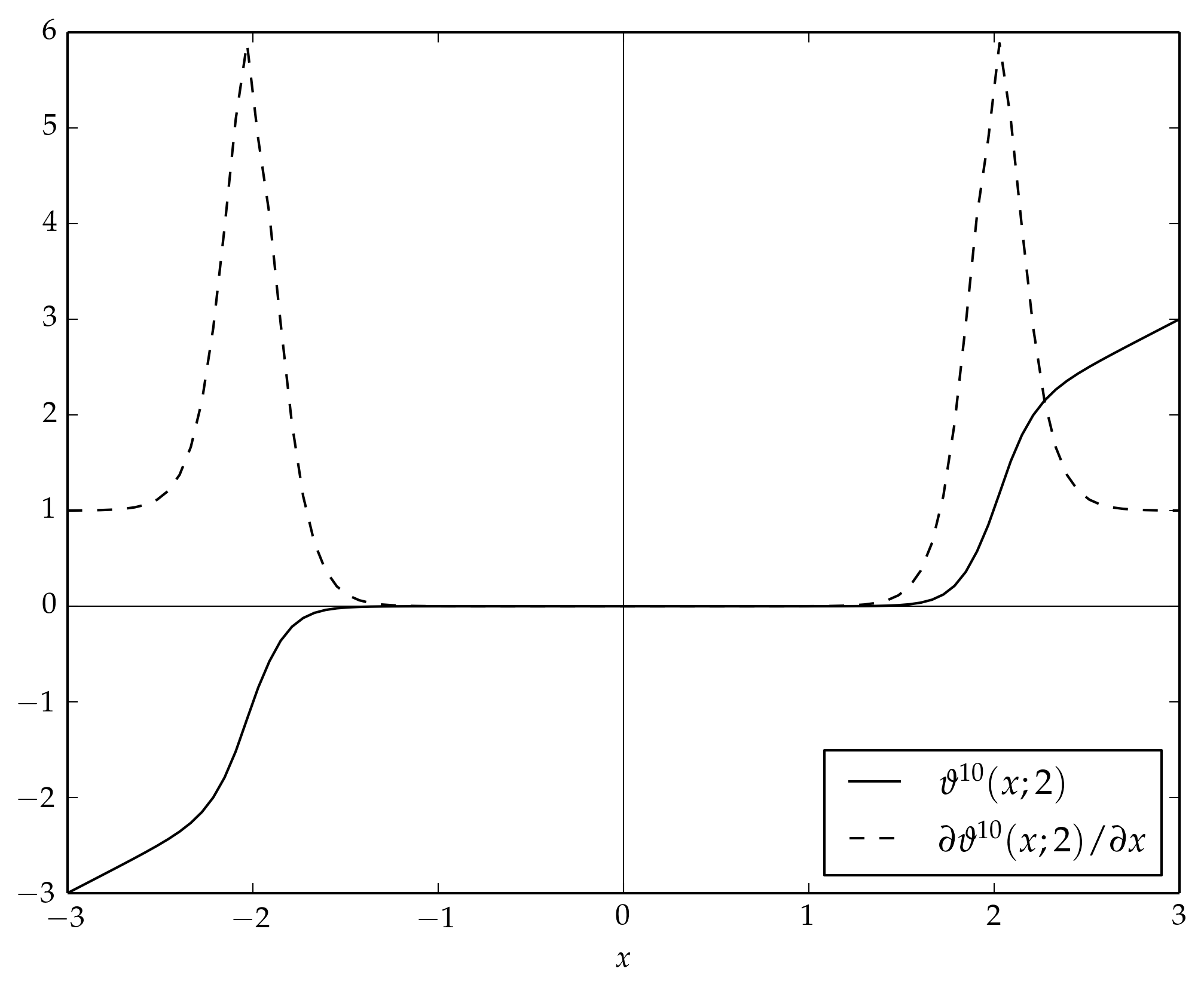
(a) The solid line represents the function $\vartheta^{10}(x;2)$. The dashed line represents its derivative with respect to $x$.

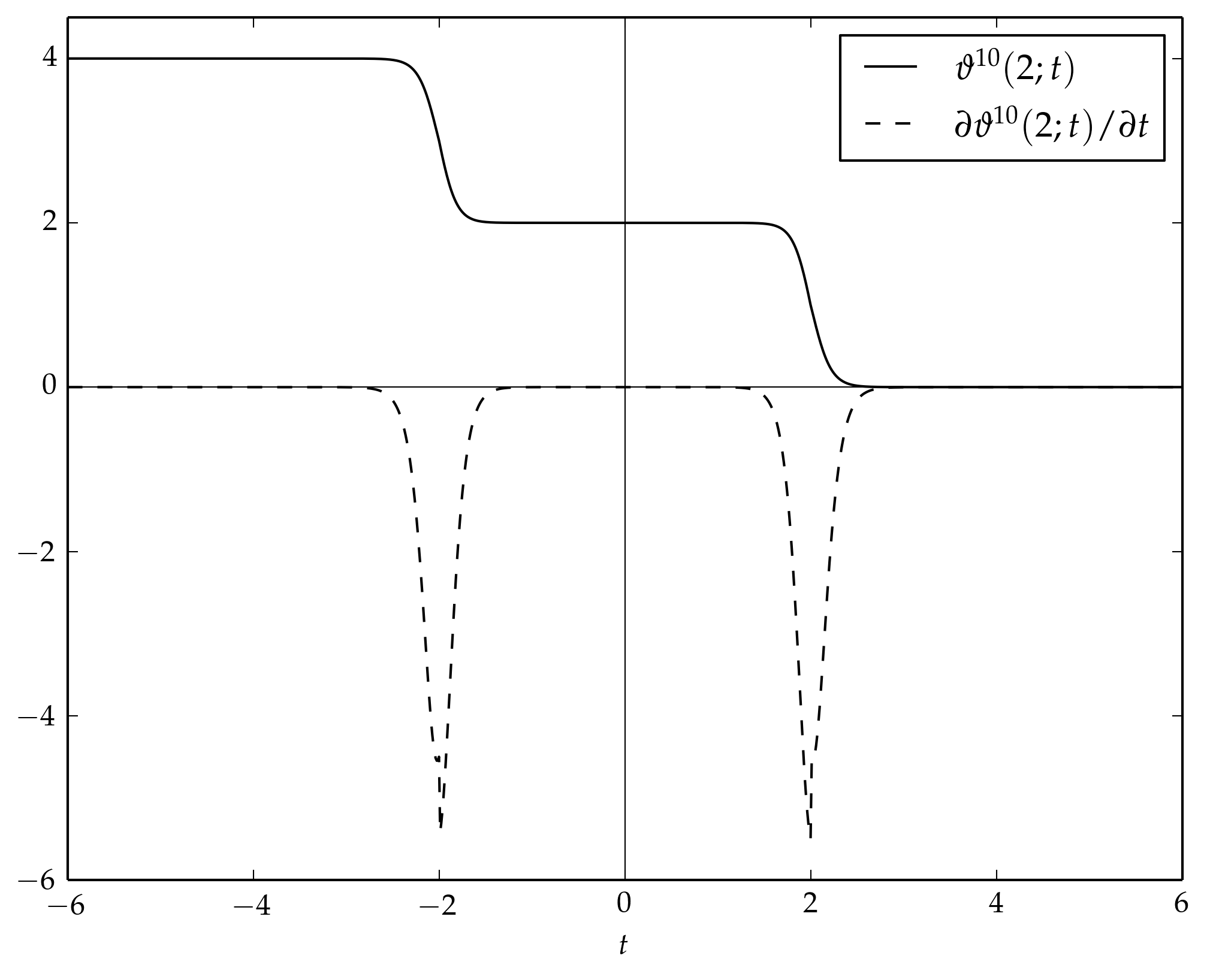
(b) The solid line represents the function $\vartheta^{10}(2;t)$. The dashed line represents its derivative with respect to $t$.

Figure 1: Representation of the function $\vartheta^{\alpha}$ of Equation (1).

Definition 1 (Pruning function)

The pruning function $\vartheta^{\alpha}(\cdot;t)$, needed for the compression procedure, is defined as follows:

$$\vartheta^{\alpha}(x;t)\coloneqq \hphantom{-.}\operatorname{ReLU}(x-t)+t\cdot\sigma(\alpha(x-t))+$$ (1)

$$-\operatorname{ReLU}(-x-t)-t\cdot\sigma(\alpha(-x-t)),$$

where $\alpha$ and $t$ are positive real numbers, $\sigma$ is the sigmoidal function $\sigma(x)\coloneqq{(1+\mathrm{e}^{\textrm{-}x})}^{\textrm{-}1}$, and $\operatorname{ReLU}(x)\coloneqq\max(0,x)$ is the Rectified Linear Unit function (see Figure 1).

Note that, the purpose of the pruning function is to force toward zero all the elements of the domain within $(-t-\Delta,+t+\Delta)$ (for a suitable $\mathbb{R}\ni\Delta\geq 0$); the variable $t$ acts then as a threshold variable. On the other hand, the parameter $\alpha$ determines the speed how quickly the pruning takes place within such interval.

We are now showing that $\vartheta^{\alpha}$ is learnable with respect to the variables $x$ and $t$. The (weak) partial derivatives of $\vartheta^{\alpha}$ with respect of $x$ and $t$ are given by:

$$\frac{\partial\vartheta^{\alpha}}{\partial x}= H(x-t)+H(-x-t)+$$

$$+\alpha t\cdot\sigma(\alpha(x-t))[1-\sigma(\alpha(x-t))]+$$

$$+\alpha t\cdot\sigma(\alpha(-x-t))[1-\sigma(\alpha(-x-t))],$$ (2)

$$\frac{\partial\vartheta^{\alpha}}{\partial t}= -H(x-t)+H(-x-t)+$$

$$+\sigma(\alpha(x-t))-\sigma(\alpha(-x-t))+$$

$$-\alpha t\cdot\sigma(\alpha(x-t))[1-\sigma(\alpha(x-t))]+$$

$$+\alpha t\cdot\sigma(\alpha(-x-t))[1-\sigma(\alpha(-x-t))],$$ (3)

where $H(x)$ is the Heaviside step function: $H(x)=1$ if $x\geq 0$, $H(x)=0$ otherwise. Equations (2) and (3) show that the (weak) partial derivatives of $\vartheta^{\alpha}(x;t)$ are different than zero almost everywhere, thus allowing the parameter $t$ to be learnable by means of gradient descent (see also Figure 1).

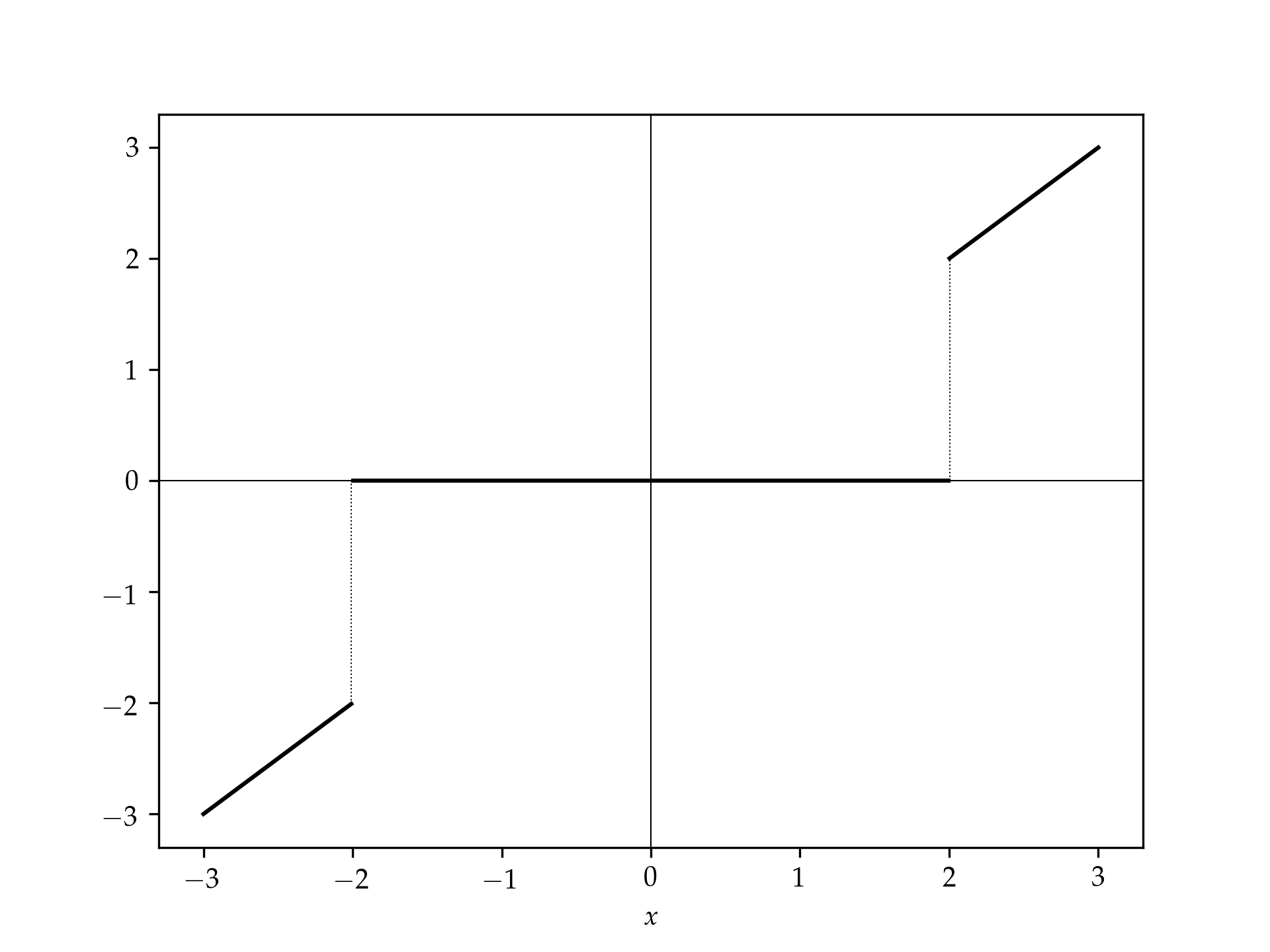
(a) The function $\bar{\vartheta}(x;2)$.

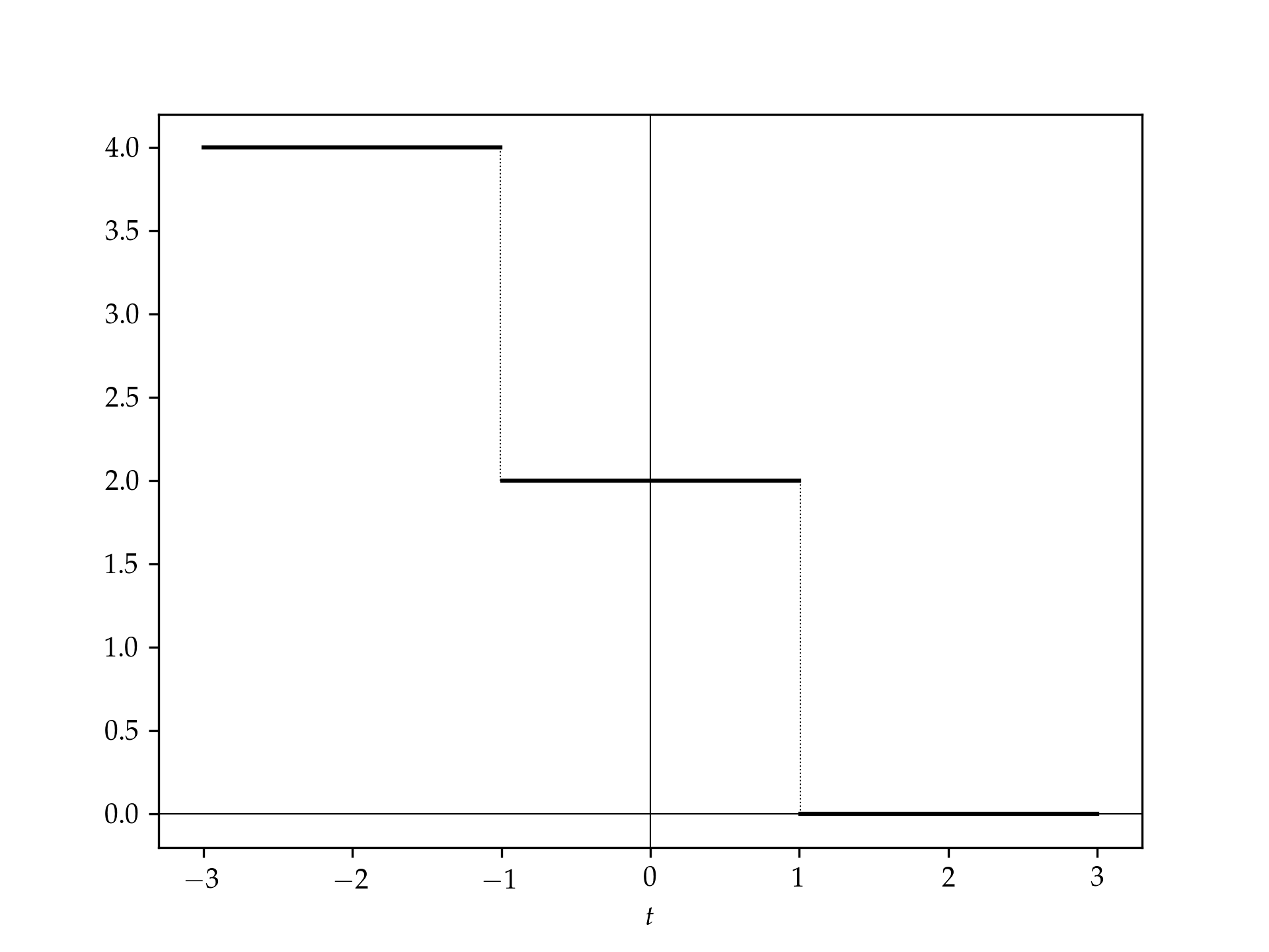
(b) The function $\bar{\vartheta}(2;t)$.

Figure 2: The graph of the function $\bar{\vartheta}(x;t)$ of Equation (2). Note how the derivative with respect of $t$ is zero almost everywhere.

It is interesting to notice that, $\vartheta^{\alpha}(\,\cdot\,;t)$ is a smoothed version of the thresholded linear function $\bar{\vartheta}(\cdot;t)$.

Definition 2 (Thresholded linear function)

The thresholded linear function $\bar{\vartheta}(\cdot;t)$ is defined as follow [23, 24]:

$$\bar{\vartheta}(x;t)\coloneqq \hphantom{-.}\operatorname{ReLU}(x-t)+t\cdot H(x-t)+\phantom{.}$$

$$-\operatorname{ReLU}(-x-t)-t\cdot H(-x-t).$$ (4)

Note that, $\vartheta^{\alpha}(x;t)$ converges weakly to $\bar{\vartheta}(x;t)$ when $\alpha\to\infty$. Moreover, the weak partial derivatives of $\bar{\vartheta}(x;t)$ with respect to $x$ and $t$ are:

$$\frac{\partial\bar{\vartheta}}{\partial x}=H(x-t)+t\cdot\delta(x-t)+H(-x-t)+t\cdot\delta(x+t),$$

$$\frac{\partial\bar{\vartheta}}{\partial t}=-t\cdot\delta(x-t)+t\cdot\delta(x+t),$$

where $\delta$ is the Dirac’s delta, thus forbidding any sort of learning procedure on the variable $t$ (see Figure 2).

III-B Sibling networks

III-B1 Building

Given a network $N=L[{\bm{\mathcal{W}}}_{d}]\circ\ldots\circ L[{\bm{\mathcal{W}}}_{1}]$, the sibling network $N_{\text{s}}$ is defined as follows:

$$N_{\text{s}}\coloneqq L[\vartheta^{\alpha}({\bm{\mathcal{W}}}_{d};t_{d})]\circ\ldots\circ L[\vartheta^{\alpha}({\bm{\mathcal{W}}}_{1};t_{1})].$$ (5)

Note that, in the equations for the networks $N$ and $N_{\text{s}}$ we did not specify the type of each layer so to reduce the clutter in the notation. Moreover, in the previous equation $\alpha$ is an hyper-parameter, while all the $t_{i}$ are learnable weights. For the sake of the clarity, we are assuming one threshold variable per layer, as well as that there is one $\alpha$ hyper-parameter shared by all the layers. These simplifying assumptions can be easily relaxed.

III-B2 Training

The learning of all the $\bm{W}_{j}$ and $t_{j}$ of the sibling network $N_{\text{s}}$ is performed by means of gradient descent. The loss function to be minimized is given by $\mathcal{L}\coloneqq\mathcal{L}_{0}+\mathcal{L}_{\text{wd}}+\mathcal{L}_{t}$, with $\mathcal{L}_{0}$ the basic loss function for the problem under analysis (e.g. cross-entropy), where:

$$\mathcal{L}_{\text{wd}}\coloneqq\lambda_{\text{wd}}\sum_{i}\sum_{\bm{W}_{j}\in{\bm{\mathcal{W}}}_{i}}\left\lVert\bm{W}_{j}\right\rVert_{2}^{2},$$

$$\mathcal{L}_{t}\coloneqq\lambda_{t}\sum_{i}\sum_{j\mid\bm{W}_{j}\in{\bm{\mathcal{W}}}_{i}}\left\lVert\vartheta^{\alpha}(\bm{W}_{j};t_{j})\right\rVert_{1},$$ (6)

with $\left\lVert\bm{X}\right\rVert_{p}$ the entry-wise $p$-norm of the matrix $\bm{X}$. Namely,

1. $\mathcal{L}_{\text{wd}}$ is the usual weight decay regularizer on all the $\bm{W}_{j}$ variables, with $\lambda_{\text{wd}}$ the corresponding hyper-parameter;

2. $\mathcal{L}_{t}$ is a regularizer used to speed-up pruning, where $\lambda_{t}$ is its hyper-parameter.

The optimization of the training function is performed using one variant of stochastic gradient descent, with the following caveats:

1. the regularizer $\mathcal{L}_{t}$ is optimized only with respect to all the variables $t_{j}$, i.e. the contribution to the gradient given by $\mathcal{L}_{t}$ with respect to all the $\bm{W}_{j}$ is zero;

2. the learning rate of all the variables $t_{j}$ is slowed by a factor $\rho$ so to reduce the effective learning rate of the thresholds with respect to the other parameters;

3. the learning of all $t_{j}$ is performed by enforcing non-negativity;

4. weights are initialized randomly as in a customary neural network (e.g. Glorot initialization [25]), while initial values of the thresholds are set such that a small amount $p$ (e.g. $0\%\div 10\%$) of weights are effectively below the threshold at the beginning of the training.

The purpose of the regularizer $\mathcal{L}_{t}$ is to enforce sparsity of the weights under the mapping of the pruning function $\vartheta^{\alpha}$. Since it affects only the learning of all the thresholds $t_{j}$ (i.e. it is not involved in the partial derivative of the loss with respect to any ${\boldsymbol{W}}_{j}$), it effectively moves the pruning thresholds so to increase the after-mapping sparsity. Instead, the weight decay regularizer $\mathcal{L}_{\text{wd}}$ is used to enforce the weights to gather around all the threshold values $t_{j}$ (see Figure 3 in Section IV-A1 for a comparison between the distribution of the learned weights of the first layer of a LeNet-300-100 on MNIST with and without the $\mathcal{L}_{\text{wd}}$ regularizer).

III-B3 Pruning

The sibling networks $N_{\text{s}}$ learned accordingly to Section III-B2 has few zero weights, due to the smooth behavior of the function $\vartheta^{\alpha}$ that we used to enforce weights shrinking. However, thanks to the $\vartheta^{\alpha}$ itself, many of the weights of the network $N_{\text{s}}$ are near zero. For this reason, we get an actual pruned network $N_{\text{p}}$ from $N_{\text{s}}$ by setting to zero all the learned weights of $N_{\text{s}}$ that under the mapping of $\theta^{\alpha}$ are below a certain (small) cutoff value $\gamma$, which has to be considered as a hyper-parameter. We found out empirically that $\gamma\sim 10^{\textrm{-}3}$ is a good starting choice in almost all the cases.

Precisely, denoting with $\widetilde{{\bm{\mathcal{W}}}}_{j}$ the weights learned during the training phase of the sibling network and with $\tilde{t}_{j}$ the learned threshold parameters, the pruned network $N_{\text{p}}$ is given by:

$$N_{\text{p}}\coloneqq L[\vartheta^{\alpha}_{\text{inv}}(\bar{\vartheta}(\vartheta^{\alpha}(\widetilde{{\bm{\mathcal{W}}}}_{d};\tilde{t}_{d});\gamma);\tilde{t}_{d})]\circ$$ (7)

$$\ldots\circ L[\vartheta^{\alpha}_{\text{inv}}(\bar{\vartheta}(\vartheta^{\alpha}(\widetilde{{\bm{\mathcal{W}}}}_{1};\tilde{t}_{1});\gamma);\tilde{t}_{1})],$$

where $\vartheta^{\alpha}_{\text{inv}}(x;t)$ is the inverse function of $\vartheta^{\alpha}(x;t)$ with respect to $x$ when $t$ is given. Note that $\vartheta^{\alpha}_{\text{inv}}$ exists, since $\vartheta^{\alpha}$ is bijective. Moreover, since $\vartheta^{\alpha}(0;t)=0$ we have that $\vartheta^{\alpha}_{\text{inv}}(0;t)=0$.

IV Results

The experiments we performed can be split in two groups:

1. we pruned LeNet-300-100 and LeNet-5 on MNIST dataset, as well as AlexNet on ILSVRC-2012 dataset; for these networks we assessed the compression ratio due to pruning as well as the drop in accuracy against their non-pruned counterparts (see Section IV-A);

2. for the pruned AlexNet on ILSVRC-2012 we studied the generalization performance in the transfer learning scenario considering different recognition tasks, such as object image classification, scene recognition, fine grained recognition, attribute detection, and image retrieval (see Section IV-B).

IV-A Pruning

We pruned LeNet-300-100 and LeNet-5 on MNIST dataset, and AlexNet on ILSVRC-2012 dataset.

MNIST is a large database of gray-scale handwritten digits, made of 60K training images and 10K testing images [26]. On the other hand, the ILSVRC-2012 dataset is a 1000 classes classification task with 1.2M training examples and 50k validation examples.

All our networks were built and trained using the Keras framework [27] on top of TensorFlow [28]. The size of the networks and their accuracy before and after pruning are shown in Table I, together with the performance achieved by Han et al. in [2], the paper of Deep Compression focusing on the pruning stage of the compression pipeline. The technique presented in this paper keeps the error rate of the pruned networks comparable to the non-pruned counterparts as in the current state-of-the-art, while achieving better pruning rate. In the experiments we performed, our pruning technique saved network storage by $12\times$ to $19\times$ across different networks, thus increasing Han et al. compression rate by a factor $\approx\!1.3\times$ to $\approx\!1.6\times$ and reducing by $14\%$ to $33\%$ the number of weights retained by Deep Compression.

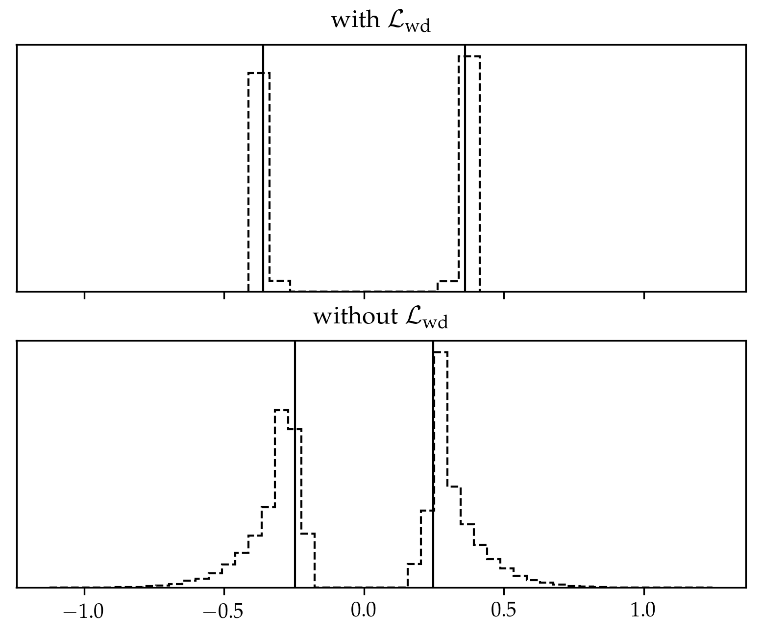
Figure 3: The figure shows the distribution of the trained weights of the first layer of two pruned LeNet-300-100 on MNIST, with $\alpha=100$ and a cutoff $\gamma=10^{\textrm{-}3}$. The vertical solid lines represent the learned thresholds. The top plot was trained with weight decay regularizer, while the bottom one without it. Note how in the first case the weights group around the threshold values.

IV-A1 LeNet-300-100 and LeNet-5 on MNIST

We first experimented on MNIST dataset with LeNet-300-100 and LeNet-5 networks [7]. LeNet-300-100 is a fully connected network made of two hidden layers, with 300 and 100 neurons respectively, achieving $1\%\!\div\!2\%$ error rate on MNIST.

LeNet-5 is a convolutional network that has two convolutional layers and two fully connected layers, achieving $<1\%$ error rate on MNIST. All the convolutional layers of LeNet-5 have been pruned by learning a different threshold weight per filter, thus partially relaxing the simplifying assumption we used to write Equation (5).

All the networks were trained using Adam optimizer [29] with learning rate $10^{\textrm{-}3}$. In addition, pruned networks were learned with the following configuration of the hyper-parameters: $\alpha=10^{2}$, $p=10^{\textrm{-}1}$, $\rho=\lambda_{t}=10^{\textrm{-}2}$, $\gamma=10^{\textrm{-}3}$, $\lambda_{\text{wd}}=10^{\textrm{-}4}$.

Table I shows that these networks on MNIST can be pruned with basically no drop in accuracy with the respect of their non-compressed counterparts. The pruning procedure achieves a storage saving of $15\!\times$ and $19\!\times$, reducing by 33% (7K) and 14% (14K) the number of weights retained by Deep Compression, for LeNet-300-100 and LeNet-5 respectively.

Table II shows the per-layer statistics of the pruning procedure. It is interesting to notice that, our approach converged to a network configuration where the pruning ratio is significantly higher for the biggest layers.

Figure 3 shows the comparison between the distribution of the first layer weights of a LeNet-300-100 with and without weight-decay. It is possible to notice that, the weights are much more gathered around the learned threshold when the weight-decay parameter is used during the learning process. We speculate such a grouping might make weights quantization in Deep Compression [1] more efficient.

IV-A2 AlexNet on ILSVRC-2012

We implemented the original AlexNet model [30] from scratch using the Keras framework. The training of the non-pruned and pruned AlexNet were performed using stochastic gradient descent with starting learning rate $10^{\textrm{-}2}$, step-wise learning rate decay, learning rate multiplier equal to $2$ for all the bias weights, weight-decay hyper-parameter $\lambda_{\text{wd}}=5\cdot 10^{\textrm{-}4}$, and momentum $0.9$, exactly as in the original paper [30]. On the other hand, the compression procedure was carried out with the hyper-parameters $\alpha=10^{2}$, $p=0$, $\rho=10^{\textrm{-}11}$, $\lambda_{t}=10^{\textrm{-}2}$, $\gamma=10^{\textrm{-}3}$.

Network	$\Delta_{1}$ Err.	$\Delta_{5}$ Err.	Weights	Pruning
LeNet-300-100 reference	—	—	266K	—
LeNet-300-100 pruned (Han et al.)	$\approx\!-0.1\%$	—	21K	$12\times$
LeNet-300-100 pruned (this paper)	$\approx\!+0.1\%$	—	$\bm{14\text{K}}$	$\bm{19\times}$
LeNet-5 reference	—	—	431K	—
LeNet-5 pruned (Han et al.)	$\approx\!-0.1\%$	—	34K	$12\times$
LeNet-5 pruned (this paper)	$\approx\!-0.0\%$	—	$\bm{29\text{K}}$	$\bm{15\times}$
AlexNet reference	—	—	61M	—
AlexNet pruned (Han et al.)	$\approx\!-0.0\%$	$\approx\!-0.0\%$	7M	$9\times$
AlexNet pruned (this paper)	$\approx\!+1.1\%$	$\approx\!+1.0\%$	$\bm{5\text{M}}$	$\bm{12\times}$

TABLE I: The table shows the difference in Top-1 ($\Delta_{1}$) and Top-5 ($\Delta_{5}$) errors between the networks pruned in this paper and their reference non-pruned implementation. It also shows the pruning performance. Similarly, it is also shown $\Delta_{1}$/$\Delta_{5}$ and pruning rate achieved by Han et al. in [2].

	LeNet-300-100
	fc1			fc2			fc3		total
Weights	235K			30K			1K		431K
Pruning	94.7%			83.8%			11.9%		94.7%
	19$\times$			6$\times$			1$\times$		19$\times$
	LeNet-5
	conv1		conv2		fc3		fc4		total
Weights	0.5K		25K		400K		1K		431K
Pruning	31.1%		82.2%		96.6%		41.7%		93.3%
	1$\times$		6$\times$		29$\times$		2$\times$		15$\times$
	AlexNet
	conv1	conv2	conv3	conv4	conv5	fc6	fc7	fc8	tot
Weights	35K	307K	885K	663K	442K	38M	17M	4M	61M
Pruning	3.8%	34.9%	24.3%	36.7%	33.5%	96.8%	91.5%	78.5%	91.5%
	$1\times$	$2\times$	$1\times$	$2\times$	$2\times$	$31\times$	$12\times$	$5\times$	$12\times$

TABLE II: The table shows how the pruning rate behaves for each layer of LeNet-300-100 and LeNet-5 trained on MNIST, and AlexNet trained on ILSVRC-2012.

Table I shows that our procedure can achieve a memory saving of about $12\!\times$, with a small drop in the accuracy compared to the non-compressed counterpart (i.e. $\approx\!1.1\%$ top-1 and $\approx\!1.0\%$ top-5). Such a pruning performance translates into a reduction of 2M (29%) weights compared to the number of weights retained by Deep Compression.

Table II shows the per-layer statistics of the pruning procedure. Again, our approach converged to a network compression where the pruning ratio is significantly higher for the biggest layers of the networks, with a staggering $31\!\times$ for the biggest layer of the network, i.e. fc6.

Task	Dataset	Performance Measure	Uncompressed	Compressed	Difference
Image classification	Pascal VOC 2007 [31]	mean Average Precision (mAP)	0.6235	0.6132	-0.0103
	MIT-67 indoor scenes [32]	Accuracy	0.5440	0.5425	-0.0015
Fine grained recognition	Birds (CUB) 200-2011 [33]	Accuracy	0.5043	0.5173	0.0130
	Oxford 102 flowers [34]	Accuracy	0.8477	0.8542	0.0065
Attribute detection	UIUC 64 objects attributes [35]	mean Area Under Curve (mAUC)	0.7999	0.7953	-0.0046
	H3D person attributes [36]	mean Average Precision (mAP)	0.5664	0.5646	-0.0018
Visual instance retrieval	Oxford5k buildings [37]	mean Average Precision (mAP)	0.3471	0.3901	0.0430
	Paris6k buildings [38]	mean Average Precision (mAP)	0.5958	0.6007	0.0049
	Sculptures6k [39]	mean Average Precision (mAP)	0.3093	0.2982	-0.0111
	Holidays dataset [40]	mean Average Precision (mAP)	0.7302	0.7187	-0.0115
	UKbench [41]	Recall@4	0.8770	0.8904	0.0134

TABLE III: Transfer learning performance of the features extracted from the AlexNet network trained and compressed on ImageNet ILSVRC-2012 compared to those extracted from the same uncompressed network. The comparison is performed on different recognition tasks: object image classification, scene recognition, fine grained recognition, attribute detection and image retrieval applied to a diverse set of datasets.

IV-B Transfer Learning

In the previous section we showed that we are able to heavily compress a deep neural network keeping the same recognition performance on the training dataset. Since CNN are very often used for transfer learning as feature extractors due to the the effectiveness and generality of the learned representations [3], in this section we investigate how the compressed features perform on various recognition tasks and different datasets. We used features extracted from the AlexNet network trained and compressed on ILSVRC-2012 dataset as a generic image representation to tackle the diverse range of recognition tasks tested in [3], i.e.: object image classification, scene recognition, fine grained recognition, attribute detection and image retrieval applied to many datasets.

For all the experiments we resized the input image to $227\times 227$ and we used the last fully connected layer (i.e. layer fc7) of the network as our feature vector. This gives a vector of 4096 dimension that is further $L2$ normalized to unit length for all the experiments. For all the different classification and recognition tasks considered we used the 4096 dimensional feature vector in combination with a linear Support Vector Machine [42, 43]. For visual instance retrieval task we adopted the Euclidean distance to compute the visual similarity between a query and the images from target dataset.

IV-B1 Image Classification

The first problem faced was image classification of objects and scenes. The task is to assign (potentially multiple) semantic labels to an image. Two datasets were considered for two different recognition tasks: the Pascal VOC 2007 for object image classification [31] and the MIT-67 indoor scenes [32] for scene recognition. The results are reported in Table III, where it can be seen that the compressed features have almost the same transfer learning performance of the non-compressed ones, with a drop in mean Average Precision (mAP) on Pascal VOC 2007 of $\approx\!1.0\%$ and a drop in accuracy on MIT-67 of $\approx\!0.2\%$.

IV-B2 Fine Grained Recognition

The second problem faced was fine grained recognition that involves recognizing sub-classes of the same object class such as different bird species, dog breeds, flower types, etc. The task is different from the one faced in Sec. IV-B1 since the differences across different subordinate classes are very subtle and they require a fine-detailed representation. We evaluated the compressed CNN features on two fine-grained recognition datasets: Caltech-UCSD Birds (CUB) 200-2011 [33] and Oxford 102 flowers [34]. The results are reported in Table III, where it can be seen that the compressed features have slightly better transfer learning performance of the non-compressed ones, with an increase in accuracy of $\approx\!1.3\%$ and $\approx\!0.7\%$ on Caltech-UCSD Birds and Oxford 102 flowers respectively.

IV-B3 Attribute Detection

The third problem faced was attribute detection, which in the context of computer vision is defined as the detection of some semantic or abstract quality shared by different instances/categories. We used two datasets for attribute detection: the UIUC 64 object attributes dataset [35] and the H3D dataset [36] which defines 9 attributes for a subset of the person images from Pascal VOC 2007. The results are reported in Table III, where it can be seen that the compressed features have almost the same transfer learning performance of the non-compressed ones, with a drop in mean Area Under Curve (mAUC) on UIUC 64 of $\approx\!0.5\%$ and a drop in mAP on H3D of $\approx\!0.2\%$.

IV-B4 Visual Instance Retrieval

The fourth problem faced was visual instance retrieval, which consists in retrieving from a given target dataset the most similar images to a given query image. The similarity between images was obtained as the Euclidean distance between the corresponding feature vectors. The ground truth was defined as the set of the target database images that were relevant or not relevant to a given query.

We considered five datasets from the state-of-the-art:

1. Oxford5k buildings [37]: this is a collection of images depicting buildings from the city of Oxford with 55 query and 5063 target images. This retrieval task is quite challenging because the visual appearance of Oxford buildings is very similar;

2. Paris6k buildings [38]: this is a collection of images depicting buildings and monuments from the city of Paris with 55 query and 6412 target images. This task is less challenging then the previous one because the images of the dataset are more diverse than those in Oxford5k;

3. Sculptures6k [39]: This collection contains 6340 images of sculptures by Moore and Rodin, divided in train and test (with 70 query images);

4. Holidays dataset [40]: this collection contains 1491 images (with 500 query images) of different scenes, items and monuments. The images are quite diverse, so this dataset is less challenging than the previous ones. The performance for all the above datasets was assessed by calculating the mAP;

5. UKbench [41] this collection contains 2250 items, each from four different viewpoints with a total of 10200 images. Each image of the collection is used as a query and we assessed the performance using the Recall at top four (Recall@4).

The results for the visual instance retrieval problem are reported in Table III. It can be seen that, also in this case, the compressed features have almost the same transfer learning performance of the non-compressed ones, with a drop in mAP on Sculptures6k and Holidays of $\approx\!0.1\%$. On the other three datasets instead we can observe a slight improvement in performance with an increase of $\approx\!4.3\%$ and $\approx\!0.5\%$ in mAP on Oxford5k buildings and Paris6k buildings respectively, and of $\approx\!1.3\%$ in Recall@4 on UKbench.

From all the recognition experiments considered, we note that, on average, there is no loss in transfer learning performance of the compressed features compared to the non-compressed ones. This phenomenon might be explained by [44]. In their work, the authors Shwartz-Ziv and Tishby showed that the training process of deep neural networks is characterized by two distinct phases: the first one consists into fast drift, in which the training error is reduced; the second one involves stochastic relaxation (i.e. random diffusion) constrained by the training error value. This second phase leads to a decrease of the mutual information between the probability distributions of each layer weights and inputs, i.e. an implicit compression of the representations.

V Conclusion

We presented a method to improve the pruning step of the current state-of-the-art methodology to compress neural networks: Deep Compression [1]. The proposed approach is general purpose, and it can be easily applied to all network architectures.

The novelty of our technique lies in differentiability of the pruning phase with respect to the thresholds, thus allowing pruning during the backward phase of the learning procedure and exploiting regular gradient descent techniques for the whole pruning phase. Moreover, since the thresholds are learnable, the backpropagation can jointly optimize on both the network weights and the pruning thresholds. Furthermore, since there is a threshold per layer (or per filter), every layer (filter) can be optimized independently of all the other ones. As far as we know, this is the first approach able to jointly prune and learn network weights.

We showed that the proposed compression pipeline improves the current state-of-the-art regarding pruning rate (up to $19\!\times$ compression due to pruning for small networks on MNIST, and $12\!\times$ compression for a big network on ILSVRC-2012), with no or negligible drop in network accuracy and strongly reducing the training time. This leads to smaller memory capacity and bandwidth requirements for real-time image processing, making it easier to be deployed on mobile systems.

Moreover, we showed in a transfer learning scenario that the compression phase does not alter the effectiveness and generality of the learned representations, obtaining in the worst case a negligible drop in performance of $\approx\!1.2\%$ and in the best case an improvement of $\approx\!4.3\%$. This was verified on the wide range of recognition tasks identified in [3] on a diverse set of datasets: object image classification (Pascal VOC 2007), scene recognition (MIT-67 indoor scenes), fine grained recognition (Birds CUB 200-2011 and Oxford 102 flowers), attribute detection (UIUC 64 objects attributes and H3D person attributes) and image retrieval (Oxford5k buildings, Paris6k buildings, Sculptures6k, Holidays dataset and UKbench). We believe that, this is the first work where the generalization properties of compressed networks have been analyzed.

In our opinion, interesting extensions of this work are: (i) further testing the pruning technique proposed in this paper by considering e.g. other big networks (VGG) or small more recent networks (ResNet); (ii) quantizing and Huffman coding the pruned network, so to mimic the full compression pipeline proposed by Deep Compression; (iii) comparing the generalization capabilities of the networks pruned with our technique with ones compressed by Deep Compression; (iv) devising a differentiable quantization technique, so to achieve a pruning+quantization step learnable by stochastic gradient descent methods.

References

- [1] S. Han, H. Mao, and W. J. Dally, “Deep Compression: Compressing Deep Neural Networks with Pruning, Trained Quantization and Huffman Coding,” in ICLR, 2016.
- [2] S. Han, J. Pool, J. Tran, and W. Dally, “Learning both weights and connections for efficient neural network,” in Advances in Neural Information Processing Systems, 2015, pp. 1135–1143.
- [3] A. Sharif Razavian, H. Azizpour, J. Sullivan, and S. Carlsson, “Cnn features off-the-shelf: an astounding baseline for recognition,” in Proceedings of the IEEE conference on computer vision and pattern recognition workshops, 2014, pp. 806–813.
- [4] M. Denil, B. Shakibi, L. Dinh, N. de Freitas et al., “Predicting parameters in deep learning,” in Advances in Neural Information Processing Systems, 2013, pp. 2148–2156.
- [5] A. Coates, A. Ng, and H. Lee, “An analysis of single-layer networks in unsupervised feature learning,” in Proceedings of the fourteenth international conference on artificial intelligence and statistics, 2011, pp. 215–223.
- [6] K. Gregor and Y. LeCun, “Emergence of complex-like cells in a temporal product network with local receptive fields,” arXiv preprint arXiv:1006.0448, 2010.
- [7] Y. LeCun, L. Bottou, Y. Bengio, and P. Haffner, “Gradient-based learning applied to document recognition,” Proceedings of the IEEE, vol. 86, no. 11, pp. 2278–2324, 1998.
- [8] W. Chen, J. Wilson, S. Tyree, K. Weinberger, and Y. Chen, “Compressing neural networks with the hashing trick,” in International Conference on Machine Learning, 2015, pp. 2285–2294.
- [9] E. L. Denton, W. Zaremba, J. Bruna, Y. LeCun, and R. Fergus, “Exploiting linear structure within convolutional networks for efficient evaluation,” in Advances in Neural Information Processing Systems, 2014, pp. 1269–1277.
- [10] S. J. Hanson and L. Y. Pratt, “Comparing biases for minimal network construction with back-propagation,” in Advances in neural information processing systems, 1989, pp. 177–185.
- [11] Y. L. Cun, J. S. Denker, and S. A. Solla, “Optimal brain damage,” in Advances in Neural Information Processing Systems, D. S. Touretzky, Ed. San Francisco, CA, USA: Morgan Kaufmann Publishers Inc., 1990, pp. 598–605. [Online]. Available: http://dl.acm.org/citation.cfm?id=109230.109298
- [12] B. Hassibi, D. G. Stork, and G. J. Wolff, “Optimal brain surgeon and general network pruning,” in Neural Networks, 1993., IEEE International Conference on. IEEE, 1993, pp. 293–299.
- [13] S. Han, X. Liu, H. Mao, J. Pu, A. Pedram, M. A. Horowitz, and W. J. Dally, “Eie: Efficient inference engine on compressed deep neural network,” in Proceedings of the 43rd International Symposium on Computer Architecture, ser. ISCA ’16. Piscataway, NJ, USA: IEEE Press, 2016, pp. 243–254. [Online]. Available: https://doi.org/10.1109/ISCA.2016.30
- [14] Y. Gong, L. Liu, M. Yang, and L. Bourdev, “Compressing deep convolutional networks using vector quantization,” arXiv preprint arXiv:1412.6115, 2014.
- [15] K. Hwang and W. Sung, “Fixed-point feedforward deep neural network design using weights+ 1, 0, and- 1,” in Signal Processing Systems (SiPS), 2014 IEEE Workshop on. IEEE, 2014, pp. 1–6.
- [16] V. Vanhoucke, A. Senior, and M. Z. Mao, “Improving the speed of neural networks on CPUs,” in Proc. Deep Learning and Unsupervised Feature Learning NIPS Workshop, vol. 1, 2011, p. 4.
- [17] M. Courbariaux, Y. Bengio, and J.-P. David, “Binaryconnect: Training deep neural networks with binary weights during propagations,” in Advances in Neural Information Processing Systems, 2015, pp. 3123–3131.
- [18] I. Hubara, M. Courbariaux, D. Soudry, R. El-Yaniv, and Y. Bengio, “Binarized neural networks,” in Advances in Neural Information Processing Systems 29, 2016, pp. 4107–4115.
- [19] M. Rastegari, V. Ordonez, J. Redmon, and A. Farhadi, “Xnor-net: Imagenet classification using binary convolutional neural networks,” in European Conference on Computer Vision. Springer, 2016, pp. 525–542.
- [20] R. S. Michalski, “A theory and methodology of inductive learning,” Artificial intelligence, vol. 20, no. 2, pp. 111–161, 1983.
- [21] S. Thrun and L. Pratt, Learning to learn. Springer Science & Business Media, 2012.
- [22] J. Yosinski, J. Clune, Y. Bengio, and H. Lipson, “How transferable are features in deep neural networks?” in Advances in neural information processing systems, 2014, pp. 3320–3328.
- [23] C. J. Rozell, D. H. Johnson, R. G. Baraniuk, and B. A. Olshausen, “Sparse coding via thresholding and local competition in neural circuits,” Neural computation, vol. 20, no. 10, pp. 2526–2563, 2008.
- [24] K. Konda, R. Memisevic, and D. Krueger, “Zero-bias autoencoders and the benefits of co-adapting features,” arXiv preprint arXiv:1402.3337, 2014.
- [25] X. Glorot and Y. Bengio, “Understanding the difficulty of training deep feedforward neural networks,” in Proceedings of the Thirteenth International Conference on Artificial Intelligence and Statistics, 2010, pp. 249–256.
- [26] Y. LeCun, “The MNIST database of handwritten digits,” 1998.
- [27] F. Chollet et al., “Keras,” https://github.com/fchollet/keras, 2015.
- [28] M. Abadi, P. Barham, J. Chen, Z. Chen, A. Davis, J. Dean, M. Devin, S. Ghemawat, G. Irving, M. Isard et al., “Tensorflow: A system for large-scale machine learning.” in OSDI, vol. 16, 2016, pp. 265–283.
- [29] D. P. Kingma and J. Ba, “Adam: A Method for Stochastic Optimization,” in ICLR, dec 2015. [Online]. Available: http://arxiv.org/abs/1412.6980
- [30] A. Krizhevsky, I. Sutskever, and G. E. Hinton, “Imagenet classification with deep convolutional neural networks,” in Advances in neural information processing systems, 2012, pp. 1097–1105.
- [31] M. Everingham, L. Van Gool, C. Williams, J. Winn, and A. Zisserman, “The pascal visual object classes challenge 2012 (voc2012) results (2012),” in URL http://www. pascal-network. org/challenges/VOC/voc2011/workshop/index. html, 2011.
- [32] A. Quattoni and A. Torralba, “Recognizing indoor scenes,” in Computer Vision and Pattern Recognition, 2009. CVPR 2009. IEEE Conference on. IEEE, 2009, pp. 413–420.
- [33] C. Wah, S. Branson, P. Welinder, P. Perona, and S. Belongie, “The caltech-ucsd birds-200-2011 dataset,” 2011.
- [34] M.-E. Nilsback and A. Zisserman, “Automated flower classification over a large number of classes,” in Computer Vision, Graphics & Image Processing, 2008. ICVGIP’08. Sixth Indian Conference on. IEEE, 2008, pp. 722–729.
- [35] A. Farhadi, I. Endres, D. Hoiem, and D. Forsyth, “Describing objects by their attributes,” in Computer Vision and Pattern Recognition, 2009. CVPR 2009. IEEE Conference on. IEEE, 2009, pp. 1778–1785.
- [36] L. Bourdev, S. Maji, and J. Malik, “Describing people: A poselet-based approach to attribute classification,” in Computer Vision (ICCV), 2011 IEEE International Conference on. IEEE, 2011, pp. 1543–1550.
- [37] J. Philbin, O. Chum, M. Isard, J. Sivic, and A. Zisserman, “Object retrieval with large vocabularies and fast spatial matching,” in Computer Vision and Pattern Recognition, 2007. CVPR’07. IEEE Conference on. IEEE, 2007, pp. 1–8.
- [38] ——, “Lost in quantization: Improving particular object retrieval in large scale image databases,” in Computer Vision and Pattern Recognition, 2008. CVPR 2008. IEEE Conference on. IEEE, 2008, pp. 1–8.
- [39] R. Arandjelović and A. Zisserman, “Smooth object retrieval using a bag of boundaries,” in Computer Vision (ICCV), 2011 IEEE International Conference on. IEEE, 2011, pp. 375–382.
- [40] H. Jegou, M. Douze, and C. Schmid, “Hamming embedding and weak geometric consistency for large scale image search,” Computer Vision–ECCV 2008, pp. 304–317, 2008.
- [41] D. Nister and H. Stewenius, “Scalable recognition with a vocabulary tree,” in Computer vision and pattern recognition, 2006 IEEE computer society conference on, vol. 2. Ieee, 2006, pp. 2161–2168.
- [42] C. Cortes and V. Vapnik, “Support-vector networks,” Machine learning, vol. 20, no. 3, pp. 273–297, 1995.
- [43] R.-E. Fan, K.-W. Chang, C.-J. Hsieh, X.-R. Wang, and C.-J. Lin, “Liblinear: A library for large linear classification,” Journal of machine learning research, vol. 9, no. Aug, pp. 1871–1874, 2008.
- [44] R. Shwartz-Ziv and N. Tishby, “Opening the black box of deep neural networks via information,” arXiv preprint arXiv:1703.00810, 2017.