Roughening of $k$-mer growing interfaces in stationary regimes

Abstract

We discuss the steady state dynamics of interfaces with periodic boundary conditions arising from body-centered solid-on-solid growth models in $1+1$ dimensions involving random aggregation of extended particles (dimers, trimers, $\cdots,k$-mers). Roughening exponents as well as width and maximal height distributions can be evaluated directly in stationary regimes by mapping the dynamics onto an asymmetric simple exclusion process with $k$- type of vacancies. Although for $k\geq 2$ the dynamics is partitioned into an exponentially large number of sectors of motion, the results obtained in some generic cases strongly suggest a universal scaling behavior closely following that of monomer interfaces.

Because of its ubiquity in nature and importance in technology, the dynamics of growing interfaces has been investigated extensively for more than three decades in a vast body of experimental, theoretical, and numerical works Meakin ; Odor . Despite the diversity of morphologies in which growing interfaces can evolve, most of those studies pointed out the onset of scaling regimes emerging at both large time and length scales. This enabled a classification of seemingly dissimilar processes in terms of universality classes characterized by a set of scaling exponents which take over the late evolution stages Odor ; Henkel . It is by now well established that many discrete nonequilibrium growth models in one dimension (1D) evolving under a variety of simple stochastic rules belong to the Kardar-Parisi-Zhang (KPZ) universality class Meakin ; Odor ; Henkel ; KPZ . This latter effectively captures the statistical fluctuations of a set of heights $h_{1}(t),\,\cdots,\,h_{L}(t)$ growing at $L$ locations of a 1D substrate at a given time $t$. Starting from an initially flat substrate, the roughness or width developed by such discrete interfaces is often studied in terms of their mean square height fluctuations which, on general grounds, can be expected to follow the Family-Vicsek dynamic scaling ansatz Family

$$\langle\,W^{2}(L,t)\,\rangle=\frac{1}{L}\,\sum_{n}\left\langle\left[\,h_{n}(t)\,-\,\bar{h}(t)\,\right]^{2}\right\rangle\simeq L^{2\zeta}\,f\left(t/L^{z}\right)\,,$$ (1)

for large substrate sizes. Here $\bar{h}(t)$ is the average height at instant $t$ of a given configuration (in turn being averaged by the outer brackets), whereas $f(x)$ refers to a universal scaling function behaving as $x^{\zeta/z}$ for $x\ll 1$, while approaching a constant for $x\gg 1$. Thus, at early stages the width is expected to grow as $t^{\zeta/z}$ until saturating as $L^{2\zeta}$ for times larger than $L^{z}$. The dynamic exponent $z$ therefore gives the fundamental scaling between length and time, whereas the Hurst or roughening exponent $\zeta$ measures the stationary dependence of $\langle\,W^{2}\rangle$ on the typical substrate size.

When it comes to this latter stationary aspect, note that the height levels of the interface can also be thought of as the visited sites of a 1D Brownian path extended on a time interval, here playing the role of the substrate length. Therefore, the usual root mean square displacement of normal random walks should constrain $\sqrt{\langle\,W^{2}\rangle}$ to saturate as $L^{1/2}$, thus leaving us with a roughening exponent $\zeta=1/2$. In fact this holds for numerous models of discrete interfaces, and is typical of both 1D KPZ and Edwards-Wilkinson (EW) Edwards universality classes. However, in cases in which the path of the interface actually corresponds to a correlated random walk, the stationary width may well saturate with subdiffusive exponents $\zeta<1/2$. This anomalous scaling has been studied in even visiting random walks Nijs , self-flattening and self-expanding interfaces Park , as well as in the context of parity conserving growth processes Odor ; Odor2 ; Arlego . In particular, these latter involve the aggregation of composite objects note1 , which ultimately causes the phase space to decompose into an exponential number of sectors of motion Arlego ; Barma . In this work we further consider the stationary dynamics of extended particles depositing over more than one height location at a time but where, despite the correlated walks associated to the paths of the interface, the usual diffusive width is restored. Moreover, as we shall see, our results also closely follow the entire width probability distribution of random walk interfaces Zia , as well as the distribution of their maximal heights measured with respect to the spatial average height already established both analytically and numerically for a wide set of solid-on-solid interfaces Shapir ; Majumdar ; Schehr .

The process considered is a simple yet nontrivial extension of monomer adsorption in body-centered solid-on-solid (BCSOS) growth models Meakin ; Plischke whereby height differences $h_{n+1}-h_{n}$ between adjacent locations are restricted to $\pm 1$. Our basic kinetic steps involve the oblique incidence of extended particles, such as dimers, trimers, $\cdots,k$-mers, on the local minima of a BCSOS interface with periodic boundary conditions (PBC). An illustration of these processes is shown in Fig. 1 for the case of dimers.

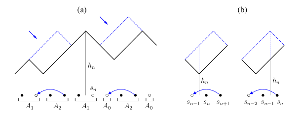
Figure 1: (a) Schematic view of a dimer-growing BCSOS interface (formed by slopes $s_{n}\equiv h_{n+1}-h_{n}=\pm 1$) and its equivalent driven lattice gas of reconstituting particles. At each step of the former, a dimer aggregation on local minima corresponds in the latter to an exchange of $A_{2}$- ‘particles’ with either of the $A_{0}$ or $A_{1}$ ‘vacancies’ referred to in the text. Note that under $A_{1}A_{2}\to A_{2}A_{1}$ exchanges the indentity of $A_{2}$- dimers is not preserved. (b) Sublattice currents contributing to the growth velocity of $h_{n}$ as discussed through Eqs. (5)-(8).

At each successful step $k$-contiguous locations increase their heights in two unit lengths, the rates of deposition being uniform and set equal to one per unit time. Thus, we see that the distance between a minimum and its nearest right maximum is preserved modulo $k$, in turn bringing about correlated movements and many-sector decomposition of the interface walks.

The partitioning of the phase space of these paths can be understood with the aid of a mapping into a modification of the asymmetric simple exclusion process (ASEP) Ligget , hereafter referred to as $k$-ASEP Barma2 . It consists of driven hard-core extended particles occupying $k$ consecutive sites while moving leftward by one site (e.g. $\circ\bullet\bullet\rightarrow\bullet\bullet\circ$ say for dimers). Now, following Ref. Plischke , if we think of these 0,1 occupancies as stemming from Ising variables associated with the slopes $s_{n}=h_{n+1}-h_{n}$ of the interface (cf. Fig. 1), it is then clear that up to an immaterial constant its heights are obtained as $h_{n}=\sum_{j=1}^{n}s_{j}$. On the other hand since the interface is grown only out of $k$-mers, note that in the $k$-ASEP representation neither monomers nor groups or fragments of $j$-adjacent particles can move explicitly if $j<k$, although they are allowed to in a series of steps. For instance, in the sequence

$$0\,\underbracket{1.\,.1}_{j}\,0\,\underbracket{1\dots 1}_{k}\;\rightarrow\;0\,\underbracket{1\dots 1}_{j}\,\underbracket{1.\,.1}_{k}\,0\;\rightarrow\;\underbracket{1\dots 1}_{k}\,0\,\underbracket{1.\,.1}_{j}\,0\,,$$ (2)

the initial leftmost group of $j$ particles can hop $k$-sites to the right provided that $k$-mers can dissociate and reconstitute, so they do not maintain their indentity throughout (except in the absence fragments; see below). In turn following Ref. Barma3 , these processes can also be interpreted as $k$-mer ‘particles’ $A_{k}$ moving through a set of $k$ composite characters or ‘vacancies’ constructed as

$$A_{0} \equiv 0\,,$$

$$A_{1} \equiv {}_{{}_{\hskip-11.09654pt\vdots}}\;\;\,1\,0\,,$$ (3)

$$A_{j} \equiv \underbracket{1\dots 1}_{j}\,0\;,\;\;1<j<k\,.$$

The movements and recompositions of $k$-mers can then be thought of as character exchanges of the form $A_{j}\,A_{k}\rightarrow A_{k}\,A_{j}$, the $k$-mer identity being preserved only by $A_{0}$, whereas exchanges not involving $A_{k}$ remain disabled, (i.e. $A_{i}\,A_{j}$ do not swap their positions if $i,j\neq k\,$). In this notation, for example the steps referred to in Eq. (2) now become $A_{0}\,A_{j}\,A_{k}\rightarrow A_{0}\,A_{k}\,A_{j}\rightarrow A_{k}\,A_{0}\,A_{j}$. But the key issue to point out here is that the $A_{0},A_{1},\cdots,A_{k-1}$ characters define a sequence or irreducible string (IS) whose ordering (set by the initial conditions) is conserved throughout all subsequent times. Thus, the invariant IS of a given sector of motion just refers to the succession of vacancy types obtained after deleting all $k$-mers or ‘reducible’ characters appearing in any configuration of that sector. In other words, all states linked by the $k$-ASEP dynamics have the same IS.

Effective ASEP.— Before evaluating the number of conservation laws yielded by this nonlocal construction, let us first remark that any state of these driven and reconstituting gases can be mapped to an equivalent ASEP configuration defined on a smaller effective lattice Barma3 . More specifically, denoting by $N_{j}$ the number of $A_{j}$ characters (preserved throughout), and therefore given an IS sector of length ${\cal L}=\sum_{j\neq k}(j+1)N_{j}$, it is then clear that the $k$-ASEP dynamics amounts to an ASEP one with $N_{k}=(L-{\cal L})/k$ hard-core particles note2 driven through $N=\sum_{j}N_{j}$ sites; the effective density of such particles then being

$$\rho_{{}_{ASEP}}^{-1}=1+\frac{k}{L-\cal L}\,\sum_{j\neq k}N_{j}\,.$$ (4)

Thus, tagging the vacancies of a generic ASEP configuration in the same order as that appearing for the irreducible characters of a particular sector of motion, one can readily find the corresponding $k$-ASEP state just replacing the $n$-th ASEP vacancy by the $n$-th IS character, whilst substituting every ASEP particle in between by $k$-consecutive occupied sites. For instance, in an IS sector beginning as $A_{1},A_{0},A_{0},A_{1},\cdots$, say for dimers, the ASEP configuration $1\,0\,1\,0\,0\,1\,0\,\cdots$ will be mapped to $(11)(10)(11)(0)(0)(11)(10)\cdots$ $k$-ASEP occupancies. Now, recalling that under PBC the ASEP has a uniform steady state measure Ligget (i.e. all configurations are equally weighted), evidently it follows that this mapping will enable us to sample the steady state of generic IS sectors without explicitly evolving the $k$-ASEP in time.

Growth rates.— Under PBC the effective ASEP also allows for the evaluation of growth velocities. Since the original chain can be partitioned into $k$-sublattices $\Lambda_{1},\cdots,\Lambda_{k}$ note2 , each $k$-mer covers one of their $L/k$ locations and so the $k$-ASEP dynamics preserves the monomer density per sublattice (also determined by the initial conditions). In turn, this defines $k$-stationary sublattice currents (eventually equivalent depending on the IS considered), given by

$$J_{\alpha}=\big{\langle}\left(1-n_{i-k}\right)\;n_{i-k+1}\cdots\,n_{i}\,\big{\rangle}\,,\;\forall\,i\in\Lambda_{\alpha}\;,\;\alpha=1,\cdots,k\,,$$ (5)

where the $n$’s denote sets of $k$-ASEP occupation numbers, cf. Fig. 1(b). But in view of the above mapping, each of these former corresponds to a set of $\{\nu_{1},\cdots,\nu_{N}\}$ occupations in the effective ASEP, so in particular it must hold that

$$\sum_{\alpha=1}^{k}\,\sum_{\;i\in\Lambda_{\alpha}}\left(1-n_{i-k}\right)\;n_{i-k+1}\cdots\,n_{i}=\sum_{j=1}^{N}\,\left(1-\nu_{j}\right)\,\nu_{j+1}\,.$$ (6)

Here, the left hand side just counts the number of feasible movements in a given $k$-ASEP configuration which in turn must coincide with those counted by the right hand terms in the equivalent ASEP state. At this point it is worth mentioning that despite that for PBC all $k$-ASEP configurations are equally likely, the correlators involved in the sublattice currents (5) are not factorizable Barma2 ; Barma3 . However, since for large $N$ the ASEP correlators do decouple under PBC Ligget , it is then clear that as a result of Eq. (6) the net sum of these currents amounts to

$$\sum_{\alpha=1}^{k}J_{\alpha}\simeq\frac{kN}{L}\;\rho_{{}_{{}_{\!\!ASEP}}}\left(1-\rho_{{}_{{}_{\!\!ASEP}}}\right)\,.$$ (7)

So, when it comes to the growth rates of the interface representation, from Fig. 1(b) we can readily identify them with the contribution of all currents crossing a given height location, i.e. ${\rm v}_{k}=\sum_{\alpha}J_{\alpha}$, each contribution here being associated with probabilities of mutually exclusive events wherein the height can grow. As for the density of ASEP particles in (7), further to Eq. (4) note that PBC also impose $\sum_{n}s_{n}\equiv 0$  (i.e. $h_{L}-h_{1}=\pm 1$), for which the vacancy numbers there involved are constrained to add up to $L/2$ note2 . Therefore, we are left with a chain of $N=L/2+(L-{\cal L})/k$ ASEP sites and $\rho_{{}_{\!ASEP}}^{-1}=1+k/[\,2\,(1-{\cal L}/L)\,]$, so the growth velocity (7) simply reduces to

$${\rm v}_{k}({\cal L})=\left(\frac{\,2\,}{k}+\frac{1\,}{1-{\cal L}/L\,}\right)^{\!\!-1}.$$ (8)

As expected, so long as the $k$-ASEP dynamics is not fully jammed, i.e. ${\cal L}<L$, the interface can grow with finite rates, in turn being independent of the vacancy ordering in the string or sector considered.

Exponential growth of invariant sectors.— From the above discussion it follows that the periodicity of these interfaces constrains each string to include $L/2$ 0’s, i.e. $L/2$ charcaters $A_{i}\neq A_{k}$, and ${\cal L}-L/2$  1’s. Moreover, the IS lengths $\mathcal{L}$ are restricted to belong to the set ${\cal S}_{L}^{{}^{(k)}}=\left\{L,L-k,L-2k,\,\cdots,L/2\right\}$, since an integer number of $k$-mers should be required to complete the total length $L$. More specifically, in terms of the vacancy numbers this reads

$$\sum_{i=0}^{k-1}\,N_{i}=L/2,\;\;\;\sum_{i=1}^{k-1}(i+1)\,N_{i}\in\mathcal{S}_{L}^{(k)}\,,\vspace{-0.1cm}$$ (9)

and thereby the total number of irreducible sequences can be expressed as

$$\mathcal{I}_{k}(L)=\sum_{\{N_{i}\}}\,\!\!^{{}^{\prime}}M(\{N_{i}\})\,.$$ (10)

Here, the primed sum is a mnemonic device reminding us that the sum only goes over the sets $\{N_{i}\}$ complying with (9), and $M(\{N_{i}\})$ denotes their “multiplicities”, i.e. the number of different orderings of the irreducible characters of the string. For PBC these orderings are counted up to cyclic permutations of those characters, so that they are given by the “circular multinomial coefficient” Riordan

$$M(\{N_{i}\}) =\frac{1}{N_{0}+N_{1}+\cdots+N_{k-1}}\sum_{d|\gcd(\{N_{i}\})}\varphi(d)\binom{\frac{N_{0}+\dots+N_{k-1}}{d}}{\tfrac{N_{0}}{d}\quad\cdots\quad\tfrac{N_{k-1}}{d}}$$

$$=\frac{2}{L}\sum_{d|\gcd(\{N_{i}\})}\varphi(d)\binom{\tfrac{L}{2d}}{\tfrac{N_{0}}{d}\quad\cdots\quad\tfrac{N_{k-1}}{d}}\,,$$ (11)

where $\varphi(n)$ is the Euler’s totient function Abramowitz , and in the second line we used the first constraint of Eq. (9).

For $k=2$, we can perform the sum in (10) to see that

$$\mathcal{I}_{2}(L)=\frac{1}{L}\,\sum_{d\big{|}\tfrac{L}{2}}\varphi\left(\tfrac{L}{d}\right)2^{d}\,,$$ (12)

so that in the $L\to\infty$ limit the sum over the divisors of $L/2$ is always dominated by the term $d=L/2$ and the number of invariant sectors grows as $2^{L/2}L^{-1}$. For $k\geq 3$ it is harder to do an exact calculation, but we can find numerically the rates at which these sectors grow. These are listed in Table 1 where it is clear that $\mathcal{I}_{k}(L)\simeq 2^{L}$ as $k\to\infty$, as was to be expected.

$k$	2	3	4	5	6	7
$\mathcal{I}_{k}^{1\!/\!L}\!(L)\propto$	1.41421	1.73205	1.8999	1.958	1.981	1.991

Table 1: Growth rates for the total number of sectors of motion [ Eq. (10) ] under PBC.

We can also obtain a lower bound $\mathcal{I}^{*}_{k}(L)$ for $\mathcal{I}_{k}(L)$ by noting that

$$M(\{N_{i}\})\geq M^{*}(\{N_{i}\})\equiv\frac{1}{N_{0}+N_{1}+\cdots+N_{k-1}}\binom{N_{0}+N_{1}+\cdots+N_{k-1}}{N_{0}\quad N_{1}\quad\cdots\quad N_{k-1}}\,,$$ (13)

so that using (9) we have

$$\mathcal{I}_{k}(L)\geq\mathcal{I}^{*}_{k}(L)\equiv\frac{2}{L}\sum_{\{N_{i}\}}\,\!\!^{{}^{\prime}}\binom{L/2}{N_{0}\quad\cdots\quad N_{k-1}}\,.$$ (14)

For $k=2$ this bound gives

$$\mathcal{I}_{2}^{*}(L)=\frac{2}{L}\,\sum_{i=0}^{L/4}\binom{L/2}{2i}=\frac{2^{L/2}}{L}\,,$$ (15)

so it correctly captures the rate we had already found. For $k=3$ one may show that $\mathcal{I}_{3}^{*}(L)$ satisfies the recursion

$$\frac{L}{2}\,\mathcal{I}_{3}^{*}(L)=\left(\,\tfrac{5}{2}L-4\right)\,\mathcal{I}_{3}^{*}(L-2)-3\left(\tfrac{1}{2}L-2\right)\left[\,\mathcal{I}_{3}^{*}(L-4)+3\,\mathcal{I}_{3}^{*}(L-6)\,\right]\,,$$ (16)

so that for large $L$ the total number of invariant sectors is at least

$$\mathcal{I}_{3}^{*}(L)\simeq\frac{3^{\tfrac{L}{2}-1}}{2}\left(1+3\sqrt{\tfrac{3}{2\pi L}}\right)\,.$$ (17)

Once more, the bound given by $\mathcal{I}_{3}^{*}(L)$ seems to be tight in the $L\to\infty$ limit, and we can check numerically that this is also the case for $k>3$.

Roughening exponents.— Armed with the effective ASEP correspondence referred to earlier on, we extensively sampled the stationary configurations of both dimer and trimer interfaces in some periodic IS sectors. These are specified in Table 2 along with their growth velocities [ Eq. (8) ], and sublattice densities (arising from simple stoichiometric considerations). Each state was prepared by random deposition of $N_{k}=(L-{\cal L})/k$ ‘monomers’ on a ring of $L/2+N_{k}$ effective sites [ cf. Eq. (9) ] which, depending on their locations and occupancies, were then transformed to $k$-ASEP configurations according to the mapping discussed before. This enabled us to implement a sampling algorithm with a number of operations bounded as ${\cal O}[\,{\rm N}_{s}(L/2+N_{k})\,]$, while using a number of samples ${\rm N}_{s}$ such that ${\rm N}_{s}\sim 10^{11}/L$ and substrates sizes of up to $10^{6}$ locations, thus significantly reducing the scatter of averaged data.

$k$	IS sector	Density	Growth rate	$\langle\,W^{2}\rangle/L$	$\langle\,{\rm h_{m}}\,\rangle/L^{1/2}$
	$[A_{{}_{0}}]^{L/2}$	1/2	1/3	0.125(1)	0.766(2)
dimers	$[A_{{}_{1}}A_{{}_{0}}^{2}]^{L/6}$	$\begin{cases}\rho_{1}=2/3\vspace{0.125cm}\cr\rho_{2}=1/3\end{cases}$	1/4	0.074(1)	0.583(2)
	$[A_{{}_{1}}A_{{}_{0}}]^{L/4}$	1/2	1/5	0.052(1)	0.494(2)
	$[A_{{}_{0}}]^{L/2}$	1/2	3/8	0.166(1)	0.881(1)
trimers	$[A_{{}_{2}}A_{{}_{0}}^{3}]^{L/8}$	$\begin{cases}\rho_{1}=\rho_{2}=5/8\vspace{0.125cm}\cr\rho_{3}=1/4\end{cases}$	3/14	0.073(1)	0.584(1)
	$[A_{{}_{2}}A_{{}_{1}}A_{{}_{0}}^{3}]^{L/10}$	1/2	3/17	0.056(2)	0.515(2)

Table 2: Sublattice densities, growth velocities, and amplitudes of average widths and maximal heights for dimers and trimers in the irreducible strings studied in the main panels of Figs. 2 and 3. Sectors of motion are formed by concatenating the string characters of Eq. (3), e.g. $[A_{1}A_{0}^{2}]^{L/6}$ just repeats $[(10)(0)(0)]\;L/6$ times (so, ${\cal L}/L=2/3$), etc.

In Fig. 2(a) we exhibit the growth of the stationary widths (1) spread over several decades of substrate lengths. As anticipated in the introductory paragraphs, despite the correlated movements and partitioning of the interface paths, all cases evidence the appearance of diffusive roughening exponents typical of monomer growing interfaces either in the KPZ or EW classes Meakin ; KPZ ; Edwards . For display purposes, here the width of each dynamic sector was rescaled by the corresponding amplitudes of Table 2, in turn decreasing with their growth velocities (as they should).

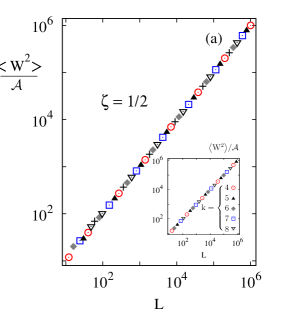
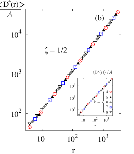
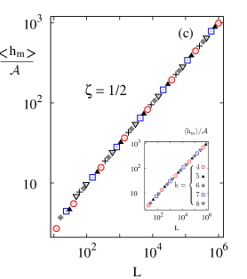
Figure 2: (a) Finite-size growth of average widths, (b) height difference correlation functions ($L=4.2\times 10^{5}$), and (c) growth of average maximum heights (measured with respect to spatially averaged ones), for various string sectors. In main panels, circles, squares, and rhomboids stand respectively for the first three sectors of Table 2 ($k=2$), whereas its following ones correspond to triangles, downwards triangles, and plus signs ($k=3$). Insets denote in turn cases of null string sectors with $k\geq 4$. All data in main panels (insets) were normalized by $\cal A$- amplitudes given in the rightmost columns of Table 2 (Table 3), and are consistent with a common roughening exponent $\zeta=1/2$.

Alongside Eq. (1) we also examined the stationary height difference correlation functions for which a similar scaling behavior involving the same roughening exponent is also expected to hold at distances $|r|\ll L$, that is Meakin ; Family

$$\langle\,D_{{}_{\!\!L}}^{2}(r)\,\rangle=\frac{1}{L}\,\sum_{n}\left\langle\big{[}\,h_{n+r}-\,h_{n}\,\big{]}^{2}\right\rangle\propto|r|^{2\zeta}.$$ (18)

In fact, this is corroborated in Fig. 2(b) where these correlations turn out to scale linearly with the height separation for all IS sectors considered. As before, the results were made to collapse by the normalization amplitudes used for the average widths of Fig. 2(a), as would be expected on the basis of the identity $\lim_{{}_{{}_{\!\!\!\!\!\!\!\!\!\!\!r\to\infty}}}\lim_{{}_{{}_{\!\!\!\!\!\!\!\!\!\!\!L\to\infty}}}\!\langle D_{{}_{\!\!L}}^{2}(r)\rangle=\lim_{{}_{{}_{\!\!\!\!\!\!\!\!\!\!\!L\to\infty}}}\!\!2\,\langle W_{{}_{\!\!L}}^{2}\rangle$.

Another stationary quantity of interest whereby the roughening exponent can also be tested concerns the average maximal height $\langle{\rm h_{m}}\rangle_{\!{}_{L}}$ measured with respect to the spatially averaged height of each interface realization, namely

$$\left\langle\,{\rm h_{m}}\right\rangle_{\!{}_{L}}=\left\langle\,\max\left\{h_{1}-\bar{h},\,\cdots\,,h_{L}-\bar{h}\right\}\,\right\rangle\propto L^{\zeta}\,,$$ (19)

thus capturing possible extreme fluctuations that neither the average width nor the height difference correlations are able to measure. The scaling of this quantity along with its stationary probability distribution (see below), have been investigated numerically Shapir in discrete 1D growth models belonging to the EW class, as well as analytically Majumdar applying path integral methods to both 1D EW and KPZ equations. In agreement with those studies, here also the correlated and partitioned paths described by our $k$-mer interfaces recover the diffusive scaling of $\langle{\rm h_{m}}\rangle_{\!{}_{L}}$ with the substrate size in all IS sectors of Table 2. This is shown in Fig. 2(c) for a wide range of $L$ sizes after normalizing the data by the amplitudes of each sector. As might be presumed, these latter still decrease with their growth velocities and in all cases are quite larger than the corresponding width amplitudes (cf. Table 2).

To complement the diffusive picture discussed so far, we also estimated the roughening exponents of Eqs. (1), (18), and (19) in nonreconstituting $[A_{0}]^{L/2}$ sectors of interfaces virtually grown out of several other $k$-mer values. This is displayed in the insets of Figs. 2(a), 2(b), and 2(c) where, just as in main panels, a $1/2$ scaling exponent can also be read off from their slopes. The normalizing amplitudes that produce the data collapse are quoted in Table 3, and in parallel with the growth velocities $k/[2(k+1)]$ these come out increasing monotonically with $k$, as was to be expected.

$k$	$\langle\,W^{2}\rangle/L$	$\langle\,{\rm h_{m}}\,\rangle/L^{1/2}$
4	0.208(1)	0.987(1)
5	0.250(1)	1.083(2)
6	0.292(1)	1.162(5)
7	0.334(1)	1.245(9)
8	0.375(1)	1.322(4)

Table 3: Amplitudes of average widths and maximal heights for the null string sectors considered in the insets of Fig. 2.

Scaling distributions.— Turning to a more detailed level of description, next we focus our attention on the probabilities $P\left({\rm h_{m}}\right),P\left(w^{2}\right)$ of stationary realizations of both widths and maximal heights. Since their averages diverge in the thermodynamic limit, it has been argued on general grounds Zia ; Shapir ; Majumdar ; Schehr ; Racz ; Parisi that for large substrate sizes these probability distributions should scale as

$$P_{\!\!{}_{L}}\left(w^{2}\right)\simeq\frac{1}{\langle\,W_{\!\!{}_{L}}^{2}\,\rangle}\,\Phi\left(\frac{w^{2}}{\langle\,W_{\!\!{}_{L}}^{2}\,\rangle}\right)\,,\;\;\;P_{\!\!{}_{L}}\left({\rm h_{m}}\right)\simeq\frac{1}{\langle\,{\rm h_{m}}\,\rangle_{\!{}_{L}}}\,F\left(\frac{{\rm h_{m}}}{\langle\,{\rm h_{m}}\,\rangle_{\!{}_{L}}}\right)\,,$$ (20)

where $\Phi(x)$ and $F(x)$ are characteristic scaling functions of a variety of solid-on-solid growth models Zia ; Schehr , although their dependence on boundary conditions is also a relevant issue Majumdar ; Schehr ; Halpin-Healy .

In particular under PBC, where the $k$-ASEP mapping has so far been applied, these scaling functions were evaluated exactly in 1D Brownian interfaces, thus enabling us to go a step further in the characterization of our $k$-mer models. This we do in Figs. 3(a) and 3(b) where the scaled probability distributions of $w^{2}$ and ${\rm h_{m}}$ in all IS sectors of Table 2 are compared with the analytical expressions of $\Phi$ and $F$ obtained respectively in Refs. Zia and Majumdar , namely

$$\Phi(x) = \frac{\pi^{2}}{3}\,\sum_{n\geq 1}\,(-1)^{n-1}\,n^{2}\,\exp\left(-\frac{\pi^{2}}{6}n^{2}x\right)\,,$$ (21a)

$$F(x) = \frac{2\,\sqrt{6}}{x^{10/3}}\,\sum_{n\geq 1}\,b_{n}^{2/3}\,\exp\left(-\frac{b_{n}}{x^{2}}\right)\,U\!\left(-\frac{5}{6}\,,\,\frac{4}{3}\,,\,\frac{b_{n}}{x^{2}}\,\right)\,.$$ (21b)

Here $U(x_{1},x_{2},x_{3})$ denotes the confluent hypergeometric function Abramowitz , whereas $b_{n}\equiv 2\left(|a_{n}|/3\right)^{3}$ involves the magnitudes of the Airy function zeros ($a_{n}$) on the negative real axis Majumdar ; Abramowitz . Using substrates in the range of $10^{4}\,-\,10^{5}$ heights, the probability densities were reconstructed by means of the convolution of $10^{7}$ data points (in turn derived from independent $k$-ASEP samples), with a Gaussian kernel whose bandwidth was determined by Silverman’s method Silverman .

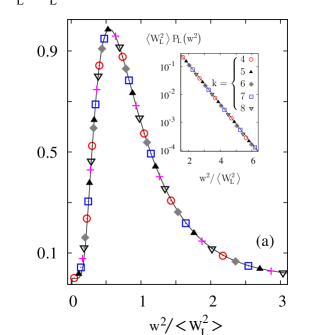
Figure 3: Scaling of (a) width distributions, and (b) maximal height distributions for the $k$-mer sectors of Table 2 using the symbols of Fig. 2. Here, these stand for sizes $L=3\times 10^{4}$ (circles), $6\times 10^{4}$ (rhomboids), $10^{5}$ (squares), $2.4\times 10^{4}$ (triangles), $4.8\times 10^{4}$ (plus signs), and $9\times 10^{4}$ (downwards triangles). For comparison, in (a) and (b) solid lines correspond respectively to the exact scaling functions referred to in Eq. (21a) (Ref. Zia ), and Eq. (21b) (Ref. Majumdar ). The insets exhibit the tails of those scaling distributions which also follow our data in the null string sectors of $k=4,\,5,\,6,\,7,\,8$ with $L=(\,3.6,\,4.2,\,3.3,\,2.8,\,4\,)\times\!10^{4}$ respectively.

In all sectors considered the data collapse is in excellent agreement with the scaling distributions (21a) and (21b). Here, note that there are no parameters to fit these stationary functions and that no scaling properties neither for $\langle\,W_{\!\!{}_{L}}^{2}\,\rangle$ nor $\left\langle\,{\rm h_{m}}\right\rangle_{\!{}_{L}}$ have been used, the only approximation being the finite size of the substrates. The data collapse towards the tails of these distributions is also corroborated in the insets of Figs. 3(a) and 3(b) where other $k$-mer values are examined in nonreconstructing $[A_{0}]^{L/2}$ sectors. For large realizations of $w^{2}$ and ${\rm h}_{m}$ the resulting slopes of the semilogarithmic plots displayed there in fact coincide with those derived from the asymptotic behavior of $\Phi$ and $F$, decaying respectively as $\exp(-\frac{\pi^{2}}{6}x)$ and $\exp(-6\,x^{2})$ (cf. Refs. Zia ; Majumdar ).

Further to periodic strings, we also considered disordered IS sectors obtained from the former by random permutations of their characters. It is worth mentioning that preliminary results also indicate that the above scaling distributions continue to stand as generic features of that disordered situation.

Faceting.— Finally however, and in marked contrast with that robustness, let us comment on string sectors that include long concatenations of identical vacancy types, such as those considered in Fig. 4. When the length of these domains becomes of the order of the substrate size, it turns out that the implicit assumption of a well-defined average orientation of the interface (parallel to the substrate) is no longer consistent. Instead, a faceted structure with large scale slopes emerges. This is illustrated by the snapshots shown in the insets of Figs. 4(a) and 4(b), each of their facets stemming from different character domains along their strings. Moreover, as suggested by the width distributions displayed in main panels, statistical fluctuations in these structures are progressively suppressed as $L$ increases.

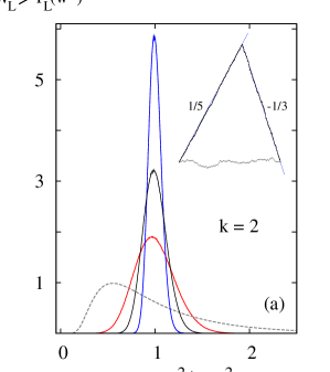
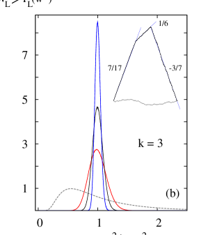
Figure 4: Width distributions of faceting sectors (a) $[A_{1}]^{L/4}[A_{0}]^{L/4}$ (${\cal L}/L=3/4$), and (b) $[A_{2}]^{L/10}[A_{1}]^{L/10}[A_{0}]^{3L/10}$ (${\cal L}/L=4/5$) for $L=10^{4},3\times 10^{3},$ and $10^{3}$ (topmost solid lines in downward direction). In contrast to roughening sectors (lowermost universal distribution), fluctuations around average widths become negligible as $L$ increases. Snapshots of the resulting interfaces ($L=10^{4}$) are displayed by the insets. The slopes of their facets (indicated by dashed lines) are evaluated in the text. For comparison, snapshots of the roughening sectors $[A_{1}\,A_{0}]^{L/4}$, and $[A_{2}\,A_{1}\,A_{0}^{3}\,]^{L/10}\!$ are also exhibited in (a) and (b) respectively.

In that latter respect we can assume a uniform density of effective ASEP particles for most interface realizations so as to readily estimate the slope of each facet. Thus, if there are $n$ characters in a given domain, clearly the average number of $k$-mers amid them should be $n(\frac{L-{\cal L}}{k})/\sum_{i=0}^{k-1}\,N_{i}=\frac{2n}{k}(1-{\cal L}/L)$ [ see PBC constraints of Eq. (9) ]. Since each $A_{j}$ involves $j$ monomers and a vacancy, then the average length of such set ($A_{j}$-characters and $k$-mers combined) must comprehend $n(j+1)+2n(1-{\cal L}/L)$ sites of the substrate ($n\leq N_{j}$). Analogously, the average height difference along that set becomes $n(j-1)+2n(1-{\cal L}/L)$. Thereby, we are left with slopes $1-\left(\frac{j+3}{2}-\frac{\cal L}{L}\right)^{-1}$ that closely follow those arising from the $A_{j}$-domains considered in the strings of Fig. 4. Note that these average slopes can vanish only in nonreconstituting $[A_{0}]^{L/2}$ sectors but, as seen above, in such cases the usual roughening behavior is restored.

To summarize, we have studied stationary aspects of 1D interfaces formed by deposition of extended particles within the context of a mapping to a process of driven and reconstituting $k$-mers Barma2 ; Barma3 . This enabled us to sample the steady state without having to explicitly evolve the system in time, and, as a result, a rich statistical analysis of both stationary width and maximal height distributions was attained at large substrate scales. For clarity of presentation the models were defined as totally asymmetric, although extensions using partially asymmetric or even symmetric versions subject to PBC would make no difference to the stationary distributions.

The notion of irreducible string played a key role in the understanding of the behavior of these interfaces as it encodes nonlocal conserved quantities that partition the growth dynamics into an exponential number of disjoint sectors of motion with specific growth velocities. Owing to the spatial extension of the deposited $k$-mers, the path phase space of these sectors actually corresponds to sets of correlated random walks. However, in view of the diffusive roughening exponents obtained for several IS sectors, these walks turn out to follow the typical root mean square displacement associated with the stationary roughness of the 1D KPZ and EW classes. Finally, at the more demanding level of width and maximal height probability distributions, all roughening sectors considered also reproduced the exact scaling functions Zia ; Majumdar of those universality classes. Whether these numerical findings could be explained theoretically remains an open issue which, in turn, should also account for the existence of faceting sectors.

References

- (1) For comprehensive reviews and literature list consult P. Meakin, Fractals, Scaling and Growth Far from Equilibrium (Cambridge University Press, Cambridge 1998); P. Meakin, Phys. Rep. 235, 189 (1993); J. Krug, Adv. Phys. 46, 139 (1997); T. Halpin-Healy and Y.-C. Zhang, Phys. Rep. 254, 215 (1995); A.-L Barbási and H. E. Stanley, Fractal Concepts in Surface Growth (Cambridge University Press, 1995); C. Misbah and Y. Saito, Rev. Mod. Phys. 82, 981 (2010).
- (2) G. Ódor, Universality in Nonequilibrium Lattice Systems. Theoretical Foundations, Chap. 7 (World Scientific, Singapore, 2008); G. Ódor Rev. Mod. Phys. 76, 663 (2004).
- (3) M. Henkel, H. Hinrichsen, and S. Lübeck, Non-Equilibrium Phase Transitions, Vol. 1 (Springer, Dordrecht, 2008), Chaps. 3–5
- (4) M. Kardar, G. Parisi, and Y.-C. Zhang, Phys. Rev. Lett. 56, 889 (1986).
- (5) F. Family and T. Vicsek, J. Phys. A 18, L75 (1985); J. Kertész and T. Vicsek in Fractals in Science, edited by A. Bunde and S. Havlin (Springer, Berlin, 1994).
- (6) S. F. Edwards and D. R. Wilkinson, Proc. R. Soc. London, Ser. A 381, 17 (1982). Let us recall that in dimensions, both EW and KPZ equations share the same steady-state measure.
- (7) J. D. Noh, H. Park, and M. den Nijs, Phys. Rev. Lett. 84, 3891 (2000); J. D. Noh, H. Park, D. Kim, and M. den Nijs, Phys. Rev. E 64, 046131 (2001).
- (8) Y. Kim, S. Y. Yoon, and H. Park, Phys. Rev. E 66, 040602(R) (2002); Y. Kim and S. Y. Yoon, ibid. 69, 027101 (2004).
- (9) H. Hinrichsen and G. Ódor, Phys. Rev. Lett. 82, 1205 (1999); Phys. Rev. E 60, 3842 (1999).
- (10) M. Arlego and M. D. Grynberg, Phys. Rev. E 88, 052408 (2013); M. D. Grynberg, J. Stat. Phys. 103, 395 (2001).
- (11) These matter in the roughening of vicinal surfaces, see D.-S. Lee and M. den Nijs, Phys. Rev. E 65, 026104 (2002); as well as in the growth of organic thin films, consult S. Zorba, Y. Shapir, and Y. Gao, Phys. Rev. B 74, 245410 (2006).
- (12) M. Barma and D. Dhar, Phys. Rev. Lett. 73, 2135 (1994); D. Dhar and M. Barma, Pramana–J. Phys. 41, L193 (1993).
- (13) G. Foltin, K. Oerding, Z. Rácz, R. L. Workman, and R. K. P. Zia, Phys. Rev. E 50, R639 (1994).
- (14) S. Raychaudhuri, M. Cranston, C. Przybyla, and Y. Shapir, Phys. Rev. Lett. 87, 136101 (2001).
- (15) S. N. Majumdar and A. Comtet, Phys. Rev. Lett.92, 225501 (2004); J. Stat. Phys. 119, 777 (2005).
- (16) G. Schehr and S. N. Majumdar, Phys. Rev. E 73, 056103 (2006).
- (17) M. Plischke, Z. Racz, and D. Liu, Phys. Rev. B 35, 3485 (1987).
- (18) T. M. Ligget, Interacting Particle Systems (Springer-Verlag, New York, 1985); B. Derrida and M. R. Evans in Nonequilibrium Statistical Mechanics in One Dimension, edited by V. Privman (Cambridge University Press, UK, 1997); G. M. Schütz, in Phase Transitions and Critical Phenomena, edited by C. Domb and J. L. Lebowitz, Vol. 19 (Academic Press, London, 2001); J. de Gier and F. H. L. Essler, J. Stat. Mech. P12011, (2006).
- (19) S. Gupta, M. Barma, U. Basu, and P. K. Mohanty, Phys. Rev. E 84, 041101 (2011).
- (20) G. I. Menon, M. Barma, and D. Dhar, J. Stat. Phys. 86, 1237 (1997); M. Barma, M. D. Grynberg, and R. B. Stinchcombe, J. Phys.: Condens. Matter 19, 065112 (2007).
- (21) For simplicity, hereafter substrate sizes and string lengths are chosen such that , and .
- (22) J. Riordan, Introduction to Combinatorial Analysis, Chap. 6 (Dover Publications, New York, 2002).
- (23) Handbook of Mathematical Functions, edited by M. Abramowitz and I. A. Stegun (Dover Publications, New York, 1973).
- (24) M. Plischke, Z. Rácz, and R. K. P. Zia, Phys. Rev. E 50, 3589 (1994); Z. Rácz and M. Plischke, Phys. Rev. E 50, 3530 (1994); T. Antal and Z. Rácz, Phys. Rev. E 54, 2256 (1996).
- (25) E. Marinari, A. Pagnani, G. Parisi, and Z. Rácz, Phys. Rev. E 65, 026136 (2002); A. Rosso, W. Krauth, P. Le Doussal, J. Vannimenus, and K. J. Wiese, Phys. Rev. E 68, 036128 (2003); F. D. A. Aarão Reis, Phys. Rev. E 72, 032601 (2005).
- (26) The role of other boundary conditions on scaling distributions in several KPZ experimental and numerical contexts have been reviewed by T. Halpin-Healy and K. A. Takeuchi, J. Stat. Phys. 160, 794 (2015); Secs. 3.1, 3.2, and references therein.
- (27) B. W. Silverman, Density Estimation for Statistics and Data Analysis (Chapman and Hall, London, 1986).