First measurement of the ¹⁴N/¹⁵N ratio in the analogue of the Sun progenitor OMC-2 FIR4

Abstract

We present a complete census of the ¹⁴N/¹⁵N isotopic ratio in the most abundant N-bearing molecules towards the cold envelope of the protocluster OMC-2 FIR4, the best known Sun progenitor. To this scope, we analysed the unbiased spectral survey obtained with the IRAM-30m telescope at 3mm, 2mm and 1mm. We detected several lines of CN, HCN, HNC, HC₃N, N₂H⁺, and their respective ¹³C and ¹⁵N isotopologues. The lines relative fluxes are compatible with LTE conditions and moderate line opacities have been corrected via a Population Diagram method or theoretical relative intensity ratios of the hyperfine structures. The five species lead to very similar ¹⁴N/¹⁵N isotopic ratios, without any systematic difference between amine and nitrile bearing species as previously found in other protostellar sources. The weighted average of the ¹⁴N/¹⁵N isotopic ratio is $270\pm 30$. This ¹⁴N/¹⁵N value is remarkably consistent with the [250$-$350] range measured for the local galactic ratio but significantly differs from the ratio measured in comets (around 140). High-angular resolution observations are needed to examine whether this discrepancy is maintained at smaller scales. In addition, using the CN, HCN and HC₃N lines, we derived a ¹²C/¹³C isotopic ratio of $50\pm 5$.

1 Introduction

The Solar System is the result of a long and complex process, several aspects of which still remain a mistery. One of these is the so-called ”anomalous” ¹⁴N/¹⁵N value in the objects of the Solar System (Caselli & Ceccarelli, 2012; Hily-Blant et al., 2013). Based on the solar wind particles (Marty, 2012), the Solar Nebula value is $441\pm 6$. However, ¹⁴N/¹⁵N is 272 in the Earth atmosphere (Marty, 2012), around 140 in comets (Manfroid et al., 2009; Mumma & Charnley, 2011; Shinnaka et al., 2014; Rousselot et al., 2014), and between 5 and 300 in meteorites (Busemann et al., 2006; Bonal et al., 2010; Aléon, 2010). The Solar System primitive objects as well as the terrestrial atmosphere are, hence, enriched of ¹⁵N with respect to the presumed initial value. It has been long known that, similarly to the ¹⁵N enrichment, the D/H ratio in terrestrial water is about ten times larger than in the Solar Nebula and this is very likely due to the conditions in the earliest phases of the Solar System (see e.g. the reviews by  Ceccarelli et al. (2014a) and  Cleeves et al. (2015)). The reason for the ¹⁵N enrichment has, thus, been searched for in the chemical evolution of matter during the first steps of the Solar System formation (e.g. Terzieva & Herbst (2000); Rodgers & Charnley (2008); Wirström et al. (2012); Hily-Blant et al. (2013)).

Several observations in Solar-like star forming regions have been reported in the literature. In prestellar cores, ¹⁴N/¹⁵N varies between 70 and more than 1000 (Ikeda et al. (2002); Gerin et al. (2009); Milam & Charnley (2012); Daniel et al. (2013); Hily-Blant et al. (2013, 2017); Bizzocchi et al. (2013); Taniguchi & Saito (2017)), in Solar-like Class 0 protostars between 150 and 600 (Gerin et al., 2009; Wampfler et al., 2014), and 80$-$160 in protoplanetary disks (Guzmán et al., 2015, 2017).

Whereas the ¹⁴N/¹⁵N values reported in the literature for prestellar cores, protostars, disks and comets have been derived from the observations of half a dozen of different species (CN, HCN, HNC, NH₃, N₂H⁺, cyanopolyynes), it should be noted that, for each of these objects, only a few species were used each time.

Nonetheless, one has to consider that, rather than to the Solar Nebula ¹⁴N/¹⁵N value, these measurements should be compared to the nowadays local interstellar ¹⁴N/¹⁵N ratio of $\sim{300}$, which results from cosmic evolution in the solar neighbourhood (Romano et al. (2017); Hily-Blant et al. (2017) and references therein) and is, apparently by coincidence, very close to the terrestrial atmosphere value.

In order to understand the origin of the Solar System ¹⁵N enrichment, we need to measure it in objects that are as most as possible similar to the Sun progenitor. The so far known best analogue of the Sun progenitor is represented by the source OMC-2 FIR4, in the Orion Molecular Complex at a distance of 420 pc (Menten et al., 2007; Hirota et al., 2007), north of the famous KL object. Several recent observations show that FIR4 is a young protocluster containing several protostars, some of which will eventually become Suns (Shimajiri et al., 2008; López-Sepulcre et al., 2013; Furlan et al., 2014). In addition, OMC-2 FIR4 shows signs of the presence of one or more sources of energetic $\geq 10$ MeV particles, the dose of which is similar to that measured in meteoritic material (Ceccarelli et al., 2014b; Fontani et al., 2017). In this article, we report the first measure of the ¹⁴N/¹⁵N ratio in OMC-2 FIR4, using different molecules: HC₃N, HCN, HNC, CN and N₂H⁺.

2 Observations

We carried out an unbiased spectral survey of OMC-2 FIR4 (PI: Ana López-Sepulcre) in the 1,2 and 3mm bands with the IRAM 30 m telescope. The 3 mm (80.5$-$116.0 GHz) and 2 mm (129.2$-$158.8 GHz) bands were observed between 31 Aug. and 5 Sep. 2011, and on 24 Jun. 2013. The 1 mm (202.5$-$266.0 GHz) range was observed on 10$-$12 Mar. 2012 and on 7 Feb. 2014. The Eight MIxer Receiver (EMIR) has been used, connected to the 195 kHz resolution Fourier Transform Spectrometer (FTS) units. The observations were conducted in wobbler switch mode, with a throw of 120^′′. Pointing and focus measurements were performed regularly. The telescope Half Power Beam Width (HPBW) is 21$-$30.6^′′, 15.5$-$19^′′ and 9$-$12^′′ in the 1,2 and 3mm bands respectively. The package CLASS90 of the GILDAS software collection was used to reduce the data. The uncertainties of calibration are estimated to be lower than 10% at 3 mm and 20% at 2 mm and 1mm. After subtraction of the continuum emission via first-order polynomial fitting, a final spectrum was obtained by stitching the spectra from each scan and frequency setting. The intensity was converted from antenna temperature ($T_{\mathrm{ant}}^{\ast}$) to main beam temperature ($T_{\mathrm{mb}}$) using the beam efficiencies provided at the IRAM web site. The typical rms noise, expressed in $T_{\mathrm{mb}}$ unit, is 4$-$7 mK in the 3mm band, 8$-$10mK in the 2mm band, and 15$-$25mK in the 1mm band.

3 Results

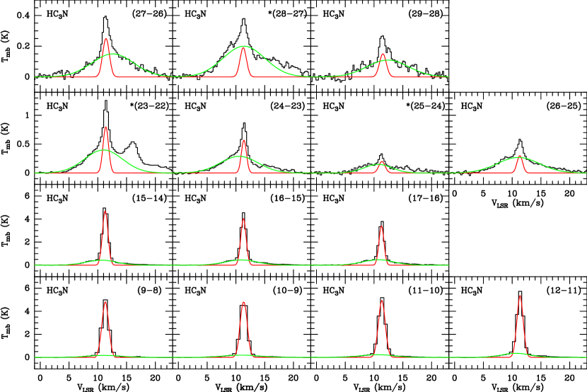
Figure 4: HC₃N observed spectra and two components Gaussian fits to the lines. The temperature scale is main beam temperature. Due to significant overlaping with other emissions or calibration problem, the lines indicated by an asterisc (*) have not been included in our analysis nor reported in Table 1.

In order to derive the ¹⁴N/¹⁵N ratio in OMC-2 FIR4, we have looked for the ¹⁵N-bearing substitutes of all the abundant N-bearing species present in the survey. We have clearly detected and identified the ¹⁵N-isotopologues of five species: HC₃N, HCN, HNC, CN, N₂H⁺, most with more than one line, and tentatively detected one line of H¹³C¹⁵N. In addition, we have also included in our analysis the ¹³C-bearing isotopes of HC₃N, HCN, HNC and CN. A representative sample of these lines is shown in Fig. 1 and all the observed lines are plotted in the Appendix in Figs. 4 to 12.

Figure 1: Representative sample of the observed spectra for the HC₃N, HCN, HNC, N₂H⁺ and CN families. The temperature scale is main beam temperature. Weak lines are indicated by an arrow.

The lines analysis and modeling presented here make use of several tools of the CASSIS package. Gaussian fits have been used to derive the lines integrated intensities (called « fluxes » in the following) and kinematical properties. All lines are well fitted with narrow Gaussian components showing low dispersions in central velocities and linewidths (V_LSR = 11.3 (0.1) km.s^-1, FWHM = 1.4 (0.2) km.s^-1). In addition, the strongest lines also show a slightly displaced broad component (V_LSR = 10.8 (0.3) km.s^-1, FWHM = 6.4 (0.4) km.s^-1 from Gaussian fits), which is not detected in the ¹⁵N-bearing species, except in HC¹⁵N. We have, thus, focussed our work on the narrow component. Figs. 4 to  12 of the Appendix show the Gaussian profiles superimposed to the observed lines. The fluxes reported in Table 1 to Table 4 correspond to the narrow Gaussian components only and the 1 sigma error bars include the fit and the calibration uncertainties.

For HCN, HNC and N₂H⁺, our survey covers only the $(J=1-0)$ transitions of the ¹⁵N-bearing isotopologues. Thus, for these species, to derive of the ¹⁴N/¹⁵N ratio we used the ”flux ratio method” applied to the $(J=1-0)$ transitions of the observed isotopologues. It leads to reliable abundance ratios provided that (i) the $(1-0)$ transitions of the various isotopologues correspond to the same excitation temperature, (ii) the lines are not significantly affected by or can be corrected for opacity effects, (iii) the emission size is the same for the various isotopologues.

For HC₃N and CN, since more than one rotational transition is observed for the ¹⁵N-bearing isotopologues, we could perform a Local Thermal Equilibrium (LTE) modeling to derive the ¹⁴N/¹⁵N abundance ratios, as discussed for each species below.

Whenever possible, we have obtained direct ¹⁴N/¹⁵N measurements. In two cases, HCN and HNC, we have obtained indirect ¹⁴N/¹⁵N derivations from the less abundant isotopologues H¹³CN and HN¹³C, assuming a ¹²C/¹³C ratio.

In all cases, the isotopic ratios that we derive are « beam-averaged » values, at the scale of the largest HPBW of our observations ($\sim 30"$).

3.1 HC₃N

To rely on a coherent set of lines, likely to sample the same gas, we have restricted our analysis to the narrow HC₃N emission, because broad emission from the ¹⁵N and the ¹³C isotopes of HC₃N is not detected in our survey.

Table 1: Integrated intensities from Gaussian fits for HC₃N and its isotopologues.

HC3N				H13CCCN	HC13CCN	HCC13CN	HCCC15N
Transition	Frequency(1)	E${}_{up}^{(1)}$	$\int$Tmbdv	$\int$Tmbdv	$\int$Tmbdv	$\int$Tmbdv	$\int$Tmbdv
$(J^{\prime}-J)$	[MHz]	[K]	[K.km.s-1]	[K.km.s-1]	[K.km.s-1]	[K.km.s-1]	[K.km.s-1]
9$-$8	81881.5	19.6	7.1(0.7)	-	0.11(0.01)	0.16(0.02)	-
10$-$9	90979.0	24.0	7.4(0.7)	0.14(0.01)	0.16(0.02)	0.18(0.02)	0.024(0.007)
11$-$10	100076.4	28.8	7.3(0.7)	0.15(0.02)	0.16(0.02)	0.19(0.02)	0.028(0.006)
12$-$11	109173.6	34.0	7.4(0.7)	0.14(0.01)	0.17(0.02)	0.18(0.02)	0.030(0.010)
13$-$12	114615.0(2)	38.5(2)	-	0.11(0.01)	-	-	-
15$-$14	136464.4	52.4	5.7(1.1)	-	0.10(0.02)	0.13(0.03)	-
16$-$15	145561.0	59.4	4.7(0.9)	0.08(0.02)	0.10(0.02)	0.12(0.02)	-
17$-$16	154657.3	66.8	3.7(0.7)	0.08(0.02)	0.06(0.01)	0.13(0.03)	-
24$-$23	218324.7	130.9	0.6(0.1)	-	-	-	-
26$-$25	236512.8	153.2	0.36(0.07)	-	-	-	-
27$-$26	245606.3	165.0	0.37(0.07)	-	-	-	-
29$-$28	263792.3	189.9	0.22(0.04)	-	-	-	-

• The integrated intensities correspond to the narrow Gaussian components only and the 1 $\sigma$ error bars include the fit and the calibration uncertainties.

• (1) We report in this table only the main isotopologue frequencies and upper level energies, except for the (13$-$12) transition, which falls outside the observed frequency range.

• (2) These values correspond to the H¹³CCCN isotopologue, the only one for which the (13$-$12) transition is covered by our observations.

To derive the column densities of the five species, we have performed a Population Diagram analysis of the lines reported in Table 1, which corrects iteratively for the opacity effects. Large scale maps obtained recently with the IRAM 30m telescope (Jaber Al-Edhari et al., in prep.) show that the cyanopolyyne emission is extended. Thus, no beam dilution correction has been applied. The results of the analysis are shown in Fig. 2.

Figure 2: Population Diagrams for HC₃N and its isotopologues. No beam dilution correction has been applied. The HC₃N data points are shown as black squares when corrected for opacity effects and as empty squares without the opacity correction. The three solid lines correspond to a rotational temperature of 25 K; the dashed line corresponds to an excitation temperature of 50 K.

The HC₃N lines diagram suggests the existence of two components responsible for the narrow emission. After correction of their (moderate) opacity (0.20 to 0.25), the HC₃N lines with upper level energy E_up lower than 130 K are compatible with an LTE excitation at a rotational temperature of 25 K, in agreement with the values derived from the ¹³C isotopes, and a HC₃N column density of 3.3$\times$10¹³ cm^-2. Assuming the same excitation temperature for the HCCC¹⁵N lines, we obtain a column density of 1.2$\times$10¹¹ cm^-2 and a direct determination of the ¹⁴N/¹⁵N abundance ratio of $275\pm 65$. For the three ¹³C-bearing isotopologues of HC₃N, we derive, in the same way, ¹²C/¹³C abundance ratios of $57\pm 7$, $59\pm 11$ and $46\pm 6$. We have checked that an LTE model based on these parameters is perfectly coherent with the non detection of the isotopologues lines at E_up $>$ 70 K.

The HC₃N lines with E_up $>$150 K suggest the existence of a warmer component but its analysis is out of the scope of this article. An extended and detailed modeling of the cyanopolyynes emission in OMC-2 FIR4, relying on a more complete set of data and including the broad emission, is presented in another study (Jaber Al-Edhari et al., in prep.).

3.2 HCN

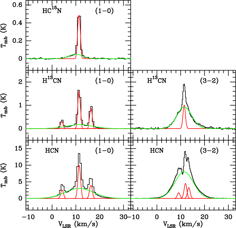
Figure 9: HCN and its isotopologues observed spectra. Two components Gaussian fits to the lines are superimposed to the spectra. The temperature scale is main beam temperature.

The lines of HCN and of its ¹³C- and ¹⁵N- bearing isotopologues show a narrow and a broad emission. We have fitted them by Gaussian profiles (see Table 2 and Fig. 9).

Table 2: Integrated intensities from Gaussian fits for HCN and its isotopologues.

HCN					H13CN	HC15N	H13C15N
Transition	Frequency(2)	E${}_{up}^{(2)}$	Component(3)	$\int$Tmbdv(4)	$\int$Tmbdv(4)	$\int$Tmbdv(4)	$\int$Tmbdv(4)
$(J^{\prime}_{F^{\prime}}-J_{F})$ or $(J^{\prime}-J)$ (1)	[MHz]	[K]		[K.km.s-1]	[K.km.s-1]	[K.km.s-1]	[K.km.s-1]
$1_{1}-0_{1}$	88630.4	4.3	N	8.4(0.9)	1.3(0.1)	-	-
$1_{2}-0_{1}$ or $1-0$	88631.9	4.3	N	13(2)	2.2(0.2)	0.70(0.07)	0.020(0.008)
			B	50 (5)	2.0 (0.2)	0.34 (0.03)	-
$1_{0}-0_{1}$	88633.9	4.3	N	5.2(0.5)	0.44(0.06)	-	-
$3-2$	265886.4	25.2	N	24(1)	1.3(0.3)	-	-
			B	85(18)	7.2(1.5)	-	-

• (1) For the ¹⁵N-bearing isotopologues and the broad Gaussian component, the reported transition is the $(J=1-0)$ one.

• (2) We report in this table only the main isotopologue frequencies and upper level energies.

• (3) Narrow (N) and broad (B) Gaussian components fitted to the observed spectra, with no attempt to distinguish the hyperfine components in the broad emission.

• (4) The 1 $\sigma$ error bars include the fit and the calibration uncertainties.

3.2.1 Narrow emission

The $(J=1-0)$ spectra of HCN and H¹³CN split into three hyperfine components, which provides a measure of the line opacity when comparing the relative intensities of the hyperfine components. Under LTE optically thin conditions, this ratio is 1:3:5. Relative to the weakest component, the observed flux ratios obtained for HCN and H¹³CN are respectively 1:(1.6$\pm$0.2):(2.6$\pm$0.5) and 1:(2.9$\pm$0.5):(5.1$\pm$0.9) (see Table LABEL:tab:check). It suggests that the H¹³CN hyperfine components have the same excitation temperature and are optically thin, whereas the HCN lines suffer from significant opacity or/and anomalous excitation effects, which will prevent from a direct determination of the ¹⁴N/¹⁵N ratio. Neglecting the weak differences of line frequencies, the double isotopic ratio ¹³C¹⁴N/¹²C¹⁵N is then simply equal to the ratio of the total fluxes, obtained by adding the hyperfine component contributions: $5.6\pm 0.8$. This may lead to an indirect determination of the ¹⁴N/¹⁵N ratio, assuming a ¹²C/¹³C ratio. In addition, the H¹³C¹⁵N $(1-0)$ line being tentatively detected (at 2.5 sigmas, see Fig. 1 and Fig. 9), the comparison with the H¹³C¹⁴N $(1-0)$ total flux provides a direct measurement of the ¹⁴N/¹⁵N ratio, equal to $200\pm 85$, whereas the comparison with the HC¹⁵N $(1-0)$ flux gives a ¹²C/¹³C ratio of $36\pm 15$. It should be noted that these ratios may be somewhat underestimated, the H¹³C¹⁵N $(1-0)$ line being only tentatively detected, which tends to an overestimation of its flux.

In addition, the Population Diagram built with the $J=(1-0)$ and $(2-1)$ fluxes of H¹³CN leads to an excitation temperature of 6 K, if the emission is assumed to be more extended than the largest beam (30^′′), a reasonable assumption for such cold gas.

3.2.2 Broad emission

The broad emission is particularly evident in the $(J=2-1)$ spectra of HCN and H¹³CN, but it is also detected in the $(J=1-0)$ emission, even for HC¹⁵N. We have estimated the corresponding ¹³C¹⁴N/¹²C¹⁵N double isotopic ratio from the $(J=1-0)$ line flux ratio. This value, $6.0\pm 1.5$, shows a quite large uncertainty but is fully compatible with the ratio derived from the narrow emission. A Population Diagram applied to the H¹³CN $(J=1-0)$ and $(J=2-1)$ fluxes, with no beam dilution, leads to an excitation temperature of 22 K, which suggests that this broad emission could come from a warmer component than the narrow one.

3.3 HNC

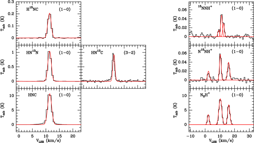
Figure 10: HNC, N₂H⁺ and their isotopologues observed spectra. Gaussian fits to the lines are superimposed to the spectra. The temperature scale is main beam temperature.

The broad emission, which is marginally visible in the HNC $(1-0)$ and HN¹³C $(2-1)$ spectra only, has not been included in our analysis (see Table 3 and Fig. 10). The HNC hyperfine structure is too narrow to be spectrally resolved in our data. However, a Population Diagram analysis applied to the $(J=1-0)$ and $(2-1)$ lines of HN¹³C, assuming extended emission, indicates moderate opacities ($\sim$0.2) and leads to an excitation temperature of 7$-$8 K. Such a low excitation temperature appears coherent with the assumption of extended emission.

As the HNC line is certainly more severely affected by opacity effect, a direct derivation of the ¹⁴N/¹⁵N ratio is not possible. From the flux ratio of ¹³C- and ¹⁵N- bearing species, the double isotopic ratio ¹³C¹⁴N/¹²C¹⁵N equal to $5.4\pm 0.8$, becomes $6.0\pm 0.8$ when the opacity correction is applied to the HN¹³C line flux.

Table 3: Integrated intensities from Gaussian fits for HNC, N₂H⁺ and their isotopologues.

HNC				HN13CN		H15NC
Transition	Eup	Frequency	$\int$Tmbdv	Frequency	$\int$Tmbdv	Frequency	$\int$Tmbdv
$(J^{\prime}-J)$	[K]	[MHz]	[K.km.s-1]	[MHz]	[K.km.s-1]	[MHz]	[K.km.s-1]
$1-0$	4.4	90663.6	21(2)	87090.9	1.7(0.2)	88865.7	0.31(0.01)
$3-2$	25.1		-	261263.3	1.09(0.04)		-
N2H+				15NNH+		N15NH+
Transition	Eup	Frequency	$\int$Tmbdv	Frequency(1)	$\int$Tmbdv	Frequency(1)	$\int$Tmbdv
$(J^{\prime}_{F^{\prime}}-J_{F})$	[K]	[MHz]	[K.km.s-1]	[MHz]	[K.km.s-1]	[MHz]	[K.km.s-1]
$1_{1}-0_{1}$	4.5	93171.9	13.1(1.5)	90263.5	0.08(0.01)	91204.3	0.059(0.008)
$1_{2}-0_{1}$	4.5	93173.7	21.3(2.5)	90263.9	0.036(0.005)	91206.0	0.09(0.02)
$1_{0}-0_{1}$	4.5	93176.1	5.3(0.5)	90264.5	0.015(0.004)	91208.5	0.025(0.006)

• The integrated intensities correspond to the narrow Gaussian components only and the 1 $\sigma$ error bars include the fit and the calibration uncertainties.

• (1) Frequencies from  Dore et al. (2009).

3.4 N₂H⁺

The main isotope and each of the ¹⁵N-bearing substitutes of N₂H⁺ show three hyperfine components, with relative intensities of 1:3:5 if LTE optically thin emission applies (see Table LABEL:tab:check). The frequencies of the hyperfine lines of ¹⁵NNH⁺ and N¹⁵NH⁺ have been presented by Dore et al. (2009). The observed hyperfine flux ratios are 1:(2.5$\pm$0.4):(4.1$\pm$0.6) for the main isotopologue, 1:(2.4$\pm$0.7):(5.0$\pm$1.5) for ¹⁵NNH⁺ and 1:(2.4$\pm$0.6):(3.8$\pm$1.2) for N¹⁵NH⁺. We conclude that, as expected, the emission of the ¹⁵N-bearing species is optically thin and that the lines opacity is very moderate for the main isotopologue components. Assuming that the weakest line of N₂H⁺ $(1-0)$ is optically thin, we can estimate the “opacity corrected fluxes” of the two others. With such a correction, the ¹⁴N/¹⁵N ratios derived from the total fluxes are $320\pm 60$ from ¹⁵NNH⁺ and $240\pm 50$ from N¹⁵NH⁺.

3.5 CN

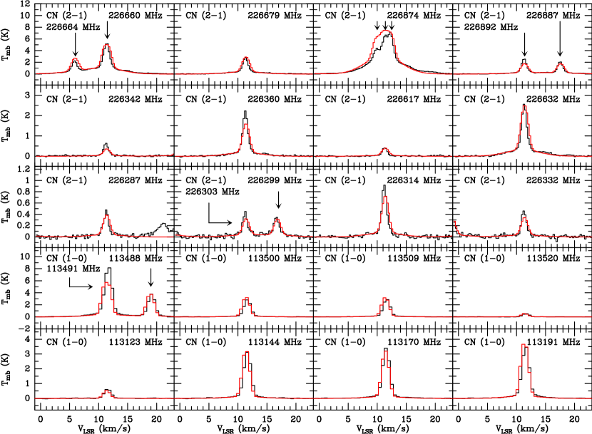
Figure 11: CN observed spectra. The profiles superimposed to the spectra have been calculated with a two components LTE modeling (see text). When several close hyperfine components are present, the frequency of the main one is given. The temperature scale is main beam temperature.

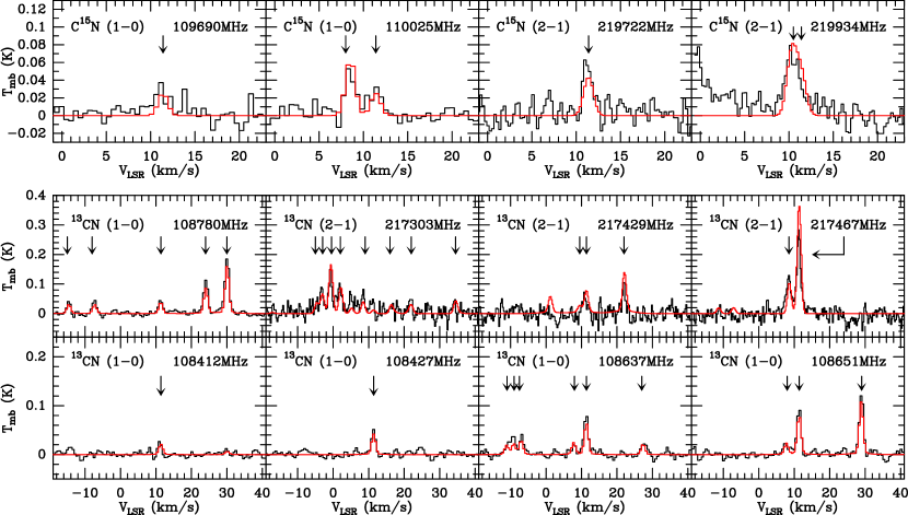
Figure 12: ¹³CN and C¹⁵Nobserved spectra. The profiles superimposed to the spectra have been calculated with a LTE modeling (see text). When several close hyperfine components are present, the frequency of the main one is given. The temperature scale is main beam temperature.

The CN family members present extremely rich rotational spectra, combining fine and hyperfine structure interactions and our survey covers both the $(N=1-0)$ and $(N=2-1)$ transitions for the three isotopologues (see Figs. 11 and 12).

In addition, the main isotopologue shows a broad emission, more visible on the $(N=2-1)$ transitions than on the $(N=1-0)$ ones.

Most of the CN $(N=1-0)$ and $(N=2-1)$ hyperfine components reported in the CDMS and JPL databases are easily detected. We have compared the observed flux ratios with the theoretical ratios (proportional to the g_up . A_ij ratios, the slight frequency differences being neglected). The results (see Table LABEL:tab:check) suggest that the hyperfine components follow an intensity distribution very close to LTE and that the line opacities are moderate.

The same analysis shows that the ¹³CN and C¹⁵N $(N=1-0)$ and $(N=2-1)$ which are clearly detected and do not suffer from blending follow an intensity distribution very close to LTE and that the lines are optically thin.

We have thus performed a simultaneous LTE modeling of the $(N=1-0)$ and $(N=2-1)$ transitions for the three isotopologues. For ¹³CN and C¹⁵N we have assumed that the emission comes from a single extended component whose kinematical properties are derived from the gaussian fits (V_LSR = 11.4 km.s^-1, FWHM = 1.3 km.s^-1). For CN, to account for the broad emission, we have added a second component (V_LSR = 11.1 km.s^-1, FWHM = 6.9 km.s^-1). The free parameters of our modelling, performed with a Markov Chain Monte-Carlo (MCMC) minimization to obtain the best fit to the lines, were the excitation temperature $T_{ex}$ and the column densities of the three isotopologues for the narrow emission component, the source size, the CN column density and the excitation temperature for the broad CN emission component.

For the first component, the best fit was obtained with the following parameters: $T_{ex}$ = $8\pm 1$ K, $N$(CN) = (3.5$\pm$0.5)$\times$10¹⁴ cm^-2, $N$(¹³CN) = (8$\pm$1)$\times$10¹² cm^-2, $N$(C¹⁵N) = (1.3$\pm$0.2)$\times$10¹² cm^-2. It corresponds to the following isotopic ratios: ¹³C¹⁴N/¹²C¹⁵N = $6.2\pm 1.3$, ¹²C/¹³C = $44\pm 8$ and ¹⁴N/¹⁵N = $270\pm 60$.

For the broad component, there are three free parameters and the best fit solution is degenerate. However, the excitation temperature depends only weakly on the assumed size and is between 50 and 60 K.

The calculated profiles are superimposed to the observed ones in Figs. 11 and Fig. 12.

Table 4: Integrated intensities from Gaussian fits for CN and its isotopologues

Species	Transition(1)	Frequency	Eup	VLSR	FWHM	$\int$Tmbdv
	$N_{J^{\prime}F^{\prime}1F^{\prime}}-N_{JF1F}$ or $N^{\prime}_{J^{\prime}F^{\prime}}-N_{JF}$	[MHz]	[K]	[km.s-1]	[km.s-1]	[K.km.s-1]
CN	1${}_{0~{}1/2~{}1/2}$ $-$ 0${}_{0~{}1/2~{}1/2}$	113123.37	5.43	11.6(0.3)	1.4(0.3)	0.9(0.1)
	1${}_{0~{}1/2~{}1/2}$ $-$ 0${}_{0~{}1/2~{}3/2}$	113144.19	5.43	11.7(0.3)	1.5(0.3)	4.9(0.5)
	1${}_{0~{}1/2~{}3/2}$ $-$ 0${}_{0~{}1/2~{}1/2}$	113170.54	5.43	11.7(0.3)	1.5(0.3)	5.3(0.5)
	1${}_{0~{}1/2~{}3/2}$ $-$ 0${}_{0~{}1/2~{}3/2}$	113191.33	5.43	11.7(0.3)	1.5(0.3)	5.6(0.6)
	1${}_{0~{}3/2~{}3/2}$ $-$ 0${}_{0~{}1/2~{}1/2}$	113488.14	5.45	11.7(0.3)	1.5(0.3)	6.0(0.7)
	1${}_{0~{}3/2~{}5/2}$ $-$ 0${}_{0~{}1/2~{}3/2}$	113490.99	5.45	11.7(0.3)	1.6(0.3)	14.0(1.6)
	1${}_{0~{}3/2~{}1/2}$ $-$ 0${}_{0~{}1/2~{}1/2}$	113499.64	5.45	11.6(0.3)	1.4(0.3)	4.3(0.4)
	1${}_{0~{}1/2~{}1/2}$ $-$ 0${}_{0~{}1/2~{}3/2}$	113508.93	5.45	11.7(0.3)	1.4(0.3)	4.5(0.5)
	1${}_{0~{}3/2~{}1/2}$ $-$ 0${}_{0~{}1/2~{}3/2}$	113520.42	5.45	11.6(0.3)	1.3(0.3)	0.8(0.1)
	2${}_{0~{}3/2~{}1/2}$ $-$ 1${}_{0~{}3/2~{}1/2}$	226287.43	16.31	11.3(0.1)	1.1(0.1)	0.5(0.1)
	2${}_{0~{}3/2~{}1/2}$ $-$ 1${}_{0~{}3/2~{}3/2}$	226298.92	16.31	11.0(0.2)	1.6(0.2)	0.6(0.2)
	2${}_{0~{}3/2~{}3/2}$ $-$ 1${}_{0~{}3/2~{}1/2}$	226303.08	16.31	11.3(0.1)	1.2(0.1)	0.5(0.1)
	2${}_{0~{}3/2~{}3/2}$ $-$ 1${}_{0~{}3/2~{}3/2}$	226314.54	16.31	11.2(0.1)	1.1(0.1)	1.0(0.2)
	2${}_{0~{}3/2~{}3/2}$ $-$ 1${}_{0~{}1/2~{}5/2}$	226332.54	16.31	11.3(0.1)	1.1(0.1)	0.5(0.1)
	2${}_{0~{}3/2~{}5/2}$ $-$ 1${}_{0~{}3/2~{}3/2}$	226341.93	16.31	11.3(0.1)	1.1(0.1)	0.7(0.1)
	2${}_{0~{}3/2~{}5/2}$ $-$ 1${}_{0~{}3/2~{}5/2}$	226359.87	16.31	11.3(0.1)	1.2(0.1)	2.6(0.6)
	2${}_{0~{}3/2~{}1/2}$ $-$ 1${}_{0~{}1/2~{}3/2}$	226616.56	16.31	11.3(0.1)	1.1(0.1)	0.5(0.1)
	2${}_{0~{}3/2~{}3/2}$ $-$ 1${}_{0~{}1/2~{}3/2}$	226632.19	16.31	11.3(0.1)	1.3(0.1)	3.2(0.7)
	2${}_{0~{}3/2~{}5/2}$ $-$ 1${}_{0~{}1/2~{}3/2}$	226659.58	16.31	11.4(0.1)	1.6(0.1)	8.3(1.7)
	2${}_{0~{}3/2~{}1/2}$ $-$ 1${}_{0~{}1/2~{}1/2}$	226663.70	16.31	11.4(0.1)	1.4(0.1)	3.2(0.7)
	2${}_{0~{}3/2~{}3/2}$ $-$ 1${}_{0~{}1/2~{}1/2}$	226679.38	16.31	11.4(0.1)	1.3(0.1)	3.6(0.8)
	2${}_{0~{}5/2~{}5/2}$ $-$ 1${}_{0~{}3/2~{}5/2}$	226892.12	16.34	11.3(0.1)	1.2(0.1)	3.2(0.7)
	2${}_{0~{}5/2~{}3/2}$ $-$ 1${}_{0~{}3/2~{}5/2}$	226905.38	16.34	11.3(0.2)	0.9(0.2)	0.10(0.03)
13CN	1${}_{1/2~{}0~{}1}$ $-$ 0${}_{1/2~{}1~{}1}$	108412.86	5.23	11.0(0.4)	1.1(0.4)	0.03(0.01)
	1${}_{1/2~{}0~{}1}$ $-$ 0${}_{1/2~{}1~{}2}$	108426.89	5.23	11.4(0.3)	1.3(0.3)	0.07(0.01)
	1${}_{3/2~{}1~{}0}$ $-$ 0${}_{1/2~{}0~{}1}$	108631.12	5.21	11.7(0.4)	1.3(0.4)	0.04(0.02)
	1${}_{3/2~{}1~{}1}$ $-$ 0${}_{1/2~{}0~{}1}$	108636.92	5.21	11.3(0.3)	1.4(0.3)	0.11(0.02)
	1${}_{3/2~{}1~{}2}$ $-$ 0${}_{1/2~{}0~{}1}$	108651.30	5.21	11.5(0.3)	1.4(0.3)	0.18(0.03)
	1${}_{1/2~{}1~{}2}$ $-$ 0${}_{1/2~{}1~{}2}$	108657.65	5.24	11.4(0.3)	1.3(0.3)	0.13(0.02)
	1${}_{3/2~{}2~{}3}$ $-$ 0${}_{1/2~{}1~{}2}$	108780.20	5.25	11.4(0.3)	1.5(0.3)	0.27(0.05)
	1${}_{3/2~{}2~{}2}$ $-$ 0${}_{1/2~{}1~{}1}$	108782.37	5.25	11.4(0.3)	1.5(0.3)	0.16(0.03)
	1${}_{3/2~{}2~{}1}$ $-$ 0${}_{1/2~{}1~{}0}$	108786.98	5.25	11.3(0.3)	1.5(0.3)	0.06(0.01)
	1${}_{3/2~{}2~{}1}$ $-$ 0${}_{1/2~{}1~{}1}$	108793.75	5.25	11.3(0.3)	1.4(0.3)	0.06(0.01)
	1${}_{3/2~{}2~{}2}$ $-$ 0${}_{1/2~{}1~{}2}$	108796.40	5.25	11.4(0.4)	1.1(0.4)	0.05(0.02)
	2${}_{5/2~{}3~{}3}$ $-$ 1${}_{3/2~{}2~{}2}$	217467.15	15.69	11.3(0.1)	1.3(0.1)	0.36(0.08)
	2${}_{5/2~{}3~{}2}$ $-$ 1${}_{3/2~{}2~{}1}$	217469.15	15.69	11.2(0.1)	1.8(0.1)	0.23(0.05)
C15N	1${}_{1/2~{}1}$ $-$ 0${}_{1/2~{}1}$	109689.61	5.27	11.1(0.4)	2.1(0.4)	0.05(0.02)
	1${}_{3/2~{}1}$ $-$ 0${}_{1/2~{}0}$	110023.54	5.28	11.5(0.3)	1.3(0.3)	0.05(0.02)
	1${}_{3/2~{}2}$ $-$ 0${}_{1/2~{}1}$	110024.59	5.28	11.4(0.4)	1.3(0.4)	0.08(0.02)
	2${}_{3/2~{}2}$ $-$ 1${}_{1/2~{}1}$	219722.49	15.81	11.3(0.2)	1.3(0.2)	0.08(0.02)
	2${}_{5/2~{}2}$ $-$ 1${}_{3/2~{}1}$	219934.04	15.84	11.4(0.1)	1.7(0.1)	0.10(0.03)

• (1) For CN and ¹³CN, according to the CDMS convention, the quantum numbers are N, J, F₁, F with F₁ = J + I₁, F = F₁ + I₂ where I₁ is the ¹²C or ¹³C nuclear spin and I₂ that of ¹⁴N. For C¹⁵N, the quantum numbers are N, J, F with J = N + S and F = J + I, where S and I are respectively the electronic spin and the nuclear spin of ¹⁵N.

• (2) The kinematical parameters and the integrated intensities correspond to the narrow Gaussian components only and the 1 $\sigma$ error bars include the fit and the calibration uncertainties.

4 Discussion and conclusions

4.1 The ¹⁴N/¹⁵N ratio towards OMC-2 FIR4

We have reported here a complete census of the ¹⁴N/¹⁵N ratio in the most abundant N-bearing species towards the protocluster OMC-2 FIR4. The five ¹⁴N/¹⁵N ratios derived directly from the line fluxes (HC₃N, CN, N₂H⁺, H¹³CN) appear very similar. Their weighted average is $260\pm 30$. Two indirect ¹⁴N/¹⁵N ratio derivations, obtained with HCN and HNC, can be made from the double isotopic ratios ¹³C¹⁴N / ¹²C¹⁵N. Discussing the ¹²C/¹³C isotopic ratio is outside of the scope of this study. However, it can just be noticed that one of the ¹³C-bearing isotopologues of HC₃N seems to show systematically stronger lines than the two others (see Fig. 2) but this requires complementary observations to be confirmed and discussed. Although far from complete in terms of ¹²C/¹³C measurements, our data allow to derive five direct estimates of this isotopic ratio and its weighted average value is $50\pm 5$. The resulting indirect ¹⁴N/¹⁵N ratios are respectively $270\pm 50$ and $290\pm 50$ for HCN and HNC. These values are in remarkable agreement with the direct determinations. The total weighted average including both direct and indirect measures is $270\pm 30$. All the ¹⁴N/¹⁵N ratios derived in OMC-2 FIR4 are plotted in Fig. 3.

As discussed for each species, the narrow emission of HCN, HNC and CN, from which the ¹⁴N/¹⁵N ratio is measured, shows a very low excitation temperature ($6-9$ K). Without large scale emission maps for these species, we cannot firmly establish that they trace extended parent gas of the protocluster but it seems a reasonable interpretation. HC₃N narrow emission traces at least 2 components: a relatively cold gas (T_ex = 25K), that our recent observations obtained with the 30m telescope show to be extended, and a warmer component (T_ex $\sim$ 50 K). A more sophisticated analysis of the HC₃N emission, included also the broad emission will be presented in a forthcoming article (Jaber Al-Edhari et al., in prep.). In addition, we also tentatively measured with the HCN isotopologues the ¹⁴N/¹⁵N ratio in the broad emission, detected for the main isotopologue of all the species studied here, except N₂H⁺. This ratio appears perfectly compatible with the value derived from the narrow emission. Our data suggest that this broad emission is warmer than the narrow one but do not allow to estimate the emission size. We hope that the interferometric (ALMA and NOEMA) data that we will soon obtain towards this source will allow to understand the nature of this emission.

4.2 Comparison with other galactic sources

Measurements of the the ¹⁴N/¹⁵N ratio in starless cores (e.g. Hily-Blant et al. (2013)) and in protostars (e.g. Wampfler et al. (2014)) seem to indicate (see Fig. 3) that the ratios derived from molecules carrying the amine functional group (NH₃, N₂H⁺) are larger than the ratios derived from molecules carrying the nitrile functional group (CN, HCN), a chemical origin being proposed for this effect. However, none of the studied sources shows a complete set of measurements from different tracers so that it is very difficult to distinguish between variations from source to source and from molecule to molecule. On the other hand, our results, which rely on a set of five different species that trace the same (cold extended) gas, and that belong to the nitrile and amine families, do not show any significant difference. In contrast, they are very similar, and they remarkably agree with the present local ¹⁴N/¹⁵N galactic ratio of $\sim 300$ as derived from observations ( Adande & Ziurys (2012);  Hily-Blant et al. (2017) and references therein) and predicted by models of galactic CNO evolution (e.g.  Romano et al. (2017)).

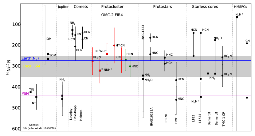
Figure 3: Nitrogen isotopic composition of Solar System objects compared with different sources (figure adapted from Hily-Blant et al. (2013)). The blue horizontal line represents the nitrogen isotopic composition of the terrestrial atmosphere(¹⁴N/¹⁵N=272), while the magenta horizontal line indicates the protosolar nebula (PSN) value of $441\pm 6$ Marty (2012). Square and circle symbols correspond to amine and nitrile functional groups, respectively. IOM means Insoluble Organic Matter, SOM Soluble Organic Matter, and CAI Calcium-, Aluminum-rich Inclusions. Red and green symbols represent respectively direct and indirect measurements of ¹⁴N/¹⁵N in OMC-2 FIR4, assuming ¹²C/¹³C =$50\pm 5$ (this work). Protostars data are from  Wampfler et al. (2014), starless cores data from Hily-Blant et al. (2013) and Taniguchi & Saito (2017), and high mass star forming cores data from  Fontani et al. (2015) (where HMSC: high-mass starless core). The local galactic ratio range, shown as a grey zone, takes into account the measurements reported in  Adande & Ziurys (2012) and  Hily-Blant et al. (2017)

Our observations show that in OMC-2 FIR4, which is the best analogue of the Sun progenitor, there is no ¹⁵N fractionation, compared to the nowadays value at the same (8 kpc) galactic center distance. This is in agreement with the recent model predictions by Roueff et al. (2015).

In conclusion, the presented measurements of ¹⁴N/¹⁵N seem to be at odd with the previous measurements in pre-stellar cores and protostars (see Fig. 3 ), which, depending on the used species, suggest ¹⁵N enrichment or deficiency with respect to the local ISM value. It is possible that this discrepancy is due to the different spatial scale probed by our and the others’ observations. Specifically, while the cold and large scale gas might not be ¹⁵N enriched, local smaller scale clumps might present this enrichment (or deficiency). On going interferometric observations towards OMC-2 FIR4 will verify this possibility. If this is the case, the enrichment of the Solar System bodies could find an explanation in the ISM chemistry. If, on the contrary, the new observations would confirm the absence of ¹⁵N enrichment also at small scales, then the ¹⁵N enrichment in Solar System bodies must have another nature.

Appendix A Observed Lines

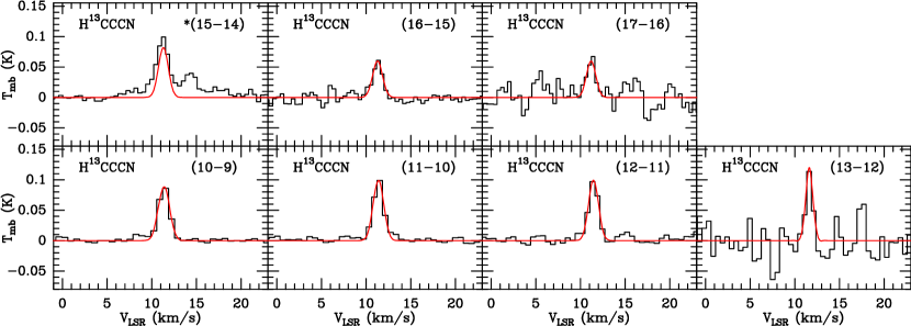
Figure 5: H¹³CCCN observed spectra and Gaussian fit to the lines. The temperature scale is main beam temperature. Due to significant overlaping with other emissions the line indicated by an asterisc (*) has not been included in our analysis nor reported in Table 1.

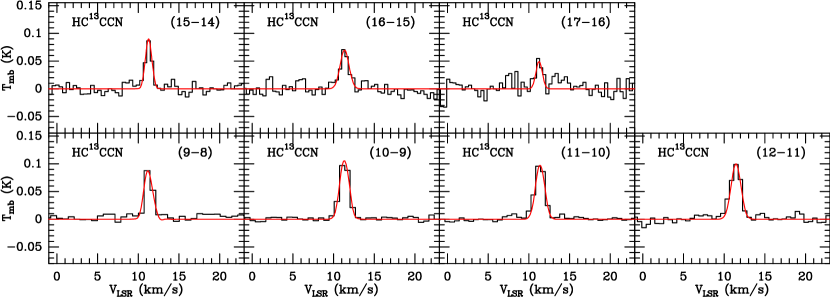
Figure 6: HC¹³CCN observed spectra and Gaussian fit to the lines. The temperature scale is main beam temperature.

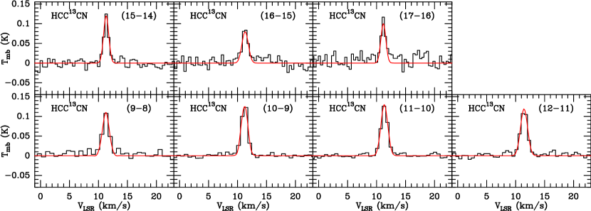
Figure 7: HCC¹³CN observed spectra and Gaussian fit to the lines. The temperature scale is main beam temperature.

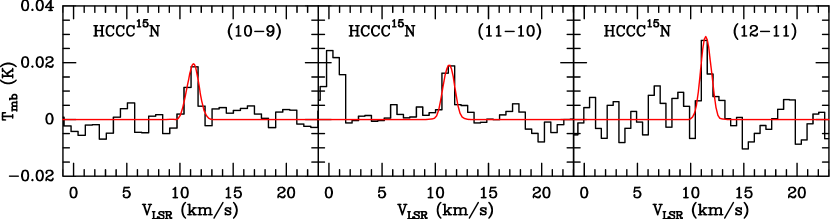
Figure 8: HCCC¹⁵N observed spectra and Gaussian fit to the lines. The temperature scale is main beam temperature.

Appendix B Opacity checks of hyperfine components

Table 5: Relative fluxes of the hyperfine components.

Species	Transition	Frequency	Eup	gup	Aij	R_theo.(1)	$\int$Tmbdv(2)	R_obs.(3)
		[MHz]	[K]		[s-1]		[K.km.s-1]
HCN	11 $-$ 01	88630.42	4.25	3	2.43$\times 10^{-5}$	3.0	8.4(0.9)	1.6(0.2)
	12 $-$ 01	88631.85	4.25	5	2.43$\times 10^{-5}$	5.0	13.5(2.0)	2.6(0.5)
	10 $-$ 01*	88633.94	4.25	1	2.43$\times 10^{-5}$	1.0	5.2(0.5)	1.0(0.1)
H13CN	11 $-$ 01	86338.77	4.14	3	2.22$\times 10^{-5}$	3.0	1.3(0.1)	2.9(0.5)
	12 $-$ 01	86340.18	4.14	5	2.22$\times 10^{-5}$	5.0	2.2(0.2)	5.1(0.9)
	10 $-$ 01*	86342.27	4.14	1	2.22$\times 10^{-5}$	1.0	0.44(0.06)	1.0(0.2)
NNH+	11 $-$ 01	93171.88	4.47	9	3.63$\times 10^{-5}$	3.0	13.1(1.5)	2.5(0.4)
	12 $-$ 01	93173.70	4.47	15	3.63$\times 10^{-5}$	5.0	21.3(2.5)	4.1(0.6)
	10 $-$ 01*	93176.13	4.47	3	3.63$\times 10^{-5}$	1.0	5.3(0.5)	1.0(0.1)
15NNH+	12 $-$ 01	90263.91	4.38	3	3.30$\times 10^{-5}$	3.0	0.036(0.005)	2.4(0.7)
	11 $-$ 01	90263.49	4.38	5	3.30$\times 10^{-5}$	5.0	0.08(0.01)	5.0(1.5)
	10 $-$ 01*	90264.50	4.38	1	3.30$\times 10^{-5}$	1.0	0.015(0.004)	1.0(0.4)
N15NH+	11 $-$ 01	91204.26	4.33	3	3.40$\times 10^{-5}$	3.0	0.059(0.008)	2.4(0.6)
	12 $-$ 01	91205.99	4.33	5	3.40$\times 10^{-5}$	5.0	0.09(0.02)	3.8(1.2)
	10 $-$ 01*	91208.52	4.33	1	3.40$\times 10^{-5}$	1.0	0.025(0.006)	1.0(0.3)
CN	1${}_{0~{}1/2~{}1/2}$ $-$ 0${}_{0~{}1/2~{}1/2}$*	113123.37	5.43	2	1.29$\times 10^{-6}$	1.0	0.9(0.1)	1.1(0.2)
	1${}_{0~{}1/2~{}1/2}$ $-$ 0${}_{0~{}1/2~{}3/2}$	113144.19	5.43	2	1.05$\times 10^{-5}$	8.1	4.9(0.5)	5.8(0.8)
	1${}_{0~{}1/2~{}3/2}$ $-$ 0${}_{0~{}1/2~{}1/2}$	113170.54	5.43	4	5.14$\times 10^{-6}$	7.9	5.3(0.5)	6.2(0.9)
	1${}_{0~{}1/2~{}3/2}$ $-$ 0${}_{0~{}1/2~{}3/2}$	113191.33	5.43	4	6.68$\times 10^{-6}$	10.3	5.6(0.6)	6.6(1.0)
	1${}_{0~{}3/2~{}3/2}$ $-$ 0${}_{0~{}1/2~{}1/2}$	113488.14	5.45	4	6.73$\times 10^{-6}$	10.4	6.0(0.7)	7.0(1.1)
	1${}_{0~{}3/2~{}5/2}$ $-$ 0${}_{0~{}1/2~{}3/2}$	113490.99	5.45	6	1.19$\times 10^{-5}$	27.5	14.0(1.6)	16.4(2.5)
	1${}_{0~{}3/2~{}1/2}$ $-$ 0${}_{0~{}1/2~{}1/2}$	113499.64	5.45	2	1.06$\times 10^{-5}$	8.2	4.3(0.4)	5.1(0.7)
	1${}_{0~{}3/2~{}3/2}$ $-$ 0${}_{0~{}1/2~{}3/2}$	113508.93	5.45	4	5.19$\times 10^{-6}$	8.0	4.5(0.5)	5.3(0.8)
	1${}_{0~{}3/2~{}1/2}$ $-$ 0${}_{0~{}1/2~{}3/2}$*	113520.42	5.45	2	1.30$\times 10^{-6}$	1.0	0.76(0.08)	0.9(0.1)
	2${}_{0~{}3/2~{}1/2}$ $-$ 1${}_{0~{}3/2~{}1/2}$	226287.43	16.31	2	1.03$\times 10^{-5}$	4.6	0.5(0.1)	5.1(1.1)
	2${}_{0~{}3/2~{}1/2}$ $-$ 1${}_{0~{}3/2~{}3/2}$	226298.92	16.31	2	8.23$\times 10^{-6}$	3.7	0.6(0.2)	5.8(1.7)
	2${}_{0~{}3/2~{}3/2}$ $-$ 1${}_{0~{}3/2~{}1/2}$	226303.08	16.31	4	4.17$\times 10^{-6}$	3.7	0.5(0.1)	4.9(1.2)
	2${}_{0~{}3/2~{}3/2}$ $-$ 1${}_{0~{}3/2~{}3/2}$	226314.54	16.31	4	9.91$\times 10^{-6}$	8.8	1.0(0.2)	10.1(2.1)
	2${}_{0~{}3/2~{}3/2}$ $-$ 1${}_{0~{}1/2~{}5/2}$	226332.54	16.31	4	4.55$\times 10^{-6}$	4.0	0.5(0.1)	5.0 (1.1)
	2${}_{0~{}3/2~{}5/2}$ $-$ 1${}_{0~{}3/2~{}3/2}$	226341.93	16.31	6	3.16$\times 10^{-6}$	4.2	0.7(0.1)	6.6(1.4)
	2${}_{0~{}3/2~{}5/2}$ $-$ 1${}_{0~{}3/2~{}5/2}$	226359.87	16.31	6	1.61$\times 10^{-5}$	21.4	2.6(0.6)	25.4(5.3)
	2${}_{0~{}3/2~{}1/2}$ $-$ 1${}_{0~{}1/2~{}3/2}$	226616.56	16.31	2	1.07$\times 10^{-5}$	4.8	0.5(0.1)	4.6(0.9)
	2${}_{0~{}3/2~{}3/2}$ $-$ 1${}_{0~{}1/2~{}3/2}$	226632.19	16.31	4	4.26$\times 10^{-5}$	37.9	3.2(0.7)	31.2(6.8)
	2${}_{0~{}3/2~{}5/2}$ $-$ 1${}_{0~{}1/2~{}3/2}$	226659.58	16.31	6	9.47$\times 10^{-5}$	126.2	8.3(1.7)	80(17)
	2${}_{0~{}3/2~{}1/2}$ $-$ 1${}_{0~{}1/2~{}1/2}$	226663.70	16.31	2	8.46$\times 10^{-5}$	37.6	3.2(0.7)	30.9(6.6)
	2${}_{0~{}3/2~{}3/2}$ $-$ 1${}_{0~{}1/2~{}1/2}$	226679.38	16.31	4	5.27$\times 10^{-5}$	46.8	3.6(0.8)	35.0 (7.3)
	2${}_{0~{}5/2~{}5/2}$ $-$ 1${}_{0~{}3/2~{}5/2}$	226892.12	16.34	6	1.81$\times 10^{-5}$	24.1	3.2(0.7)	30.9 (6.5)
	2${}_{0~{}5/2~{}3/2}$ $-$ 1${}_{0~{}3/2~{}5/2}$*	226905.38	16.34	4	1.13$\times 10^{-6}$	1.0	0.10(0.03)	1.0(0.3)
13CN	1${}_{1/2~{}0~{}1}$ $-$ 0${}_{1/2~{}1~{}1}$	108412.86	5.23	3	3.1$\times 10^{-6}$	1.1	0.03(0.01)	1.1(0.5)
	1${}_{1/2~{}0~{}1}$ $-$ 0${}_{1/2~{}1~{}2}$	108426.89	5.23	3	6.3$\times 10^{-6}$	2.3	0.069(0.008)	2.1(0.7)
	1${}_{1/2~{}1~{}0}$ $-$ 0${}_{1/2~{}0~{}1}$	108631.12	5.21	1	9.6$\times 10^{-6}$	1.2	0.04(0.02)	1.1(0.7)
	1${}_{1/2~{}1~{}1}$ $-$ 0${}_{1/2~{}0~{}1}$	108636.92	5.21	3	9.6$\times 10^{-6}$	3.5	0.11(0.02)	3.4(1.1)
	1${}_{1/2~{}1~{}2}$ $-$ 0${}_{1/2~{}0~{}1}$	108651.30	5.21	5	9.8$\times 10^{-6}$	5.9	0.18(0.03)	5.4(1.9)
	1${}_{3/2~{}1~{}2}$ $-$ 0${}_{1/2~{}1~{}2}$	108657.65	5.24	5	7.2$\times 10^{-6}$	4.4	0.13(0.02)	4.0(1.3)
	1${}_{3/2~{}2~{}3}$ $-$ 0${}_{1/2~{}1~{}2}$	108780.20	5.25	7	1.1$\times 10^{-5}$	8.9	0.27(0.05)	8.2(2.8)
	1${}_{3/2~{}2~{}2}$ $-$ 0${}_{1/2~{}1~{}1}$	108782.37	5.25	5	7.8$\times 10^{-6}$	4.7	0.16(0.03)	4.9(1.6)
	1${}_{3/2~{}2~{}1}$ $-$ 0${}_{1/2~{}1~{}0}$	108786.98	5.25	3	5.7$\times 10^{-6}$	2.1	0.06(0.01)	2.0(0.7)
	1${}_{3/2~{}2~{}1}$ $-$ 0${}_{1/2~{}1~{}1}$	108793.75	5.25	3	4.5$\times 10^{-6}$	1.6	0.06(0.01)	1.9(0.6)
	1${}_{3/2~{}2~{}2}$ $-$ 0${}_{1/2~{}1~{}2}$	108796.40	5.25	5	2.8$\times 10^{-6}$	1.7	0.05(0.02)	1.7(0.8)
	1${}_{3/2~{}1~{}2}$ $-$ 0${}_{1/2~{}1~{}1}$	108643.59	5.24	5	2.6$\times 10^{-6}$	1.6	0.06(0.01)	1.7(0.6)
	1${}_{3/2~{}1~{}0}$ $-$ 0${}_{1/2~{}1~{}1}$	108644.35	5.24	1	9.6$\times 10^{-6}$	1.2	0.06(0.02)	1.8(0.7)
	1${}_{3/2~{}1~{}1}$ $-$ 0${}_{1/2~{}1~{}1}$*	108645.06	5.24	3	2.7$\times 10^{-6}$	1.0	0.03(0.01)	1.0(0.4)
	1${}_{3/2~{}1~{}1}$ $-$ 0${}_{1/2~{}1~{}2}$	108658.95	5.24	3	3.3$\times 10^{-6}$	1.2	0.03(0.01)	1.0(0.5)
	2${}_{5/2~{}3~{}3}$ $-$ 1${}_{3/2~{}2~{}2}$	217467.15	15.69	7	8.92$\times 10^{-5}$	0.6	0.36(0.08)	0.6(0.1)
	2${}_{5/2~{}3~{}2}$ $-$ 1${}_{3/2~{}2~{}1}$	217469.15	15.69	5	8.43$\times 10^{-5}$	0.4	0.23(0.05)	0.4(0.1)
C15N	1${}_{1/2~{}1}$ $-$ 0${}_{1/2~{}1}$*	109689.61	5.27	3	7.10$\times 10^{-6}$	1.0	0.05(0.02)	1.0(0.5)
	1${}_{3/2~{}1}$ $-$ 0${}_{1/2~{}1}$	110023.54	5.28	3	7.16$\times 10^{-6}$	1.0	0.05(0.02)	1.0(0.4)
	1${}_{3/2~{}2}$ $-$ 0${}_{1/2~{}1}$	110024.59	5.28	5	1.09$\times 10^{-5}$	2.6	0.08(0.02)	1.7(0.7)
	2${}_{3/2~{}2}$ $-$ 1${}_{1/2~{}1}$	219722.49	15.81	5	8.67$\times 10^{-5}$	0.3	0.08(0.02)	0.4(0.1)
	2${}_{5/2~{}2}$ $-$ 1${}_{3/2~{}1}$	219934.04	15.84	5	9.36$\times 10^{-5}$	0.7	0.10(0.03)	0.6(0.1)

• Weakest detected line of the hyperfine structure. This is the reference to compute R_theo and R_obs

• Ratio of the line G_up A_ij product relative to the reference line; equal to the fluxes ratio in LTE optically thin conditions, neglecting the frequency differences.

• Observed lines fluxes derived from gaussian fits ; the errors include fit and calibration uncertainties.

• Ratio of observed fluxes relative to the reference line. For CN $(N=1-0)$, the reference flux is averaged over the 2 reference lines.

References

- (1)
- Adande & Ziurys (2012) Adande, G. R., & Ziurys, L. M. 2012, ApJ, 744, 194
- Aléon (2010) Aléon, J. 2010, ApJ, 722, 1342
- Bizzocchi et al. (2013) Bizzocchi, L., Caselli, P., Leonardo, E., & Dore, L. 2013, A&A, 555, A109
- Bonal et al. (2010) Bonal, L., Huss, G. R., Krot, A. N., et al. 2010, Geochim. Cosmochim. Acta, 74, 6590
- Busemann et al. (2006) Busemann, H., Alexander, C. M. O., Nittler, L. R., et al. 2006, Meteoritics and Planetary Science Supplement, 41, 5327
- Caselli & Ceccarelli (2012) Caselli, P., & Ceccarelli, C. 2012, A&A Rev., 20, 56
- Ceccarelli et al. (2014a) Ceccarelli, C., Caselli, P., Bockelée-Morvan, D., et al. 2014a, Protostars and Planets VI, 859
- Ceccarelli et al. (2014b) Ceccarelli, C., Dominik, C., López-Sepulcre, A., et al. 2014b, ApJ, 790, L1
- Cleeves et al. (2015) Cleeves, L. I., Bergin, E. A., Qi, C., Adams, F. C., & Öberg, K. I. 2015, ApJ, 799, 204
- Daniel et al. (2013) Daniel, F., Gérin, M., Roueff, E., et al. 2013, A&A, 560, A3
- Dore et al. (2009) Dore, L., Bizzocchi, L., Degli Esposti, C., & Tinti, F. 2009, A&A, 496, 275
- Fontani et al. (2015) Fontani, F., Caselli, P., Palau, A., Bizzocchi, L., & Ceccarelli, C. 2015, ApJ, 808, L46
- Fontani et al. (2017) Fontani, F. Ceccarelli, C., Favre, C., Caselli, P., Neri, R., Sims, I. R., Kahane, C., Alves, F. O., Balucani, N., Bianchi, E., et al. 2017, A&A, 605, 57
- Furlan et al. (2014) Furlan, E., Megeath, S. T., Osorio, M., et al. 2014, ApJ, 786, 26
- Gerin et al. (2009) Gerin, M., Marcelino, N., Biver, N., et al. 2009, A&A, 498, L9
- Guzmán et al. (2015) Guzmán, V. V., Öberg, K. I., Loomis, R., & Qi, C. 2015, ApJ, 814, 53
- Guzmán et al. (2017) Guzmán, V. V., Öberg, K. I., Huang, J., Loomis, R., & Qi, C. 2017, ApJ, 836, 30
- Hily-Blant et al. (2013) Hily-Blant, P., Bonal, L. Faure, A. & Quirico, E. 2013, Icarus, 223, 582
- Hily-Blant et al. (2017) Hily-Blant, P., Magalhaes, V., Kastner, J., Faure, A. Forveille, T., & Qi, C. 2017, A&A, 603, L6.
- Hirota et al. (2007) Hirota, T., Bushimata, T., Choi, Y. K., et al. 2007, PASJ, 59, 897
- Ikeda et al. (2002) Ikeda, M., Hirota, T., & Yamamoto, S. 2002, ApJ, 575, 250
- López-Sepulcre et al. (2013) López-Sepulcre, A., Taquet, V., Sánchez-Monge, Á., et al. 2013, A&A, 556, A62
- Manfroid et al. (2009) Manfroid, J., Jehin, E., Hutsemékers, D., et al. 2009, A&A, 503, 613
- Marty (2012) Marty, B. 2012, Earth Planet Sci Lett 313, 56
- Menten et al. (2007) Menten, K. M., Reid, M. J., Forbrich, J., & Brunthaler, A. 2007, A&A, 474, 515
- Milam & Charnley (2012) Milam, S. N., & Charnley, S. B. 2012, in Lunar and Planetary Science Conference, Vol. 43, Lunar and Planetary Science Conference, 2618
- Mumma & Charnley (2011) Mumma, M. J., & Charnley, S. B. 2011, ARA&A, 49, 471
- Rodgers & Charnley (2008) Rodgers, S. D., & Charnley, S. B. 2008, ApJ, 689, 1448
- Romano et al. (2017) Romano, D., Matteucci, F., Zhang, Z.-Y., Papadopoulos, P. P., & Ivison, R. J. 2017, MNRAS, 470, 401
- Roueff et al. (2015) Roueff, E., Loison, J. C., & Hickson, K. M. 2015, A&A, 576, A99
- Rousselot et al. (2014) Rousselot, P., Pirali, O., Jehin, E., et al. 2014, ApJ, 780, L17
- Shimajiri et al. (2008) Shimajiri, Y., Takahashi, S., Takakuwa, S., Saito, M., & Kawabe, R. 2008, ApJ, 683, 255
- Shinnaka et al. (2014) Shinnaka, Y., Kawakita, H., Kobayashi, H., Nagashima, M., & Boice, D. C. 2014, ApJ, 782, L16
- Taniguchi & Saito (2017) Taniguchi, K., & Saito, M. 2017, ArXiv e-prints, arXiv:1706.08662
- Terzieva & Herbst (2000) Terzieva, R., & Herbst, E. 2000, MNRAS, 317, 563
- Vastel et al. (2015) Vastel, C., Bottinelli, S., Caux, E., Glorian, J.-M., & Boiziot, M. 2015, Proceedings of the Annual meeting of the French Society of Astronomy and Astrophysics. Eds.: F. Martins, S. Boissier, V. Buat, L. Cambrésy, P. Petit, pp.313-316
- Wampfler et al. (2014) Wampfler, S. F., Jørgensen, J. K., Bizzarro, M., & Bisschop, S. E. 2014, A&A, 572, A24
- Wirström et al. (2012) Wirström, E. S., Charnley, S. B., Cordiner, M. A., & Milam, S. N. 2012, ApJ, 757, L11