Progress of the Development of the ELI-NP GBS High Level Applications

Abstract

The Gamma Beam System (GBS) is a high brightness LINAC to be installed in Magurele (Bucharest) at the new ELI-NP (Extreme Light Infrastructure - Nuclear Physics) laboratory. The accelerated electrons, with energies ranging from 280 to 720 MeV, will collide with a high power laser to produce tunable high energy photons (0.2-20MeV ) with high intensity ($10^{13}$ photons/s), high brilliance and spectral purity ($0.1\%$BW), through the Compton backscattering process. This light source will be open to users for nuclear photonics and nuclear physics advanced experiments. Tested high level applications will play an important role in commissioning and operation. In this paper we report the progress and status of the development of dedicated high level applications. We also present the results of the test on the FERMI LINAC of the electron trajectory control method based on Dispersion Free Steering.

1 Introduction

Any particle accelerator is an ensemble of many different complex devices and systems. Each subsystem is properly integrated in a control system, which enables the operator to access the data in read/write mode. A set of procedures which act on data accessible by the control system is called “application” on the machine. A High Level Application (HLA) is a set of automated commands or operations that perform a specific measurement/characterization on the machine. We want to have the possibility to test the applications on a virtual accelerator before the GBS LINAC commissioning[1]. The control system (CS) of the ELI-GBS is based on EPICS, which is a distributed software framework based on a client-server architecture[2]. The data from devices is put on the EPICS Channel Access (CA) communication protocol, from which it is accessible by the client services in the network.

Matlab Middle Layer (MML)[3, 4, 5, 6] is the framework chosen to develop the high level applications. MML consists of a library of Matlab files that enable the development of control applications for particle accelerators control. An operator can access Process Variables (PVs) on the machine control system I/O Controllers (IOC) or on a machine model. MML software development is aimed to allow accelerator physicists to develop more easily the required high level functions for a proper operation of the machine.

The most basic MML functions are used to communicate either with the online machine or with the virtual one. The two main functions for data access are $getpv$ and $setpv$. Access to the accelerator hardware is handled through machine-specific routines to acquire and control database parameters csuch as BPMs, Magnets, RF systems. Depending on whether the program is in the simulate or on-line mode, the $getpv$ and $setpv$ commands communicate with the MATLAB Accelerator Toolbox (simulation) or with actual hardware via EPICS CA (on-line).

2 eleMML Architecture

The integration of the physics engine of $\mathsf{elegant}$[7] with the power of MATLAB enables to develop and test applications on the ELI-GBS virtual machine, through the Self Describing Data Sets (SDDS) file protocol[8]. The result is eleMML i.e. a set of software tools developed to interface MML with elegant and to use the latter as a physics engine for the “model” operation of High Level Applications. An overview of the architecture of eleMML is presented in Fig. 1.

The core of eleMML tool-set is the development of a software function called $\mathsf{sddsReadAny}$ which imports data from sdds-type files into the Matlab workspace, linking each column or parameter in the input sdds file into a column array. SDDS Toolkit provides a basic link between Matlab and elegant through the SDDSMatlab library. This contains the $\mathsf{sddsload}$ function, which imports an sdds file into a Matlab structure-type variable. The $\mathsf{sddsReadAny}$ function goes one step further in providing the user directly with the simulation output data. When a setpv call is made, the simulation data is updated and element parameters changed. In order to write data to the different elements in the simulation mode, we exploit the $\mathsf{-macro}$ option of $\mathsf{elegant}$ call. The $\mathsf{-macro}$ option allows performing text substitutions in the command stream. Multiple $\mathsf{-macro}$ options may be given. A system call is made from Matlab when setpv is invoked.

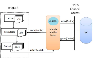
Figure 1: Schematic diagram of the architecture of eleMML

In preparation for the commissioning and operations of ELI-NP GBS, a dedicated “virtual accelerator” (VA) or “Model Server” has been created. This virtual test platform simulates the LINAC response to HLA commands. It is based on a soft IOC i.e. a database of process variable records not associated with real hardware but that can be used to simulate the behavior of a real device. The soft IOC PVs can be configured directly from simulated sdds output files, and written to the CA process variables relative to hardware devices or general machine, as schematically illustrated in Fig. 2.

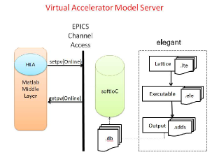
Figure 2: Virtual test platform that simulates the LINAC response to HLA commands

3 Simulated bunch length measurement

One of the first applications needed for commissioning is the bunch length measurement[9], for which a model server was set up to simulate the real measure. Bunch length measurement procedure is based onthe actual measurement. The bunch length procedure is based on streaking the beam with a transverse deflecting cavity, stepping the voltage phase around the $\psi=0\,rad$ value, to measure the centroid position downstream. A linear fit is performed to correlate the vertical beam centroid at the screen $C_{y}(\psi)$ with respect to the phase itself. The slope of the linear fit is the calibration factor $K_{cal}(\psi)$ that enables to calculate the bunch length.

The results of the elegant simulations have been pushed on the VA to test the bunch length measurement application. Fig. 3 shows the screenshots of the high level application, with the operator panel on the left and the measured data on the right.

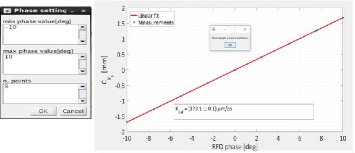
Figure 3: Screenshot of the box in which an operator can select the parameters to perform the bunch length measurement (left) and resulting measurement data (right).

4 Experimental trajectory control at Fermi

Beam trajectory control is important to maintain quality beam at the IP and subsequent properties of the radiation for the experiments. As the GBS will operate in a wide range of energies and electron beam parameter settings, LINAC properties should be optimized for all working points of the machine. The ideal operation is when the electron beam trajectory lies on the electromagnetic center of the all the active elements. There are different methods to control the trajectory and compensate misalignment, which have been studied for the low energy line of the ELI-NP GBS. As reported in [10], Dispersion Free Steering[11, 12, 13, 14] enables to optimize the beam trajectory better than other methods. We made a test of DFS at Fermi, an international FEL facility in Basovizza, Italy[15, 16]. The acceleration, compression and transport of the electron beams occupies approximately the first 300 m of the machine. The machine operates in single bunch mode. The bunch charge was 700 pC and the energy at the starting point of the correction was 1.2 GeV. We used 5 horizontal and vertical correctors on a section of the LINAC (red box in Fig. 4) comprising the last accelerating section and the transport line to the undulators’ hall. The relevant beam parameters are summarized in Table (1).

Electron beam	Value	Units
Energy	$\approx$1.3	GeV
Slice energy spread	< 0.2	MeV
Charge	700	pC
Norm. emittance	0.8-1	mm-mrad

Table 1: Summary of some of the key electron beam parameters of the working point chosen for the DFS test.

Our HLA tool were ported to the resident TANGO control system through existing Tango-MATLAB binding. Moreover, specific utilities were developed online in order to perform the measurement, and coordination with pre-existing measurement tools was achieved. In particular the Fermi LINAC has an ongoing Fast Trajectory Feedback always active. We unplugged the DFS correctors from the active feedback in order to perform our measurements and tests. The reference trajectory was the initial electron orbit set by machine operators. We used 5 horizontal and vertical correctors on a section of the LINAC comprising the last accelerating section (L04.06) and the transport line to the undulators’ hall, corresponding to the part in the rectangular box of Fig. 4. The portion is called TLS and goes from L4.06 accelerating section to the end of the transport line to the undulators.

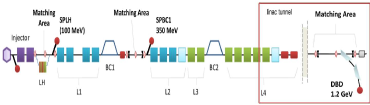
Figure 4: a) Schematic layout of the FERMI machine up to the Matching Area preceding the undulators. The red box highlights the portion of the machine on which the DFS test was performed. The diagnostic beam dump has been used to measure the energy of the test beam.

To change the beam energy, the phase of the accelerating field with respect to the electron beam in the LINAC4 accelerating section L04.06 was varied. The relative phase between the beam and the accelerating field was varied by 90°. This leads to a $\Delta E=25MeV$ between the nominal and the offset beam (about 25% relative energy difference). This is smaller than the usually introduced energy changes, which are on the order of 5% to 10%. The shot to shot orbit jitter affects the orbit measurement for the dispersion free steering. An averaging strategy can improve the measurement, as described in the following section.

4.1 Experimental results

The experimental procedure steps are summarized in Fig. 5.

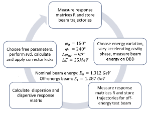
Figure 5: Conceptual scheme of the steps needed to perform DFS correction, with details on the working point of the off-energy beam chosen to perform our measurement.

Dispersion measurement is based on measuring the orbit for different beam energies which can be expressed as

$$D=\frac{\delta x}{\nicefrac{{\Delta E}}{{E}}}=\frac{x(E_{0}(1-\delta))-x(E_{0})}{\nicefrac{{\Delta E}}{{E}}}$$ (1)

In order to achieve a stable measurement, 10 BPM samples were averaged for each trajectory and dispersion measurement, as shown in Fig. (6).

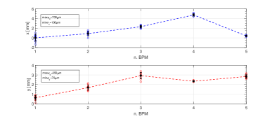
Figure 6: Before-correction: horizontal (top) and vertical (bottom) beam trajectory measurement. Empty dots: values of the position at the BPMs for ten consecutive trajectory samples acquired. The data shows the fluctuation due to launching conditions of the beam at the entrance of the LINAC. Solid line: average value with calculated $\sigma-wide$ error-bars. The text-box on the plot shows the value of the precision of the measurement . The single shot resolution of each BPM is $\sigma_{BPM}=5\mu m$.

The optimal weighting of the difference orbit with respect to the nominal orbit was determined to be $\omega=1$0. This is chosen empirically altough a theoretical estimate can be obtained from

$$\omega=\frac{\sigma_{bpm\,res}^{2}+\sigma_{bpm\,align}^{2}}{2\sigma_{bpm\,res}^{2}}$$ (2)

where $\sigma_{bpm,res}$ is the BPM precision and $\sigma_{bpm,align}$ is an estimate of the standard deviation of the BPM misalingment distribution.

Fig. (7) shows the calculated corrector kicks: the horizontal values are one order of magnitude higher than the vertical ones, as expected from the response matrix analysis.

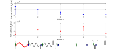
Figure 7: Horizontal(top subplot) and vertical(bottom subplot) corrector kicks calculated with DFS and applied to perform the correction.

The result of the DFS correction is summarized in Fig. (8), where the horizontal and vertical dispersion before and after correction are shown. Table 2 contains a summary of the electron beam and working point parameters for the experiment.

Parameter	Value	Unit
$E_{0}$	1.312	GeV
$E_{1}$	1.287	GeV
$\nicefrac{{\Delta E}}{{E}}$	2	%
$\omega$	10
$\beta$	1

Table 2: Summary of the free parameter values chosen for the DFS off-energy correction. $\omega$ is proportional to the ratio between residual dispersion correction and bpm-zeroing, while $\beta\neq 0$ limits the maximum corrector kick amplitudes.

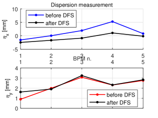
Figure 8: Measured residual dispersion before and after applying DFS correction, respectively for the horizontal (top subplot) and vertical (bottom subplot) planes.

The horizontal dispersion was corrected significantly while the vertical correction is almost negligible. An explanation for this comes from analyzing the values of the residual dispersion before the correction: in the vertical plane the initial value is lower than for the horizontal plane, thus the energy difference used for correcting the horizontal plane was insufficient for the vertical case.

DFS proved to be capable of correcting the trajectory but care had to be put into defining the free parameters $\omega,\beta$ and the energy difference $\Delta E$ between nominal and off-energy beam.

5 Summary

We have presented the status of the development of high level applications for ELI-NP GBS. Integrating elegant with MML has lead to the development of the eleMML architecture. This allows us to test the tools for commissioning on a virtual accelerator based on EPICS soft-IOCs, such as a transverse deflecting bunch length measurement application. For a complex application such as Dispersion Free Steering, we tested the method at Fermi LINAC. Fermi is a machine routinely used by international users so we didn’t expect to find very high values of residual dispersion as the machine has been already and is continuously optimized. Nevertheless the DFS method was successfully validated on an existing machine. With eleMML framework, collaborative development of more high level applications for each working group will be possible, enabling the collaboration to simulate commissioning before the machine comes online. For istance an application is under development to perform the beam-based alignment of individual accelerating sections.

—————–

References

-
[1]
A. Giribono, et al.,
ELI-NP GBS
Status, in: Proc. of International Particle Accelerator Conference
(IPAC’17), Copenhagen, Denmark, no. 8 in International Particle Accelerator
Conference, JACoW, Geneva, Switzerland, 2017, pp. 880–883,
https://doi.org/10.18429/JACoW-IPAC2017-MOPVA016.
doi:https://doi.org/10.18429/JACoW-IPAC2017-MOPVA016.
URL http://jacow.org/ipac2017/papers/mopva016.pdf -
[2]
S. Pioli, et al.,
The Turn-key
Control System for the ELI-NP Gamma Beam System, in: Proceedings, 7th
International Particle Accelerator Conference (IPAC 2016): Busan, Korea, May
8-13, 2016, 2016.
doi:10.18429/JACoW-IPAC2016-THPOY003.
URL http://inspirehep.net/record/1470719/files/thpoy003.pdf - [3] J. Corbett, G. Portmann, A. Terebilo, Accelerator control middle layer, Conf. Proc. C030512 (2003) 2369.
- [4] J. C. Gregory J. Portmann, A. Terebilo, Middle Layer Software Manual for Accelerator Control (2006).
-
[5]
G. J. Portmann, J. Corbett, A. Terebilo,
An Accelerator control middle layer
using Matlab (LBNL-PUB-925. SLAC-PUB-11445).
URL https://cds.cern.ch/record/894827 - [6] A. Terebilo, Channel access client toolbox for MATLAB, eConf C011127. arXiv:physics/0111198.
- [7] M. Borland, elegant: A flexible sdds-compliant code for accelerator simulation, Advanced Photon Source LS-287 (September 2000).
- [8] M. Borland, A self-describing file protocol for simulation integration and shared postprocessors, in: PAC’95 Proceedings, 1995.
-
[9]
L. Sabato, D. Alesini, P. Arpaia, A. Giribono, A. Liccardo, A. Mostacci,
L. Palumbo, C. Vaccarezza, A. Variola,
Metrological
Characterization of the Bunch Length Measurement by Means of a RF Deflector
at the ELI-NP Compton Gamma source, in: Proceedings, 7th International
Particle Accelerator Conference (IPAC 2016): Busan, Korea, May 8-13, 2016,
2016, p. MOPMB018.
doi:10.18429/JACoW-IPAC2016-MOPMB018.
URL http://inspirehep.net/record/1469533/files/mopmb018.pdf - [10] G. Campogiani, S. Guiducci, A. Giribono, C. Vaccarezza, A. Variola, Electron beam trajectory and optics control in the ELI-NP Gamma Beam System, Nucl. Instrum. Meth. A865 (2017) 51–54. doi:10.1016/j.nima.2016.08.055.
- [11] J. Pfingstner, E. Adli, D. Schulte, On-line dispersion estimation and correction scheme for the Compact Linear Collider, Phys. Rev. Accel. Beams 20 (1) (2017) 011006. doi:10.1103/PhysRevAccelBeams.20.011006.
-
[12]
D. Schulte, Different Options for
Dispersion Free Steering in the CLIC Main Linac.
URL https://cds.cern.ch/record/879699 - [13] T. O. Raubenheimer, R. D. Ruth, A dispersion-free trajectory correction technique for linear colliders, Nuclear Instruments and Methods in Physics Research A 302 (1991) 191–208. doi:10.1016/0168-9002(91)90403-D.
-
[14]
A. e. a. Latina, Experimental
demonstration of a global dispersion-free steering correction at the new
linac test facility at SLAC, Phys. Rev. Spec. Top. Accel. Beams 17 (4).
URL https://cds.cern.ch/record/2135837 -
[15]
E. Allaria, R. Appio, L. Badano, W. A. Barletta, S. Bassanese, S. G. Biedron,
A. Borga, E. Busetto, D. Castronovo, P. Cinquegrana, S. Cleva, D. Cocco,
M. Cornacchia, P. Craievich, I. Cudin, G. D’Auria, M. Dal Forno, M. B.
Danailov, R. De Monte, G. De Ninno, P. Delgiusto, A. Demidovich, S. Di Mitri,
B. Diviacco, A. Fabris, R. Fabris, W. Fawley, M. Ferianis, E. Ferrari,
S. Ferry, L. Froehlich, P. Furlan, G. Gaio, F. Gelmetti, L. Giannessi,
M. Giannini, R. Gobessi, R. Ivanov, E. Karantzoulis, M. Lonza, A. Lutman,
B. Mahieu, M. Milloch, S. V. Milton, M. Musardo, I. Nikolov, S. Noe,
F. Parmigiani, G. Penco, M. Petronio, L. Pivetta, M. Predonzani, F. Rossi,
L. Rumiz, A. Salom, C. Scafuri, C. Serpico, P. Sigalotti, S. Spampinati,
C. Spezzani, M. Svandrlik, C. Svetina, S. Tazzari, M. Trovo, R. Umer,
A. Vascotto, M. Veronese, R. Visintini, M. Zaccaria, D. Zangrando,
M. Zangrando, Highly
coherent and stable pulses from the fermi seeded free-electron laser in the
extreme ultraviolet 6 (10) (2012) 699–704.
URL http://dx.doi.org/10.1038/NPHOTON.2012.233 - [16] E. Allaria, D. Castronovo, P. Cinquegrana, P. Craievich, M. Dal Forno, M. B. Danailov, G. D’Auria, A. Demidovich, G. De Ninno, S. Di Mitri, B. Diviacco, W. M. Fawley, M. Ferianis, E. Ferrari, L. Froehlich, G. Gaio, D. Gauthier, L. Giannessi, R. Ivanov, B. Mahieu, N. Mahne, I. Nikolov, F. Parmigiani, G. Penco, L. Raimondi, C. Scafuri, C. Serpico, P. Sigalotti, S. Spampinati, C. Spezzani, M. Svandrlik, C. Svetina, M. Trovo, M. Veronese, D. Zangrando, M. Zangrando, Two-stage seeded soft-x-ray free-electron laser, Nature Photonics 7 (11) (2013) 913918. doi:10.1038/NPHOTON.2013.277.