A three-site gauge model for flavor hierarchies and flavor anomalies

Abstract

We present a three-site Pati-Salam gauge model able to explain the Standard Model flavor hierarchies while, at the same time, accommodating the recent experimental hints of lepton-flavor non-universality in $B$ decays. The model is consistent with low- and high-energy bounds, and predicts a rich spectrum of new states at the TeV scale that could be probed in the near future by the high-$p_{T}$ experiments at the LHC.

I Introduction

Recent data on semileptonic $B$ decays indicate anomalous violations of Lepton Flavor Universality (LFU) of short-distance origin. The statistical significance of each anomaly does not exceed the $3\sigma$ level, but the overall set of deviations from the Standard Model (SM) predictions is very consistent. The evidences collected so far can naturally be grouped into two categories, according to the underlying quark-level transition: i) deviations from $\tau/\mu$ (and $\tau/e$) universality in $b\to c\ell\bar{\nu}$ charged currents Lees:2013uzd ; Aaij:2015yra ; Hirose:2016wfn ; Aaij:2017deq ; ii) deviations from $\mu/e$ universality in $b\to s\ell\bar{\ell}$ neutral currents Aaij:2014ora ; Aaij:2017vbb . The latter turn out to be consistent Altmannshofer:2015sma ; Descotes-Genon:2015uva with the anomalies reported in the angular distributions of the $B^{0}\to K^{*0}\mu^{+}\mu^{-}$ decay Aaij:2013qta ; Aaij:2015oid .

A common origin of the two set of anomalies is not obvious, but is very appealing from the theoretical point of view. Severals attempts to provide a combined explanation of the two effects have been presented in the recent literature Bhattacharya:2014wla ; Alonso:2015sja ; Greljo:2015mma ; Calibbi:2015kma ; Bauer:2015knc ; Fajfer:2015ycq ; Barbieri:2015yvd ; Das:2016vkr ; Hiller:2016kry ; Bhattacharya:2016mcc ; Boucenna:2016wpr ; Buttazzo:2016kid ; Boucenna:2016qad ; Barbieri:2016las ; Bordone:2017anc ; Crivellin:2017zlb ; Becirevic:2016oho ; Cai:2017wry ; Megias:2017ove . Among them, a class of particularly motivated models are those based on TeV-scale new physics (NP) coupled mainly to the third generation of SM fermions, with subleading effects on the light generations controlled by an approximate $\mathrm{U(2)_{Q}}\times\mathrm{U(2)_{L}}$ flavor symmetry Barbieri:2011ci . As recently shown in Buttazzo:2017ixm (see also Greljo:2015mma ; Barbieri:2015yvd ; Bordone:2017anc ), an Effective Field Theory (EFT) based on this flavor symmetry allows us to account for the observed semileptonic LFU anomalies taking into account the tight constraints from other low-energy data Feruglio:2017rjo ; Feruglio:2016gvd . Moreover, the EFT fit singles out the case of a vector leptoquark (LQ) field $U_{\mu}\sim(\mathbf{3},\mathbf{1})_{2/3}$, originally proposed in Barbieri:2015yvd , as the simplest and most successful framework with a single TeV-scale mediator (taking into account also the direct bounds from high-energy searches Faroughy:2016osc ).

While the results of Ref. Buttazzo:2017ixm are quite encouraging, the EFT solution and the simplified models require an appropriate UV completion. In particular, the vector LQ mediator could be a composite state of a new strongly interacting sector, as proposed in Barbieri:2015yvd ; Barbieri:2016las , or a massive gauge boson of a spontaneously broken gauge theory, as proposed in Assad:2017iib ; DiLuzio:2017vat ; Calibbi:2017qbu . In this paper we follow the latter direction.

Ultraviolet completions for the vector LQ mediator $U_{\mu}$ naturally point toward variations of the Pati-Salam (PS) gauge group, PS=$\mathrm{SU(4)}\times\mathrm{SU(2)_{L}}\times\mathrm{SU(2)_{R}}$ Pati:1974yy , that contains a massive gauge field with these quantum numbers. The original PS model does not work since the (flavor-blind) LQ field has to be very heavy in order to satisfy the tight bounds from the coupling to the light generations. An interesting proposal to overcome this problem has been put forward in Ref. DiLuzio:2017vat , with an extension of the PS gauge group and the introduction of heavy vector-like fermions, such that the LQ boson couples to SM fermions only as a result of a specific mass mixing between exotic and SM fermions.

A weakness of most of the explicit SM extensions proposed so far to address the $B$-physics anomalies, including the proposal of Ref. DiLuzio:2017vat , is the fact that the flavor structure of the models is somehow ad hoc. This should be contrasted with the EFT solution of Ref. Buttazzo:2017ixm , which seems to point toward a common origin between flavor anomalies and the hierarchies of the SM Yukawa couplings. In this paper we try to address these problems together, proposing a model that is not only able to address the anomalies, but is also able to explain in a natural way the observed flavor hierarchies.

The model we propose is a three-site version of the original PS model. At high energies, the gauge group is $\mathrm{PS^{3}}\equiv\mathrm{PS_{1}}\times\mathrm{PS_{2}}\times\mathrm{PS_{3}}$, where each PS group acts on a single fermion family. The spontaneous symmetry breaking (SSB) down to the SM group occurs in a series of steps characterized by different energy scales, which allow us to decouple the heavy exotic fields coupled to the first two generations at very high energies. As a result, the gauge group controlling TeV-scale dynamics contains a LQ field that is coupled mainly to the third generation (see Fig. 1). A key aspect of this construction is the hypothesis that electroweak symmetry breaking (EWSB) occurs via a Higgs field sitting only on the third-generation site: this assumption allows us to derive the hierarchical structure of the Yukawa couplings as a consequence of the hierarchies of the vacuum expectation values (VEVs) controlling the breaking of the initial gauge group down to the SM. In particular, the $\mathrm{U(2)_{Q}}\times\mathrm{U(2)_{L}}$ global flavor symmetry appears as a subgroup of an approximate flavor symmetry of the system emerging at low energies [$\mathrm{U(2)^{5}}$]. Last but not least, the localization of the Higgs field on the third-generation site provides a natural screening mechanism for the Higgs mass term against the heavy energy scales related to the symmetry breaking of the heavy fields coupled to the light generations.

II The model

The gauge symmetry of the model holding at high energies is $\mathrm{PS}^{3}\equiv\mathrm{PS}_{1}\times\mathrm{PS}_{2}\times\mathrm{PS}_{3}$, where

$$\mathrm{PS}_{i}=\mathrm{SU(4)}_{i}\times\mathrm{[SU(2)_{L}]}_{i}\times\mathrm{[SU(2)_{R}]}_{i}~{}.$$ (1)

The fermion content is the same as in the SM plus three right-handed neutrinos, such that each fermion family is embedded in left- and right-handed multiplets of a given $\mathrm{PS}_{i}$ subgroup:

$$\Psi_{L}^{\mbox{\tiny($i$)}}\sim(\mathbf{4},\mathbf{2},\mathbf{1})_{i}\,,\qquad\Psi_{R}^{\mbox{\tiny($i$)}}\sim(\mathbf{4},\mathbf{1},\mathbf{2})_{i}\,.$$ (2)

The subindex $i=1,2,3$ denotes the site that, before any symmetry breaking, can be identified with the generation index.

The SM gauge group is a subgroup of the diagonal group, $\mathrm{PS}_{\rm diag}=\mathrm{PS}_{1+2+3}$, which corresponds to the original PS gauge group. The SSB breaking $\mathrm{PS}^{3}\to{\rm SM}$ occurs in a series of steps at different energy scales (see Fig. 1) with appropriate scalar fields acquiring non-vanishing VEVs, as described below.

I. High-scale vertical breaking [$\mathrm{PS}_{1}\to\mathrm{SM}_{1}$].
At some heavy scale, $\Lambda_{1}>10^{3}$ TeV, the $\mathrm{PS}_{1}$ group is broken to $\mathrm{SM}_{1}$, where

$$\mathrm{SM}_{i}=\mathrm{SU(3)}_{i}\times\mathrm{[SU(2)_{L}]}_{i}\times\mathrm{[U(1)_{Y}]}_{i}~{},$$ (3)

by the VEV of a scalar field $\Sigma_{1}\sim(\mathbf{4},\mathbf{1},\mathbf{2})_{1}$, charged only under $\mathrm{PS}_{1}$ (or localized on the first site). Via this breaking 9 gauge fields with exotic quantum numbers (6 LQ fields, a $W_{R}^{\pm}$, and a $Z^{\prime}$, all coupled only to the first generation) acquire a heavy mass and decouple.

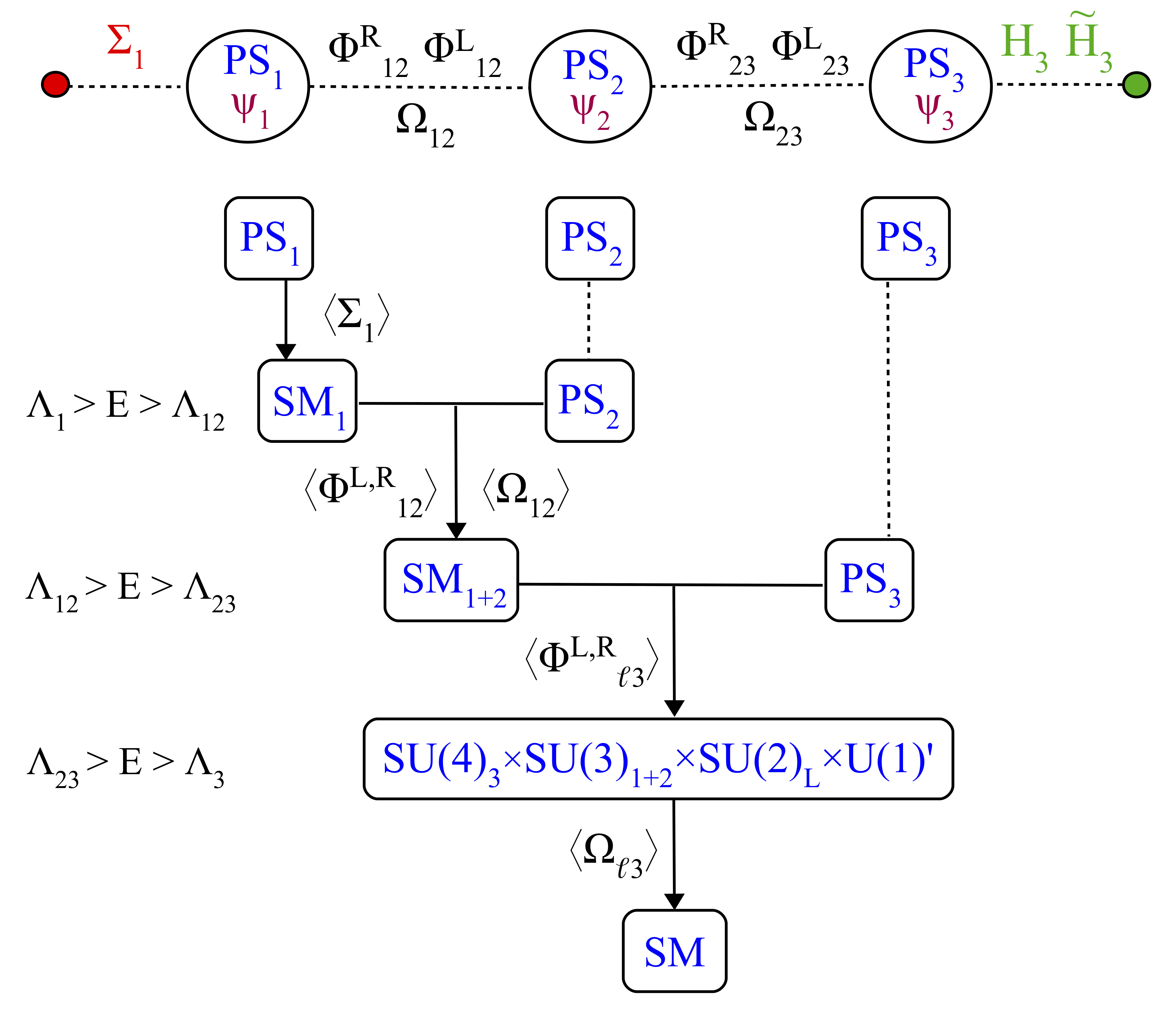
Figure 1: Moose diagram of the model (up) and symmetry breaking sequence.

II. Horizontal breaking 1–2 [$\mathrm{SM}_{1}\times\mathrm{PS}_{2}\to\mathrm{SM}_{1+2}$].
Gauge fields on different sites are broken to their diagonal subgroup via appropriate link fields, or scalar bilinears. On both links (1–2 and 2–3) we introduce the following set of link fields

$$\begin{aligned} \Phi_{ij}^{L}&\sim(\mathbf{1},\mathbf{2},\mathbf{1})_{i}\times(\mathbf{1},\mathbf{\bar{2}},\mathbf{1})_{j}~{},\\ \Phi_{ij}^{R}&\sim(\mathbf{1},\mathbf{1},\mathbf{2})_{i}\times(\mathbf{1},\mathbf{1},\mathbf{\bar{2}})_{j}~{},\\ \Omega_{ij}&\sim(\mathbf{4},\mathbf{2},\mathbf{1})_{i}\times(\mathbf{\bar{4}},\mathbf{\bar{2}},\mathbf{1})_{j}~{},\end{aligned}$$ (4)

such that

$$\begin{aligned} \langle\Phi_{ij}^{L}\rangle\not=0\,\Rightarrow&\,\mathrm{[SU(2)_{L}]}_{i}\times\mathrm{[SU(2)_{L}]}_{j}\to\mathrm{[SU(2)_{L}]}_{i+j}~{},\\ \langle\Phi_{ij}^{R}\rangle\not=0\,\Rightarrow&\,\mathrm{[SU(2)_{R}]}_{i}\times\mathrm{[SU(2)_{R}]}_{j}\to\mathrm{[SU(2)_{R}]}_{i+j}~{},\\ \langle\Omega_{ij}\rangle\not=0\,\Rightarrow&\,\left\{\begin{array}[]{l}\mathrm{SU(4)}_{i}\times\mathrm{SU(4)}_{j}\to\mathrm{SU(4)}_{i+j}\\ \mathrm{[SU(2)_{L}]}_{i}\times\mathrm{[SU(2)_{L}]}_{j}\to\mathrm{[SU(2)_{L}]}_{i+j}~{}.\end{array}\right.\end{aligned}$$

At a scale $\Lambda_{12}<\Lambda_{1}$ the 1–2 link fields acquire a VEV. As a result, the vertical breaking occurring on the first site is mediated also to the second site, and the gauge symmetry is reduced to $\mathrm{SM}_{1+2}\times\mathrm{PS}_{3}$.

Thanks to this second breaking, 9 exotic gauge fields coupled mainly to the second generation, and 12 SM-like gauge fields coupled in a non-universal way to the first two families acquire a heavy mass and can be integrated out. Below the scale $\Lambda_{12}$ the residual dynamical gauge sector is invariant under a global $\mathrm{U(2)^{5}}$ flavor symmetry acting on the first two generations of SM fermions nuR .

At this stage there is still no local coupling between the fermions of the first two generations and the scalar fields sitting on the third site ($H_{3}$ and $\widetilde{H}_{3}$) that contain the SM Higgs. In other words, we have not yet generated an effective Yukawa coupling for the light generations.

The hierarchy between $\Lambda_{1}$, $\Lambda_{12}$, and the VEVs of the 1–2 link fields does not need to be specified. The lower bound on the lowest of such scales, that we fix to be $10^{3}$ TeV, is set by the tight limits on flavor-changing neutral currents involving the first two generations (most notably $K$–$\bar{K}$ and $D$–$\bar{D}$ mixing Isidori:2013ez , and $K_{L}\to\mu e$ Giudice:2014tma ). With this choice, we can ignore the effect of $d\geq 6$ effective operators generated at this scale.

III. Horizontal breaking 2–3 [$\mathrm{SM}_{1+2}\times\mathrm{PS}_{3}\to\mathrm{SM}$].
The scale characterizing the dynamics of the 2–3 link fieds is $\Lambda_{23}\sim 10^{2}~{}{\rm TeV}$. We assume a specific hierarchy among this scale and the VEVs of the link fields:

$$\Lambda_{23}>\langle\Phi_{23}^{L,R}\rangle>\langle\Omega_{23}\rangle\equiv\Lambda_{3}\sim 1~{}{\rm TeV}~{}.$$ (5)

This hierarchy is a key ingredient to generate the correct pattern for the Yukawa couplings (discussed in detail below) and, at the same time, address the flavor anomalies.
At energies $\langle\Phi_{23}^{L,R}\rangle>E>\Lambda_{3}$ we can decouple a $W_{L}^{\pm}$, a $W_{R}^{\pm}$, and two $Z^{\prime}$ fields with mass of $\mathcal{O}$(10 TeV), that are too heavy to be probed at colliders and have no impact on flavor physics because of the $\mathrm{U(2)^{5}}$ flavor symmetry.

Below $\Lambda_{23}$, the dynamical gauge group is reduced to

$$\mathcal{G}=\mathrm{SU(4)}_{3}\times\mathrm{SU(3)}_{1+2}\times\mathrm{SU(2)_{L}}\times\mathrm{U(1)^{\prime}}~{}.$$ (6)

This symmetry group is structurally similar to the one proposed in DiLuzio:2017vat , but its action on SM fermions is different: with the exception of $\mathrm{SU(2)_{L}}$, all the other subgroups are flavor non-universal. In particular, the action of $\mathrm{U(1)^{\prime}}$ coincides with the SM hypercharge on the first two families and with $T^{3}_{R}$ on the third family. The final breaking $\mathcal{G}\to$ SM gives rise to 15 massive gauge bosons with mass of $\mathcal{O}$(1 TeV): 6 LQ fields, 8 colorons (i.e. a color octet), and a $Z^{\prime}$. By construction, the LQ is coupled only to the third generation, as desired in order to address the flavor anomalies.

IV. Low-scale vertical breaking [EWSB].
The electroweak symmetry breaking is achieved by an effective $\mathrm{SU(2)_{L}}$ scalar doublet, emerging as a light component from the following two set of fields

$$H_{3}\sim(\mathbf{15},\mathbf{2},\mathbf{\bar{2}})_{3}~{},\qquad\widetilde{H}_{3}\sim(\mathbf{1},\mathbf{2},\mathbf{\bar{2}})_{3}~{},$$ (7)

localized on the third site.

In the absence of Yukawa couplings, the full Lagrangian of the proposed model is invariant under the accidental global $[\mathrm{U(1)}_{3B+L}]_{i}$ symmetries, corresponding to the individual fermion number for each family. The Yukawas explicitly break these symmetries, leaving the diagonal combination $\mathrm{U(1)}_{3B+L}$ unbroken. After the SSB of the PS group to the SM one, this accidental symmetry combines with the $[\mathrm{U(1)}_{B-L}]_{i}$ generators in $\mathrm{SU(4)}_{i}$, leaving two unbroken global $\mathrm{U(1)}$ symmetries, $\mathrm{U(1)}_{B}\!:\,B=X_{3B+L}+1/\sqrt{6}\,T^{15}$ and $\mathrm{U(1)}_{L}\!:\,L=X_{3B+L}-3/\sqrt{6}\,T^{15}$ (with $T^{15}\equiv T^{15}_{1}+T^{15}_{2}+T^{15}_{3}$). These two symmetries correspond to baryon and lepton numbers and are responsible of keeping the proton stable.

II.1 Yukawa structure

The flavor structure observed at low energies emerges as a consequence of the localization of fermions and scalars on different sites. Given the Higgs fields in (7), the only renormalizable (unsuppressed) Yukawa interaction at high energies is

$$\mathcal{L}_{\rm Yuk}^{\rm ren}=y_{3}\,\mathrm{Tr}\left\{\overline{\Psi}_{L}^{\mbox{\tiny($3$)}}H_{3}\Psi_{R}^{\mbox{\tiny($3$)}}\right\}+\widetilde{y}_{3}\,\mathrm{Tr}\left\{\overline{\Psi}_{L}^{\mbox{\tiny($3$)}}\widetilde{H}_{3}\,\Psi_{R}^{\mbox{\tiny($3$)}}\right\}+{\rm h.c.}$$

and similarly for the conjugate fields $H_{3}^{c}$ and $\widetilde{H}^{c}_{3}$. The EWSB breaking induced by $\langle H_{3}\rangle$ and $\langle\widetilde{H}_{3}\rangle$, with $\langle H_{3}\rangle$ aligned along the $T^{15}$ generator of $\mathrm{SU(4)}$, allows us to generate four independent SM-like Yukawa couplings for the third generation fermions with different SM quantum numbers.

As anticipated, below the scale $\Lambda_{12}$ the dynamical gauge sector is invariant under a global $\mathrm{U(2)^{5}}$ flavor symmetry acting on the first two generations of SM fermions:

$$\begin{aligned} \Psi_{F}^{\mbox{\tiny($\ell$)}}&\equiv\left(\Psi_{F}^{\mbox{\tiny($1$)}},\Psi_{F}^{\mbox{\tiny($2$)}}\right)~{},\qquad F=\{F_{L},F_{R}\}~{},\end{aligned}$$ (8)

with $F_{L}=Q_{L},L_{L}$ and $F_{R}=U_{R},D_{R},E_{R}$. Effective Yukawa couplings for these fields are generated below the scale $\Lambda_{23}$ (see discussion in Section II.2). At dimension-five, the following effective operators are generated

$$\begin{aligned} \mathcal{L}_{\rm Yuk}^{d=5}=&\frac{\widetilde{y}^{F}_{3\ell}}{\Lambda_{23}}\,\mathrm{Tr}\left\{\overline{\Psi}_{F_{L}}^{\mbox{\tiny($\ell$)}}\,\Omega_{\ell 3}\,\widetilde{H}_{3}\,\Psi_{R}^{\mbox{\tiny($3$)}}\right\}+{\rm h.c.}\end{aligned}$$ (9)

Note that, while the $\mathrm{U(2)^{5}}$ flavor symmetry is exact in the gauge sector, this is not the case for the scalar sector. In particular, the $\Omega_{23}$ link field is expected to acquire a non-negligible mixing with $\Omega_{12}$ of order $\epsilon_{12}=\langle\Omega_{12}\rangle/\Lambda_{12}\ll 1$ (and similarly for the other link fields). This is why we denote $\Omega_{\ell 3}$ (rather than $\Omega_{23}$) its dynamical component for $E<\Lambda_{12}$. Strictly speaking, at this stage we should also treat separately the components of $\Omega_{\ell 3}$ along the ${\rm SM}_{1+2}$ sub-groups of ${\rm PS}_{1+2}$; however, we leave this tacitly implied.

As a result of $\mathcal{L}_{\rm Yuk}^{d=5}$, at low energies two spurions of the $\mathrm{U(2)_{Q}}\times\mathrm{U(2)_{L}}\in\mathrm{U(2)^{5}}$ flavor symmetry appear. These spurions (transforming as $\mathbf{2}_{Q}$ and $\mathbf{2}_{L}$, respectively) control the left-handed mixing between third- and light-generations. Up to $\mathcal{O}(1)$ parameters, the size of the $\mathbf{2}_{Q}$ spurion can be deduced from the size of the 3–2 mixing in the CKM matrix Barbieri:2011ci , implying

$$\langle\Omega_{\ell 3}\rangle/\Lambda_{23}\sim|V_{ts}|\approx 4\times 10^{-2}~{}.$$ (10)

Masses and mixing for the first two generations are obtained from subleading spurions appearing at the dimension-six level,

$$\begin{aligned} \mathcal{L}_{\rm Yuk}^{d=6}=&\frac{\widetilde{y}^{F}_{\ell}}{\Lambda_{23}^{2}}\,\mathrm{Tr}\left\{\overline{\Psi}_{F_{L}}^{\mbox{\tiny($\ell$)}}\Phi_{\ell 3}^{L}\,\widetilde{H}_{3}\,\Phi_{3\ell}^{R}\Psi_{F_{R}}^{\mbox{\tiny($\ell$)}}\right\}+{\rm h.c.}\end{aligned}$$ (11)

Adding these symmetry breaking terms to the ones in (9), we get the following Yukawa pattern

$$Y_{f}=\begin{pmatrix}y^{f}_{\ell}\frac{\langle\Phi_{\ell 3}^{L}\rangle\langle\Phi_{3\ell}^{R}\rangle}{\Lambda_{23}^{2}}&y^{f}_{3\ell}\frac{\langle\Omega_{\ell 3}\rangle}{\Lambda_{23}}\\ 0&y^{f}_{3}\end{pmatrix}\,,$$ (12)

where the $y^{f}_{\ell,3\ell,3}$ are obtained by $y_{3}$, $\widetilde{y}_{3}$, and $\widetilde{y}^{F}_{\ell,3\ell}$, normalizing the components of $\langle H_{3}\rangle$ and $\langle\widetilde{H}_{3}\rangle$ to $v$. This structure leads to a very good description of the SM Yukawa couplings in terms of $\mathcal{O}(1)$ parameters and VEV ratios. The natural scale for the $d=6$ terms is

$$\frac{\langle\Phi_{\ell 3}^{L}\rangle\langle\Phi_{3\ell}^{R}\rangle}{\Lambda_{23}^{2}}\sim y_{c}(v)=\frac{m_{c}(v)}{v}\approx 5\times 10^{-3}~{}.$$ (13)

A detailed discussion of the scalar sector of the model is beyond the scope of this paper. However, it is worth stressing that the various scale hierarchies are partially stabilized by the different localization of the fields (or by the initial gauge symmetry). In particular, because of (10), corrections to the Higgs mass term proportional to $\Lambda_{23}^{2}$ are suppressed by $|V_{ts}|^{2}$, hence they are effectively of $\mathcal{O}$(1 TeV²).

II.2 Origin of the effective Yukawa operators

The effective Yukawa operators in Section II.1 cannot be generated using only the link fields so far introduced, assuming a renormalizable structure at high energies, but can be generated integrating out additional heavy fermions or heavy scalar fields with vanishing VEV. In particular, we envisage the following three main options:

• New link fields. Adding the following set of (scalar) link fields,

  $$\begin{aligned} \Delta_{ij}\sim\left(\mathbf{4},\mathbf{2},\mathbf{1}\right)_{i}\times\left(\mathbf{\bar{4}},\mathbf{1},\mathbf{\bar{2}}\right)_{j}\,,\end{aligned}$$ (14)

  with vanishing VEV, we can generate all the effective Yukawa operators at the tree-level via appropriate triple and quartic scalar couplings with the other link fields, and (renormalizable) Yukawa-type interactions with the chiral fermions.

• Vector-like fermions. The following set of vector-like fermions,

  $$\begin{aligned} \chi_{L/R}&\sim\left(\textbf{4},\textbf{2},\textbf{1}\right)_{3}\,,\\ \chi_{L/R}^{\prime}&\sim\left(\mathbf{4},\mathbf{1},\mathbf{1}\right)_{i}\times\left(\mathbf{1},\mathbf{2},\mathbf{1}\right)_{3}\,,\\ \chi_{L/R}^{\prime\prime}&\sim\left(\mathbf{4},\mathbf{1},\mathbf{1}\right)_{i}\times\left(\textbf{1},\textbf{1},\textbf{2}\right)_{3}\,,\end{aligned}$$ (15)

  is sufficient to induce the desired operators at the tree-level via appropriate new Yukawa-type interactions with the link fields and the chiral fermions.

• Mixed solution. An interesting mixed solution consists on having a single extra vector-like fermion and a single additional link field,

  $$\begin{aligned} \Delta_{12}&\sim\left(\mathbf{4},\mathbf{2},\mathbf{1}\right)_{1}\times\left(\mathbf{\bar{4}},\mathbf{1},\mathbf{\bar{2}}\right)_{2}\,,\\ \chi_{L/R}&\sim\left(\textbf{4},\textbf{2},\textbf{1}\right)_{3}\,.\end{aligned}$$ (16)

  This way the vector-like fermion is responsible of generating the operator in (9), while the operator in (11) is induced integrating out the new link field.

Other possibilities to generate these operators, in particular via loops of extra scalars and fermions, are also possible. Similarly to the case of the scalar potential, a detailed discussion of the dynamics of these heavy fields is beyond the scope of this paper. On the other hand, it is important discuss in general terms the nature of the higher-dimensional operators, bilinear in the SM fermion fields, generated below the $\Lambda_{23}$ scale upon integration of generic heavy dynamics. The only two hypotheses we need to assume are that: i) this dynamics respect the $\mathrm{U(2)}^{5}$ flavor symmetry; ii) only the link fields in (4) break this symmetry via their VEV. These two hypotheses are sufficient to ensure a constrained structure for the corresponding EFT, leading to a well-defined pattern of NP effects at low energies.

The higher dimensional operators can be divided into two main classes:

• $\mathrm{U(2)}$ preserving operators. A large set of operators in this category are those containing SM fields only, belonging to the so-called SMEFT Grzadkowski:2010es . Other operators contain $\mathrm{U(2)}^{5}$-conserving contractions of the link fields, or field-strength tensors of the TeV-scale exotic gauge fields. In both cases, the $\mathrm{U(2)}^{5}$ protection and the large effective scale ($\Lambda_{23}\sim 10^{2}$ TeV) imply marginal effects in low-energy phenomenology.

• $\mathrm{U(2)}$ breaking operators. Contrary to the previous case, these operators necessarily involve link fields, namely $\Omega_{\ell 3}$, $\Phi_{\ell 3}^{L}$ and $\Phi_{\ell 3}^{R}$. Restricting the attention to the fermion bilinears, it is easy to show that dimension-5 operators involve only heavy-light fermions and a single $\Omega_{\ell 3}$ field. These are the Yukawa operators in (9), and operators that reduce to these ones after using the equations of motion.

  At dimension six we find operators involving light fermions only and two link fields. The chirally-violating ones are the Yukawa terms in (11). The chirally-preserving ones necessarily involve two powers of the same link field. Terms bilinear in $\Phi_{\ell 3}^{L}$ and $\Phi_{\ell 3}^{R}$ modify the couplings of the heavy $W_{L}^{\pm}$, $W_{R}^{\pm}$, $Z^{\prime}$ with mass of $\mathcal{O}$(10 TeV). Given the heavy masses of these fields, and the smallness of the $\mathrm{U(2)}$ breaking, these terms are irrelevant for low-energy phenomenology. We thus conclude that, beside the Yukawa couplings, the only additional effective fermion bilinears generated by integrating out heavy dynamics at the scale $\Lambda_{23}$ are operators of the type

  $$\frac{i\,C_{\Omega}^{\mbox{\tiny($0$)}}}{\Lambda_{23}^{2}}{\rm Tr}\{\Omega_{\ell 3}^{\dagger}D^{\mu}\Omega_{\ell 3}\}(\overline{\Psi}_{F_{L}}^{\mbox{\tiny($\ell$)}}\gamma_{\mu}\Psi_{F_{L}}^{\mbox{\tiny($\ell$)}})~{},$$ (17)

  $$\frac{i\,C_{\Omega}^{\mbox{\tiny($4$)}}}{\Lambda_{23}^{2}}{\rm Tr}\{\Omega_{\ell 3}^{\dagger}T^{\alpha}D^{\mu}\Omega_{\ell 3}\}(\overline{\Psi}_{F_{L}}^{\mbox{\tiny($\ell$)}}T_{\alpha}\gamma_{\mu}\Psi_{F_{L}}^{\mbox{\tiny($\ell$)}})~{},$$ (18)

  and analogous terms where $T^{\alpha}$ is replaced by a $\mathrm{SU(2)_{L}}$ generator or a combination of $\mathrm{SU(2)_{L}}$ and $\mathrm{SU(4)}$ generators, and finally terms obtained substituting $\Psi_{F_{L}}^{\mbox{\tiny($\ell$)}}$ with $\Psi_{F_{R}}^{\mbox{\tiny($\ell$)}}$.

After SSB, the operators (17)–(18) induce small modifications to the couplings among the TeV-scale gauge bosons and first- and second-generation fermions. As we discuss in Section III, this effect plays a fundamental role in the explanation of the (subleading) $b\to s\ell\bar{\ell}$ anomalies. On the contrary, the effect of the analogous operators with right-handed fermions are severely constrained by $B_{s}\to\ell\ell$ ($\ell=e,\mu$). It is quite natural to find heavy dynamics that, in first approximation, induces only the left-handed operators and not the right-handed counterparts. This is for instance the case of the vector-like fermions in (15) and (16). In what follows we include the the operators (17)–(18) in our analysis and neglect the right-handed ones.

II.3 Gauge boson spectrum at the TeV scale

In what follows we focus on the last step of the breaking chain discussed above, namely the $\mathcal{G}\to$ SM breaking, that controls low-energy phenomenology and high-$p_{T}$ physics. We denote the gauge couplings respectively by $g_{c}^{\mbox{\tiny($3$)}}$, $g_{c}^{\mbox{\tiny(${l}$)}}$, $g_{L}$, and $g_{B}^{\prime}$ and the gauge fields by $H_{3\,\mu}^{\alpha}$, $H_{l\,\mu}^{a}$, $W_{\mu}^{i}$ and $B^{\prime}$, with $\alpha=1,\dots,15$, $a=1,\dots,8$, and $i=1,2,3$. As discussed above, this symmetry breaking is triggered by the VEV of $\Omega_{\ell 3}$, which can be decomposed as $\Omega_{\ell 3}\stackrel{{\scriptstyle\mathcal{G}}}{{\sim}}\left(\mathbf{\bar{4}},\mathbf{3},\mathbf{3}\right)_{1/6}\oplus\left(\mathbf{\bar{4}},\mathbf{1},\mathbf{3}\right)_{-1/2}\oplus\left(\mathbf{\bar{4}},\mathbf{3},\mathbf{1}\right)_{1/6}\oplus\left(\mathbf{\bar{4}},\mathbf{1},\mathbf{1}\right)_{-1/2}$. We assume that the scalar potential is such that $\Omega_{\ell 3}$ only takes a VEV along the $\mathrm{SU(2)_{L}}$-preserving directions, denoted as $\Omega_{3}\equiv\left(\mathbf{\bar{4}},\mathbf{3},\mathbf{1}\right)_{1/6}$ and $\Omega_{1}\equiv\left(\mathbf{\bar{4}},\mathbf{1},\mathbf{1}\right)_{-1/2}$, while the $\mathrm{SU(2)_{L}}$-triplet components become heavy and decouple. We have:

$$\langle\Omega_{3}\rangle =\frac{1}{\sqrt{2}}\begin{pmatrix}\omega_{3}&0&0\\ 0&\omega_{3}&0\\ 0&0&\omega_{3}\\ 0&0&0\\ \end{pmatrix}\,,\quad\langle\Omega_{1}\rangle=\frac{1}{\sqrt{2}}\begin{pmatrix}0\\ 0\\ 0\\ \omega_{1}\\ \end{pmatrix}\,,$$ (19)

with $\omega_{1,3}$ assumed to be of $\mathcal{O}(\mathrm{TeV})$. These scalar fields can be decomposed under the unbroken SM subgroup as $\Omega_{3}\sim(\textbf{8},\textbf{1})_{0}\oplus(\textbf{1},\textbf{1})_{0}\oplus(\textbf{3},\textbf{1})_{2/3}$ and $\Omega_{1}\sim(\mathbf{\bar{3}},\textbf{1})_{-2/3}\oplus(\textbf{1},\textbf{1})_{0}$. So, after removing the Goldstones, we end up with a real color octect, one real and one complex singlet, and a complex leptoquark.

The resulting gauge spectrum is the same as in the model proposed in Ref. DiLuzio:2017vat . The massive gauge bosons are a vector leptoquark, a color octect, and a neutral gauge boson, transforming under the SM subgroup as: $U\sim(\mathbf{3},\mathbf{1})_{2/3}$, $G^{\prime}\sim(\mathbf{8},\mathbf{1})_{0}$, and $Z^{\prime}\sim(\mathbf{1},\mathbf{1})_{0}$. These are given by the following combinations of the original gauge fields:

$$\begin{aligned} U_{\mu}^{1,2,3}&=\frac{1}{\sqrt{2}}\left(H_{3\,\mu}^{9,11,13}-iH_{3\,\mu}^{10,12,14}\right)\,,\\ G_{\mu}^{\prime\,a}&=\frac{g_{c}^{\mbox{\tiny($l$)}}}{g_{c}^{\prime}}H_{l\,\mu}^{a}-\frac{g_{c}^{\mbox{\tiny($3$)}}}{g_{c}^{\prime}}H_{3\,\mu}^{a}\,,\\ Z^{\prime}_{\mu}&=\frac{g_{c}^{\mbox{\tiny($3$)}}}{g_{Z}^{\prime}}H_{3\,\mu}^{15}-\sqrt{\frac{2}{3}}\frac{g_{B}^{\prime}}{g_{Z}^{\prime}}B^{\prime}_{\mu}~{},\end{aligned}$$ (20)

with $g_{c}^{\prime}=\sqrt{(g_{c}^{\mbox{\tiny($3$)}})^{2}+(g_{c}^{\mbox{\tiny($l$)}})^{2}}$, $g_{Z}^{\prime}=\sqrt{(g_{c}^{\mbox{\tiny($3$)}})^{2}+\frac{2}{3}(g_{B}^{\prime})^{2}}$, and their masses read

$$M_{U} = \frac{g_{c}^{\mbox{\tiny($3$)}}}{2}\sqrt{\omega_{1}^{2}+\omega_{3}^{2}}\,,\qquad M_{G^{\prime}}=\frac{1}{\sqrt{2}}g_{c}^{\prime}\omega_{3}\,,$$

$$M_{Z^{\prime}} = \frac{3}{2\sqrt{6}}g_{Z}^{\prime}\sqrt{\omega_{1}^{2}+\frac{\omega_{3}^{2}}{3}}\,.$$ (21)

For the phenomenological analysis, it is useful to define the following combination, $C_{U}\equiv v^{2}\,(g_{c}^{\mbox{\tiny($3$)}})^{2}/4M_{U_{3}}^{2}=v^{2}/(\omega_{1}^{2}+\omega_{3}^{2})$, which quantifies the overall strength of the NP effects mediated by the vectors at low energies.

The combinations orthogonal to $G_{\mu}^{\prime\,a}$ and $Z^{\prime}_{\mu}$ are the (massless) SM gauge fields $G_{\mu}^{a}$ and $B_{\mu}$, with couplings

$$g_{c}=\frac{g_{c}^{\mbox{\tiny($l$)}}g_{c}^{\mbox{\tiny($3$)}}}{g_{c}^{\prime}}~{},\qquad g_{Y}=\frac{g_{B}^{\prime}g_{c}^{\mbox{\tiny($3$)}}}{g_{Z}^{\prime}}~{}.$$ (22)

At the matching scale, $\mu\approx 1$ TeV, we have $g_{c}=1.02$ and $g_{Y}=0.363$. From these relations it is clear that $g_{c}^{\mbox{\tiny($3$)}},g_{c}^{\mbox{\tiny(${l}$)}}>g_{c}$ and $g_{c}^{\mbox{\tiny($3$)}},g_{B}^{\prime}>g_{Y}$, with one of the NP couplings approaching the SM value from above in the limit when the other becomes large. Hence, it follows that $g_{c}^{\mbox{\tiny($3$)}},g_{c}^{\mbox{\tiny(${l}$)}}\gg g_{B}^{\prime}$.

A key difference between the model presented here and the one in Ref. DiLuzio:2017vat is found in the couplings of the extra gauge bosons to fermions. In the $\mathrm{SU(4)}$ eigenstate basis (denoted by primed fields) these are given by

$$\mathcal{L}_{L} \supset \frac{g_{c}^{\mbox{\tiny($3$)}}}{\sqrt{2}}\,U^{\mu}\,\overline{q}_{L}^{\prime}N^{L}_{U}\gamma_{\mu}\,\ell_{L}^{\prime}+{\rm h.c.}$$

$$+g_{c}\,G_{\mu}^{\prime\,a}\,\overline{q}_{L}^{\prime}\,N_{G^{\prime}}\,\gamma^{\mu}\,T^{a}\,q_{L}^{\prime}$$

$$+\frac{g_{Y}}{2\sqrt{6}}\,Z^{\prime}_{\mu}\left(3\,\overline{\ell}_{L}^{\prime}\,N_{Z^{\prime}}\,\gamma^{\mu}\,\ell_{L}^{\prime}-\overline{q}_{L}^{\prime}\,N_{Z^{\prime}}\,\gamma^{\mu}\,q_{L}^{\prime}\right)\,,$$

$$\mathcal{L}_{R} \supset \frac{g_{c}^{\mbox{\tiny($3$)}}}{\sqrt{2}}\,U^{\mu}\left(\overline{u}_{R}^{\prime}N^{R}_{U}\gamma_{\mu}\,\nu_{R}^{\prime}+\overline{d}_{R}^{\prime}N^{R}_{U}\gamma_{\mu}\,e_{R}^{\prime}\right)+{\rm h.c.}$$ (23)

$$+g_{c}\,G_{\mu}^{\prime\,a}\left(\overline{u}_{R}^{\prime}\,N_{G^{\prime}}\,\gamma^{\mu}\,T^{a}\,u_{R}^{\prime}+\overline{d}_{R}^{\prime}\,N_{G^{\prime}}\,\gamma^{\mu}\,T^{a}\,d_{R}^{\prime}\right)$$

$$+\frac{g_{Y}}{2\sqrt{6}}\,Z^{\prime}_{\mu}\left[3\,\overline{\nu}_{R}^{\prime}\,N_{Z^{\prime}}^{\mbox{\tiny($-$)}}\,\gamma^{\mu}\,\nu_{R}^{\prime}+3\,\overline{e}_{R}^{\prime}\,N_{Z^{\prime}}^{\mbox{\tiny($+$)}}\,\gamma^{\mu}\,e_{R}^{\prime}\right.$$

$$\left.-\,\overline{u}_{R}^{\prime}N_{Z^{\prime}}^{\mbox{\tiny($+$)}}\gamma^{\mu}\,u_{R}^{\prime}-\overline{d}_{R}^{\prime}N_{Z^{\prime}}^{\mbox{\tiny($-$)}}\gamma^{\mu}\,d_{R}^{\prime}\right]\,,$$

where we have defined the following matrices in flavor space ($N_{c}=3\,(1)$ for quarks (leptons))

$$\begin{aligned} N^{L,R}_{U}&=\mathrm{diag}\left(0,0,1\right)\,,\quad\;\,&N_{G^{\prime}}&=\mathrm{diag}\left(\frac{g_{c}^{\mbox{\tiny(${l}$)}}}{g_{c}^{\mbox{\tiny($3$)}}},\frac{g_{c}^{\mbox{\tiny(${l}$)}}}{g_{c}^{\mbox{\tiny($3$)}}},-\frac{g_{c}^{\mbox{\tiny($3$)}}}{g_{c}^{\mbox{\tiny(${l}$)}}}\right)\,,\\ N_{Z^{\prime}}^{\mbox{\tiny($\pm$)}}&=N_{Z^{\prime}}\pm\frac{2g_{B}^{\prime}}{3g_{c}^{\mbox{\tiny($3$)}}}N_{c}\,\mathbb{1}\,,&N_{Z^{\prime}}&=\mathrm{diag}\left(\frac{2g_{B}^{\prime}}{3g_{c}^{\mbox{\tiny($3$)}}},\frac{2g_{B}^{\prime}}{3g_{c}^{\mbox{\tiny($3$)}}},-\frac{g_{c}^{\mbox{\tiny($3$)}}}{g_{B}^{\prime}}\right)\,,\end{aligned}$$

which encode the non-universality of the couplings. The effective operators in (17)–(18) generate small additional couplings to the left-handed components of the light families, almost aligned to the second generation. This effect is particular relevant for the $U^{\mu}$ couplings, where

$$N^{L}_{U}\to N^{L}_{U}\approx\mathrm{diag}\left(0,\epsilon,1\right)\,,$$ (24)

with $\epsilon\equiv-1/2\,\,C_{\Omega}^{{\mbox{\tiny($4$)}}}\,\omega_{1}\omega_{3}/\Lambda_{23}^{2}$, while $N^{R}_{U}$ remains unchanged.

For phenomenological applications we need to rewrite these interactions in the fermion mass-eigenstate basis. This is achieved by rotating the fermion fields with the unitary matrices $V_{f_{L(R)}}$, defined by $Y_{f}=V_{f_{L}}^{\dagger}{\rm diag}(Y_{f})V_{f_{R}}$. As a result of the Yukawa structure in (12), flavor-mixing terms in the right-handed currents can be neglected (the corresponding diagonalization matrices become identity matrices in the limit of vanishing light-fermion masses). However, due to the arbitrariness in the normalization of quark and lepton fields inside the SU(4) spinors in (2), a freedom remains in the relative phase between left- and right-handed charged currents. Assuming no other sources of CP violation beside the CKM matrix, we restrict this phase ($\theta_{LR}$) to assume the discrete values $\{0,\pi\}$.

The left-handed flavor rotations can be written as

$$\begin{aligned} q_{L}^{\prime}&=V_{d}\,q_{L}\equiv V_{d}\begin{pmatrix}V_{\rm CKM}^{\dagger}\,u_{L}\\ d_{L}\end{pmatrix}\,,\\ \ell_{L}^{\prime}&=V_{e}\,\ell_{L}\equiv V_{e}\begin{pmatrix}U_{\rm PMNS}^{\dagger}\,\nu_{L}\\ e_{L}\end{pmatrix}\,,\end{aligned}$$ (25)

where $V_{d,e}$ are unitary matrices. As a result of these rotations, flavor-changing terms appear in the couplings of $U_{3}$, $G^{\prime}$ and $Z^{\prime}$ to left-handed fermions. Because of the approximate $\mathrm{U(2)^{5}}$ flavor symmetry, we expect both $V_{d}$ and $V_{e}$ to be close to the identity matrix; for simplicity, we assume them to be real and set to zero the rotations involving the first family:

$${\footnotesize\begin{aligned} V_{d}=\begin{pmatrix}1&0&0\\ 0&\cos\theta_{bs}&\sin\theta_{bs}\\ 0&-\sin\theta_{bs}&\cos\theta_{bs}\\ \end{pmatrix}\,,\quad V_{e}=\begin{pmatrix}1&0&0\\ 0&\cos\theta_{\tau\mu}&\sin\theta_{\tau\mu}\\ 0&-\sin\theta_{\tau\mu}&\cos\theta_{\tau\mu}\\ \end{pmatrix}\,.\end{aligned}}$$ (26)

Because of (10), both $\theta_{bs}$ and $\theta_{\tau\mu}$ are naively expected to be of $\mathcal{O}(|V_{ts}|)$. However, in order to avoid the strong bounds from $B_{s}$-mixing, we assume $y^{d}_{3\ell}/y^{d}_{3}\ll 1$, such that $\theta_{bs}\ll|V_{ts}|$.

III Phenomenological analysis

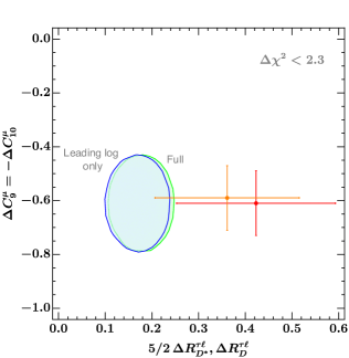
Figure 2: Model prediction for $\Delta C_{9}^{\mu}=-\Delta C_{10}^{\mu}$, $\Delta R_{D^{*}}^{\tau\ell}$, and $\Delta R_{D}^{\tau\ell}$ for the $\Delta\chi^{2}\leq 2.3~{}(1\sigma)$ fit region: in blue including only the logarithmic contribution in (28), and in green including also the non-logarithmic corrections. The $1\sigma$ experimental data are shown by the two crosses. Predictions and results for $\Delta R_{D^{*}}^{\tau\ell}$ (red cross) are scaled by $5/2$ compared to $\Delta R_{D}^{\tau\ell}$ (orange cross), since our model predicts $\Delta R_{D}^{\tau\ell}\approx 5/2\times\Delta R_{D^{*}}^{\tau\ell}$.

Low-energy constraints. The low-energy phenomenology of the model can be described in terms of $\{C_{U},\epsilon,\theta_{\tau\mu},\theta_{bs}\}$ and the discrete parameter $\theta_{LR}$. The list of relevant low-energy observables, with their explicit expression in terms of four-fermion effective operators, is given in Table II of Ref. Buttazzo:2017ixm . An important difference is the appearence of effective charged-current scalar operators from the right-handed terms in (23). These have a negligible impact in $B\to D^{*}\tau\nu$, but are non-negligible in $B\to D\tau\nu$. Using the results in Ref. Fajfer:2012vx for the matrix-elements of the $(\bar{b}_{R}c_{L})(\bar{\nu}_{L}\tau_{R})$ operator, we obtain in the limit $\theta_{\tau\mu},\theta_{bs}\to 0$

$$\begin{aligned} \Delta R_{D^{*}}^{\tau\ell}&=R_{D^{*}}^{\tau\ell}-1\approx 2[1-0.12\cos(\theta_{LR})]C_{U}~{},\\ \Delta R_{D}^{\tau\ell}&=R_{D}^{\tau\ell}-1\approx 2[1-1.5\cos(\theta_{LR})]C_{U}~{},\qquad\end{aligned}$$ (27)

with $R_{D^{(*)}}^{\tau\ell}$ defined as in Ref. Buttazzo:2017ixm . In order to maximize the correction to $R_{D^{(*)}}^{\tau\ell}$ we set $\theta_{LR}=\pi$. This implies the relation $\Delta R_{D}^{\tau\ell}\approx 5/2\times\Delta R_{D^{*}}^{\tau\ell}$, that is well consistent with present data Lees:2013uzd ; Aaij:2015yra ; Hirose:2016wfn ; Aaij:2017deq .

Having fixed $\theta_{LR}$, we determine the remaining four parameters from a global fit. At the best fit point we obtain $\chi^{2}_{\rm min}\approx 9$, which gives a very good fit compared to the SM, for which $\chi^{2}_{\rm SM}\approx 46$. A typical set of parameters providing a good fit to data is given by $C_{U}=0.03$, $\epsilon=-0.02$, $\theta_{\tau\mu}=-0.05$ and $\theta_{bs}=0.05\,V_{ts}$. This can be obtained for instance from the benchmark point: $g_{c}^{\mbox{\tiny($3$)}}=3$ and $M_{U_{3}}\approx 2$ TeV, with $M_{G^{\prime}}$ and $M_{Z^{\prime}}$ ranging between 1.5 and 3 TeV (depending on the $\omega_{1}/\omega_{3}$ ratio).

The potential of the model to explain the anomalies in $b\to s\ell\bar{\ell}$ (that we express as deviations in the Wilson coefficients $C_{9,10}$, defined as in Altmannshofer:2015sma ; Descotes-Genon:2015uva ) and in $R_{D^{(*)}}^{\tau\ell}$ (for which we adopt the updated SM prediction in Bigi:2017jbd ; Jaiswal:2017rve ; Bigi:2016mdz ) is depicted in Fig. 2. A good fit to $b\to s\ell\bar{\ell}$ data can only be achieved when considering the dimension-six operator (17), whose effect is encoded in $\epsilon$. Interestingly, the best fit value for $\epsilon$ is perfectly consistent with that of the dimension-six contributions in the Yukawa couplings.

While the model significantly reduces the tension with data, predicting a non-trivial correlation between $R_{D}^{\tau\ell}$ and $R_{D^{*}}^{\tau\ell}$ (see caption of Fig. 2), the central value of these two observables cannot be achieved due to the constraints from LFU tests in $\tau$ physics and $\mathcal{B}(B_{c,u}\to\tau\nu)$. The LFU tests yield per-mille constraints on the modifications of $W$ and $Z$ couplings to $\tau$ leptons ($\delta g_{\tau}^{W}$ and $\delta g^{Z}_{\tau_{L},\nu_{\tau}}$) EWPT . These quantities arise in our model from one-loop diagrams involving SM fermions and LQ fields Loop , whose (leading) result at $\mathcal{O}(y_{t}^{2})$ is

$$\begin{aligned} \delta g_{\tau}^{W}/g_{\ell}^{W}&=\frac{3\,y_{t}^{2}}{16\pi^{2}}\,C_{U}\left(\frac{1}{2}+\log\frac{m_{t}^{2}}{M_{U}^{2}}\right)\,,\\ \delta g^{Z}_{\nu_{\tau}}/g^{Z}_{\nu_{\ell}}&=\frac{3\,y_{t}^{2}}{8\pi^{2}}\,C_{U}\left(1+\log\frac{m_{t}^{2}}{M_{U}^{2}}\right)\,.\end{aligned}$$ (28)

These expressions agree in the logarithmic part with the EFT results in Jenkins:2013wua ; Feruglio:2016gvd ; Feruglio:2017rjo . However, having a complete model, we have been able to compute also the non-logarithmic terms which are non-negligible and partially alleviate the tensions with LFU tests in $\tau$ physics (see Fig. 2). As far as $\mathcal{B}(B_{c,u}\to\tau\nu)$ are concerned, at the best fit point we predict a $\sim 60\%$ enhancement over the SM, which is perfectly consistent with present data.

Another important constraint is obtained from $B_{s,d}$ mixing. Contributions to these observables arise in our model from the tree-level exchange of the coloron and the $Z^{\prime}$, as well as from one-loop box diagrams involving the vector leptoquark. All these contributions are proportional to the down-type rotation angle $|\theta_{bs}|$. Allowing for ($U(2)^{5}$ preserving) deviations of up to $\mathcal{O}(10\%)$ in $B_{s,d}$ mixing leads to the bound $|\theta_{bs}|\lesssim 0.1\,|V_{ts}|$, forcing a flavor-alignment in the down-quark sector. As a result of this alignment, contributions to $D-\bar{D}$ mixing from coloron and $Z^{\prime}$ exchange turn out to be below the present limits and do not give any relevant bound.

The vector leptoquark does not contribute significantly to $B\to K^{(*)}\nu\bar{\nu}$ nor to $\tau\to 3\mu$, while the approximate down-alignment in the quark sector required from $B_{s}$ mixing renders the $Z^{\prime}$ contribution to $B\to K^{(*)}\nu\bar{\nu}$ negligibly small. The $Z^{\prime}$ contributes at tree-level to $\tau\to 3\mu$. However, since its coupling to muons is suppressed, the constraints from these processes only become relevant when the leptonic mixing angle $\theta_{\tau\mu}$ becomes large, effectively setting the bound $|\theta_{\tau\mu}|\lesssim 0.1$.

High-$p_{T}$ searches. The masses of the lightest exotic vector bosons predicted by the model are expected to lie around the TeV scale, and are therefore constrained by direct searches at LHC. The phenomenology for these searches is very similar to the one discussed in the model of Ref. DiLuzio:2017vat , so we only highlight the main aspects.

$\bullet$ $U$. The vector LQ is subject to the bounds coming from QCD pair production and from tau pair production at high-energies (i.e. $pp\to\tau\bar{\tau}+X$), generated by $t$–channel exchange Faroughy:2016osc . As in Ref. DiLuzio:2017vat , the most stringent constraint is set by leptoquark pair production, which implies $M_{U}\gtrsim 1.3$ TeV. This expression is obtained by recasting DiLuzio:2017chi the CMS search in Ref. Sirunyan:2017yrk and translates to $C_{U}\lesssim 0.08$ for $g_{c}^{\mbox{\tiny($3$)}}=3$.

$\bullet$ $G^{\prime}$. Given the large couplings and relatively low mass of the coloron, di-jet searches at LHC can offer an important test of the validity of the model. However, current limits Aaboud:2017yvp rely on bump searches that become less sensitive when the coloron width is large. This is the case in our model, where we find $\Gamma_{G^{\prime}}/M_{G^{\prime}}=0.22$ for $g_{c}^{\mbox{\tiny($3$)}}=3$, if we assume that the only available decay channels are those to SM quarks. For large widths, the coloron signal is diluted into the QCD background allowing the model to avoid current bounds Admir:implications .

$\bullet$ $Z^{\prime}$. As already mentioned, the $Z^{\prime}$ couplings to light generations appear strongly suppressed compared to the third-generation ones. This renders the $Z^{\prime}$ Drell-Yan production at LHC sufficiently small to evade the strong bounds from di-lepton resonance searches Aaboud:2017buh .

$\bullet$ Heavy scalars. The minimal model discussed in Section II.3 presents a rich scalar sector, whose phenomenological analysis depends significantly on the details of the scalar potential and is beyond the scope of the present letter. Nevertheless, we do not expect it to yield tensions with data in large areas of the parameter space.

IV Summary and conclusions

If unambiguously confirmed as beyond-the-SM signals, the recent $B$-physics anomalies would lead to a significant shift in our understanding of fundamental interactions. They could imply abandoning the assumption of flavor universality of gauge interactions, which implicitly holds in the SM and in its most popular extensions. In this paper we have presented a model where the idea of flavor non-universal gauge interactions is pushed to its extreme consequences, with an independent gauge group for each fermion family.

The idea of the (flavor-blind) SM gauge group being the result of a suitable breaking of a flavor non-universal gauge symmetry, holding at high energies, has already been proposed in the past as a possible explanation for the observed flavor hierarchies (see e.g. Craig:2011yk ; Barbieri:2011ci ). Interestingly, constructions of this type naturally arise in higher-dimensional models (see e.g. Honecker:2003vq ) with fermion fields localized on different four-dimensional branes, the multi-site gauge group being the deconstructed version of a single higher-dimensional gauge symmetry ArkaniHamed:2001nc .

As we have shown in this paper, a three-site Pati-Salam gauge symmetry, with a suitable symmetry breaking sector, could describe in a natural way the observed Yukawa hierarchies and explain at the same time the recent $B$-physics anomalies, while being consistent with the tight constraints from other low- and high-energy measurements. The model we present exhibits a rich TeV-scale phenomenology that can be probed in the near future by high-$p_{T}$ experiments at the LHC.

- (1) J. P. Lees et al. [BaBar Collaboration], Phys. Rev. D 88 (2013) no.7, 072012 [arXiv:1303.0571].
- (2) R. Aaij et al. [LHCb Collaboration], Phys. Rev. Lett. 115 (2015) no.11, 111803 Erratum: [Phys. Rev. Lett. 115 (2015) no.15, 159901] [arXiv:1506.08614].
- (3) S. Hirose et al. [Belle Collaboration], Phys. Rev. Lett. 118 (2017) no.21, 211801 [arXiv:1612.00529].
- (4) R. Aaij et al. [LHCb Collaboration], [arXiv:1711.02505].
- (5) R. Aaij et al. [LHCb Collaboration], Phys. Rev. Lett. 113 (2014) 151601 [arXiv:1406.6482].
- (6) R. Aaij et al. [LHCb Collaboration], JHEP 1708 (2017) 055 [arXiv:1705.05802].
- (7) W. Altmannshofer and D. M. Straub, [arXiv:1503.06199].
- (8) S. Descotes-Genon, L. Hofer, J. Matias and J. Virto, JHEP 1606 (2016) 092 [arXiv:1510.04239].
- (9) R. Aaij et al. [LHCb Collaboration], Phys. Rev. Lett. 111 (2013) 191801 [arXiv:1308.1707].
- (10) R. Aaij et al. [LHCb Collaboration], JHEP 1602 (2016) 104 [arXiv:1512.04442].
- (11) B. Bhattacharya, A. Datta, D. London and S. Shivashankara, Phys. Lett. B 742 (2015) 370 [arXiv:1412.7164].
- (12) R. Alonso, B. Grinstein and J. Martin Camalich, JHEP 1510 (2015) 184 [arXiv:1505.05164].
- (13) A. Greljo, G. Isidori and D. Marzocca, JHEP 1507 (2015) 142 [arXiv:1506.01705].
- (14) L. Calibbi, A. Crivellin and T. Ota, Phys. Rev. Lett. 115 (2015) 181801 [arXiv:1506.02661].
- (15) M. Bauer and M. Neubert, Phys. Rev. Lett. 116 (2016) no.14, 141802 [arXiv:1511.01900].
- (16) S. Fajfer and N. Košnik, Phys. Lett. B 755 (2016) 270 [arXiv:1511.06024].
- (17) R. Barbieri, G. Isidori, A. Pattori and F. Senia, Eur. Phys. J. C 76 (2016) no.2, 67 [arXiv:1512.01560].
- (18) S. M. Boucenna, A. Celis, J. Fuentes-Martin, A. Vicente and J. Virto, Phys. Lett. B 760 (2016) 214 [arXiv:1604.03088].
- (19) D. Buttazzo, A. Greljo, G. Isidori and D. Marzocca, JHEP 1608 (2016) 035 [arXiv:1604.03940].
- (20) D. Das, C. Hati, G. Kumar and N. Mahajan, Phys. Rev. D 94 (2016) 055034 [arXiv:1605.06313].
- (21) S. M. Boucenna, A. Celis, J. Fuentes-Martin, A. Vicente and J. Virto, JHEP 1612 (2016) 059 [arXiv:1608.01349].
- (22) D. Bečirević, N. Košnik, O. Sumensari and R. Zukanovich Funchal, JHEP 1611 (2016) 035 [arXiv:1608.07583].
- (23) G. Hiller, D. Loose and K. Schönwald, JHEP 1612 (2016) 027 [arXiv:1609.08895].
- (24) B. Bhattacharya, A. Datta, J. P. Guévin, D. London and R. Watanabe, JHEP 1701 (2017) 015 [arXiv:1609.09078].
- (25) R. Barbieri, C. W. Murphy and F. Senia, Eur. Phys. J. C 77 (2017) no.1, 8 [arXiv:1611.04930].
- (26) M. Bordone, G. Isidori and S. Trifinopoulos, Phys. Rev. D 96 (2017) no.1, 015038 [arXiv:1702.07238].
- (27) E. Megias, M. Quiros and L. Salas, JHEP 1707 (2017) 102 [arXiv:1703.06019].
- (28) A. Crivellin, D. Müller and T. Ota, JHEP 1709 (2017) 040 [arXiv:1703.09226].
- (29) Y. Cai, J. Gargalionis, M. A. Schmidt and R. R. Volkas, JHEP 1710 (2017) 047 [arXiv:1704.05849].
- (30) R. Barbieri, G. Isidori, J. Jones-Perez, P. Lodone and D. M. Straub, Eur. Phys. J. C 71 (2011) 1725 [arXiv:1105.2296].
- (31) D. Buttazzo, A. Greljo, G. Isidori and D. Marzocca, JHEP 1711 (2017) 044 [arXiv:1706.07808].
- (32) F. Feruglio, P. Paradisi and A. Pattori, JHEP 1709 (2017) 061 [arXiv:1705.00929].
- (33) F. Feruglio, P. Paradisi and A. Pattori, Phys. Rev. Lett. 118 (2017) no.1, 011801 [arXiv:1606.00524].
- (34) D. A. Faroughy, A. Greljo and J. F. Kamenik, Phys. Lett. B 764 (2017) 126 [arXiv:1609.07138].
- (35) N. Assad, B. Fornal and B. Grinstein, [arXiv:1708.06350].
- (36) L. Di Luzio, A. Greljo and M. Nardecchia, [arXiv:1708.08450].
- (37) L. Calibbi, A. Crivellin and T. Li, [arXiv:1709.00692].
- (38) J. C. Pati and A. Salam, Phys. Rev. D 10 (1974) 275 Erratum: [Phys. Rev. D 11 (1975) 703].
- (39) At mass terms for the right-handed neutrinos of the first two generations are allowed. We thus integrate out also remaining with 5 independent species of massless fermions charged under .
- (40) G. Isidori, [arXiv:1302.0661].
- (41) G. F. Giudice, G. Isidori, A. Salvio and A. Strumia, JHEP 1502 (2015) 137 [arXiv:1412.2769].
- (42) B. Grzadkowski, M. Iskrzynski, M. Misiak and J. Rosiek, JHEP 1010 (2010) 085 [arXiv:1008.4884].
- (43) S. Fajfer, J. F. Kamenik and I. Nisandzic, Phys. Rev. D 85 (2012) 094025 [arXiv:1203.2654].
- (44) D. Bigi, P. Gambino and S. Schacht, JHEP 1711 (2017) 061 [arXiv:1707.09509].
- (45) S. Jaiswal, S. Nandi and S. K. Patra, JHEP 1712 (2017) 060 [arXiv:1707.09977 [hep-ph]].
- (46) D. Bigi and P. Gambino, Phys. Rev. D 94 (2016) no.9, 094008 [arXiv:1606.08030 [hep-ph]].
- (47) The dominant constrain arises from the bound on , for which we use the value reported in Y. Amhis et al., [arXiv:1612.07233].
- (48) An additional contribution to arises in our model from the mixing of the lowest-lying and the SM ; however, this receives a parametric suppression of and turns out to be negligible.
- (49) E. E. Jenkins, A. V. Manohar and M. Trott, JHEP 1401 (2014) 035 [arXiv:1310.4838].
- (50) L. Di Luzio and M. Nardecchia, Eur. Phys. J. C 77 (2017) no.8, 536 [arXiv:1706.01868].
- (51) A. M. Sirunyan et al. [CMS Collaboration], JHEP 1707 (2017) 121 [arXiv:1703.03995].
- (52) M. Aaboud et al. [ATLAS Collaboration], Phys. Rev. D 96 (2017) no.5, 052004 [arXiv:1703.09127].
- (53) A. Greljo, Talk at Implications of LHCb measurements and future prospects 2017.
- (54) M. Aaboud et al. [ATLAS Collaboration], JHEP 1710 (2017) 182 [arXiv:1707.02424].
- (55) N. Craig, D. Green and A. Katz, JHEP 1107 (2011) 045 [arXiv:1103.3708].
- (56) R. Blumenhagen, L. Gorlich and T. Ott, JHEP 0301 (2003) 021 [hep-th/0211059]; G. Honecker, Nucl. Phys. B 666 (2003) 175 [hep-th/0303015].
- (57) N. Arkani-Hamed, A. G. Cohen and H. Georgi, Phys. Lett. B 513 (2001) 232 [hep-ph/0105239].