Dynamical phase transitions at finite temperature from fidelity and interferometric Loschmidt echo induced metrics

Abstract

We study finite-temperature Dynamical Quantum Phase Transitions (DQPTs) by means of the fidelity and the interferometric Loschmidt Echo (LE) induced metrics. We analyse the associated dynamical susceptibilities (Riemannian metrics), and derive analytic expressions for the case of two-band Hamiltonians. At zero temperature the two quantities are identical, nevertheless, at finite temperatures they behave very differently. Using the fidelity LE, the zero temperature DQPTs are gradually washed away with temperature, while the interferometric counterpart exhibits finite-temperature Phase Transitions (PTs). We analyse the physical differences between the two finite-temperature LE generalisations, and argue that, while the interferometric one is more sensitive and can therefore provide more information when applied to genuine quantum (microscopic) systems, when analysing many-body macroscopic systems, the fidelity-based counterpart is a more suitable quantity to study. Finally, we apply the previous results to two representative models of topological insulators in 1D and 2D.

I Introduction

Equilibrium Phase Transitions (PTs) are characterised by a non-analytic behaviour of relevant thermodynamic observables with respect to the change of temperature. Quantum Phase Transitions (QPTs) sac:07 , traditionally described by Landau theory lan:37 , occur when we adiabatically change a physical parameter of the system at zero temperature, i.e., the transition is driven by purely quantum fluctuations. A particularly interesting case arises when one studies QPTs in the context of topological phases of matter wen:90 ; kos:tho:72 ; kos:tho:73 ; hal:83 ; hal:88 . They are quite different from the standard QPTs, since they do not involve symmetry breaking and are characterised by global order parameters tknn:82 . These novel phases of matter, which include topological insulators and superconductors has:kan:10 ; qi:zha:11 ; ber:hug:13 , have potentially many applications in emerging fields such as spintronics, photonics or quantum computing. Although many of their remarkable properties have traditionally been studied at zero temperature, there has been a great effort to generalise these phases from pure to mixed states, and finite temperatures bar:waw:alt:flei:die:17 ; grus:17 ; mer:vla:pau:vie:17 ; mer:vla:pau:vie:17:qw ; sjo:15 ; viy:riv:mar:15 ; nie:hub:14 ; viy:riv:del:14 ; viy:riv:del:2d:14 ; bar:bar:krau:rico:ima:zol:die:13 ; riv:viy:del:13 ; viy:riv:del:12 ; viy:riv:gas:wal:fil:del:18 .

The real time evolution of closed quantum systems out of equilibrium has some surprising similarities with thermal phase transitions, as noticed by Heyl, Polkovnikov and Kehrein hey:pol:keh:13 . They coined the term Dynamical Quantum Phase Transitions (DQPTs) to describe the non-analytic behaviour of certain dynamical observables after a sudden quench in one of the parameters of the Hamiltonian. Since then, the study of DQPTs became an active field of research and a lot of progress has been achieved in comparing and connecting them to the equilibrium PTs kar:sch:13 ; and:sir:14 ; vaj:dor:14 ; hey:15 ; kar:sch:17 ; hal:zau:17 ; zau:hal:17 ; hom:abe:zau:hal:17 . Along those lines, there exist several studies of DQPTs for systems featuring non-trivial topological properties vaj:dor:15 ; sch:keh:15 ; bud:hey:16 ; hua:bal:16 ; jaf:joh:17 ; sed:flei:sir:17 . DQPTs have been experimentally observed in systems of trapped ions jur:etal:17 and cold atoms in optical lattices fla:etal:16. The figure of merit in the study of DQPTs is the Loschmidt Echo (LE) and its derivatives, which have been extensively used in the analysis of quantum criticality qua:son:liu:zan:sun:06 ; zan:pau:06 ; zan:qua:wan:sun:07 ; pol:muk:gre:moo:10 ; jac:ven:zan:11 and quantum quenches ven:zan:10 . At finite temperature, generalisations of the zero temperature LE were proposed, based on the mixed-state Uhlmann fidelity ven:tac:san:san:11 ; jac:ven:zan:11 , and the interferometric mixed-state geometric phase hey:bud:17 ; bah:ban:dut:17 . For an alternative approach to finite-temperature DPTs, see lan:fra:hal:17 ; hal:zau:mcc:veg:sch:kas:17 . Fidelity is a measure of state distinguishability, which has been employed numerous times in the study of PTs zan:pau:06 ; pau:sac:nog:vie:dug ; zan:ven:gio:07 ; aba:ham:zan:08 ; zha:zho:09 , while the interferometric mixed-state geometric phase was introduced in sjo:pat:eke:ana:eri:oi:ved:00 . The two quantities are in general different and it comes as no surprise that they give different predictions for the finite temperature behaviour bah:ban:dut:17 : the fidelity LE does not show DPTs at finite temperatures, while the interferometric LE indicates their persistence at finite temperature. Thus, it remains unclear what the fate of DQPT at finite temperature truly is, and which of the two opposite predictions better captures the many-body nature of these PTs.

In this paper, we discuss the existence of finite temperature Dynamical Phase Transitions (DPTs) for the broad class of two-band Hamiltonians in terms of both the fidelity and the interferometric LEs. We derive analytic expressions for the metrics (susceptibilities) induced by the fidelity and the interferometric LEs, respectively, showing explicitly that the two approaches give different behaviours: the fidelity susceptibility shows a gradual disappearance of DPTs as the temperature increases, while the interferometric susceptibility indicates their persistence at finite temperature (consistent with recent studies on interferometric LE hey:bud:17 ; bah:ban:dut:17 ). We analyze the reasons for such different behaviours. The fidelity LE quantifies state distinguishability in terms of measurements of physical properties, inducing a metric over the space of quantum states, while the interferometric LE quantifies the effects of quantum channels acting upon a state, inducing a pullback metric over the space of unitaries. Thus, we argue that the fidelity LE and its associated dynamical susceptibility are more suitable for the study of many-body systems, while the more sensitive interferometric counterparts are optimal when considering genuine microscopic quantum systems. In addition, interferometric experiments that are suitable for genuine (microscopic) quantum systems involve coherent superpositions of two states, which could be, in the case of many-body macroscopic systems, experimentally infeasible with current technology. To confirm our analysis for the fidelity LE, we also present quantitative results for the fidelity-induced first time derivative of the rate function in the case of the 1D Su-Schrieffer-Heeger (SSH) topological insulator and the 2D Massive Dirac (MD) model of a Chern insulator qi:hug:zha:08 .

II Dynamical (quantum) phase transitions and associated susceptibilities

The authors in hey:pol:keh:13 introduce the concept of DQPTs and illustrate their properties on the case of the transverse-field Ising model. They observe a similarity between the partition function of a quantum system in equilibrium, $Z(\beta)=\text{Tr}(e^{-\beta H})$, and the overlap amplitude of some time-evolved initial quantum state $|\psi_{i}\rangle$ with itself, $G(t)=\langle\psi_{i}|e^{-iHt}|\psi_{i}\rangle$. During a temperature-driven PT, the abrupt change of the properties of the system is indicated by the non-analyticity of the free energy density $f(\beta)=-\lim_{N\to\infty}\frac{1}{N}\ln Z(\beta)$ at the critical temperature ($N$ being the number of degrees of freedom). It is then possible to establish an analogy with the case of the real time evolution of a quantum system out of equilibrium, by considering the rate function

$$g(t)=-\frac{1}{N}\log|G(t)|^{2},$$ (1)

where $|G(t)|^{2}$ is a mixed-state LE, as we detail below. The rate function $g(t)$ may exhibit non-analyticities at some critical times $t_{c}$, after a quantum quench. This phenomenon is termed DPT.

We study DPTs for mixed states using the fidelity and the interferometric LEs. We first investigate the relation between the two approaches for DQPTs at zero temperature. More concretely, we perform analytical derivations of the corresponding susceptibilities in the general case of a family of static Hamiltonians, parametrised by some smooth manifold $M$, $\{H(\lambda):\lambda\in M\}$.

II.1 DQPTs for pure states

At zero temperature, the LE $G(t)$ from (1) between the ground state for $\lambda=\lambda_{i}\in M$ and the evolved state with respect to the Hamiltonian for $\lambda=\lambda_{f}\in M$ is given by the fidelity between the two states

$$\mathcal{F}(t;\lambda_{f},\lambda_{i})\equiv|\langle\psi(\lambda_{i})|e^{-itH(\lambda_{f})}|\psi(\lambda_{i})\rangle|.$$ (2)

For $\lambda_{i}=\lambda_{f}$, the fidelity is trivial, since the system remains in the same state. Fixing $\lambda_{i}\equiv\lambda$ and $\lambda_{f}=\lambda+\delta\lambda$, with $\delta\lambda<<1$, in the $t\rightarrow\infty$ limit Eq. (2) is nothing but the familiar $S$-matrix with an unperturbed Hamiltonian $H(\lambda)$ and an interaction Hamiltonian $V(\lambda)$, which is approximated by

$$V(\lambda)\equiv H(\lambda_{f})-H(\lambda)\approx\frac{\partial H}{\partial\lambda^{a}}(\lambda)\delta\lambda^{a}.$$ (3)

After applying standard perturbation theory techniques (for details, see Appendix), we obtain

$$\mathcal{F}(t;\lambda_{f},\lambda)\approx 1-\chi_{ab}(t;\lambda)\delta\lambda^{a}\delta\lambda^{b},$$ (4)

where the dynamical susceptibility $\chi_{ab}(t;\lambda)$ is given by

$$\chi_{ab}(t;\lambda)=\int_{0}^{t}\int_{0}^{t}dt_{2}dt_{1}\left(\frac{1}{2}\langle\{V_{a}(t_{2}),V_{b}(t_{1})\}\rangle-\langle V_{a}(t_{2})\rangle\langle V_{b}(t_{1})\rangle\right),$$ (5)

with $V_{a}(t,\lambda)=e^{itH(\lambda)}\partial H/\partial\lambda^{a}(\lambda)e^{-itH(\lambda)}$ and $\langle\ast\rangle=\langle\psi(\lambda)|\ast|\psi(\lambda)\rangle$. The family of symmetric tensors $\{ds^{2}(t)=\chi_{ab}(t,\lambda)d\lambda^{a}d\lambda^{b}\}_{t\in\mathbb{R}}$ defines a family of metrics in the manifold $M$, which can be seen as pullback metrics of the Bures metric (Fubini-Study metric) in the manifold of pure states chr:jam:12 . Specifically, at time $t$, the pullback is given by the map $\Phi_{t}:\lambda_{f}\mapsto e^{-itH(\lambda_{f})}|\psi(\lambda)\rangle\langle\psi(\lambda)|e^{itH(\lambda_{f})}$, evaluated at $\lambda_{f}=\lambda$.

II.2 Generalizations at finite temperatures

The generalization of DQPTs to mixed states is not unique. There are several ways to construct a LE for a general density matrix. In what follows, we derive two finite temperature generalizations, such that they have the same zero temperature limit.

II.2.1 Fidelity Loschmidt Echo at $T>0$

First, we introduce the fidelity LE between the state $\rho(\beta;\lambda_{i})=e^{-\beta H(\lambda_{i})}/\text{Tr}\{e^{-\beta H(\lambda_{i})}\}$ and the one evolved by the unitary operator $e^{-itH(\lambda_{f})}$ as

$$\!\!\!\!\!\!\mathcal{F}(t,\beta;\lambda_{i},\lambda_{f})\!=\!F(\rho(\beta;\lambda_{i}),e^{-itH(\lambda_{f})}\rho(\beta;\lambda_{i})e^{itH(\lambda_{f})}),$$ (6)

where $F(\rho,\sigma)=\text{Tr}\{\sqrt{\sqrt{\rho}\sigma\sqrt{\rho}}\}$ is the quantum fidelity between arbitrary mixed states $\rho$ and $\sigma$. For $\lambda_{f}$ close to $\lambda_{i}=\lambda$, we can write

$$\mathcal{F}(t,\beta;\lambda_{f},\lambda)\approx 1-\chi_{ab}(t,\beta;\lambda)\delta\lambda^{a}\delta\lambda^{b},$$ (7)

with $\chi_{ab}(t,\beta,\lambda)$ being the Dynamical Fidelity Susceptibility (DFS). Notice that $\lim_{\beta\to\infty}\chi_{ab}(t,\beta;\lambda)=\chi_{ab}(t;\lambda)$, where $\chi_{ab}(t;\lambda)$ is given by Eq. (5). At time $t$ and inverse temperature $\beta$, we have a map $\Phi_{(t,\beta)}:\lambda_{f}\mapsto e^{-itH(\lambda_{f})}\rho(\beta;\lambda)e^{itH(\lambda_{f})}$. The $2$-parameter family of metrics defined by $ds^{2}(\beta,t)=\chi_{ab}(t,\beta;\lambda)d\lambda^{a}d\lambda^{b}$ is the pullback by $\Phi_{(t,\beta)}$ of the Bures metric on the manifold of full-rank density operators, evaluated at $\lambda_{f}=\lambda$ (see Appendix).

The fidelity LE is closely related to the Uhlmann connection: $F(\rho_{1},\rho_{2})$ equals the overlap between purifications $W_{1}$ and $W_{2}$, $\langle W_{1},W_{2}\rangle=\text{Tr}\left\{W_{1}^{\dagger}W_{2}\right\}$, satisfying discrete parallel transport condition (see, for instance uhl:11 ).

II.2.2 Interferometric Loschmidt Echo at $T>0$

Here, we consider an alternative definition of the LE for mixed states [$G(t)$ from Eq. (1)]. In particular, we define the interferometric LE as

$$\mathcal{L}(t,\beta;\lambda_{f},\lambda_{i})=\left|\frac{\text{Tr}\left\{e^{-\beta H(\lambda_{i})}e^{itH(\lambda_{i})}e^{-itH(\lambda_{f})}\right\}}{\text{Tr}\left\{e^{-\beta H(\lambda_{i})}\right\}}\right|.$$ (8)

The $e^{itH(\lambda_{i})}$ factor does not appear at zero temperature, since it just gives a phase which is canceled by taking the absolute value. This differs from previous treatments in the literature bud:hey:16 (see Section 5.5.4 of chr:jam:12 , where the variation of the interferometric phase, $\text{Tr}\{\rho_{0}e^{-itH}\}$, exposes this structure). However, it is convenient to introduce it in order to have the usual form of the perturbation expansion, as will become clear later.

For $\lambda_{f}$ close to $\lambda_{i}=\lambda$, we get

$$\mathcal{L}(t,\beta;\lambda_{f},\lambda)\approx\left|\frac{\text{Tr}\left\{e^{-\beta H(\lambda)}Te^{-i\int_{0}^{t}dt^{\prime}V_{a}(t,\lambda)\delta\lambda^{a}}\right\}}{\text{Tr}\left\{e^{-\beta H(\lambda)}\right\}}\right|,$$ (9)

so that the perturbation expansion goes as in Eq. (5), yielding

$$\mathcal{L}(t,\beta;\lambda_{f},\lambda)\approx 1-\tilde{\chi}_{ab}(t,\beta;\lambda)\delta\lambda^{a}\delta\lambda^{b},$$ (10)

with the dynamical susceptibility given by

$$\tilde{\chi}_{ab}(t,\beta;\lambda)=\int_{0}^{t}\int_{0}^{t}dt_{2}dt_{1}\left(\frac{1}{2}\langle\{V_{a}(t_{2}),V_{b}(t_{1})\}\rangle-\langle V_{a}(t_{2})\rangle\langle V_{b}(t_{1})\rangle\right),$$ (11)

where $\langle\ast\rangle=\text{Tr}\{e^{-\beta H(\lambda)}\ast\}/\text{Tr}\{e^{-\beta H(\lambda)}\}$. Notice that Eqs (11) and (5) are formally the same with the average over the ground state replaced by the thermal average. This justifies the extra $e^{itH(\lambda_{i})}$ factor. Since this susceptibility comes from the interferometric LE, we call it Dynamical Interferometric Susceptibility (DIS). The quantity $ds^{2}(\beta,t)=\tilde{\chi}_{ab}(t,\beta;\lambda)d\lambda^{a}d\lambda^{b}$ defines a $2$-parameter family of metrics over the manifold $M$, except that they cannot be seen as pullbacks of metrics on the manifold of density operators with full rank. However, it can be interpreted as the pullback by a map from $M$ to the unitary group associated with the Hilbert space of a particular Riemannian metric. For a detailed analysis, see Appendix. Additionally, we point out that this version of LE is related to the interferometric geometric phase introduced by Sjöqvist et. al sjo:pat:eke:ana:eri:oi:ved:00 ; ton:sjo:kwe:oh .

II.3 Two-band systems

Many representative examples of topological insulators and superconductors can be described by effective two-band Hamiltonians. Therefore, we derive closed expressions of the previously introduced dynamical susceptibilities for topological systems within this class.

The general form of such Hamiltonians is $\{H(\lambda)=\vec{x}(\lambda)\cdot\vec{\sigma}:\lambda\in M\}$, where $\vec{\sigma}$ is the Pauli vector. The interaction Hamiltonian $V(\lambda)$, introduced in Eq. (2), casts the form

$$V(\lambda)\approx\left(\frac{\partial\vec{x}}{\partial\lambda^{a}}\cdot\vec{\sigma}\right)\delta\lambda^{a}.$$

It is convenient to decompose $\partial\vec{x}/\partial\lambda^{a}$ into one component perpendicular to $\vec{x}$ and one parallel to it:

$$\frac{\partial\vec{x}}{\partial\lambda^{a}}=\left(\frac{\partial\vec{x}}{\partial\lambda^{a}}\right)^{\perp}+\left(\frac{\partial\vec{x}}{\partial\lambda^{a}}\right)^{\parallel}=\vec{t}_{a}+\vec{n}_{a}.$$

The first term is tangent, in $\mathbb{R}^{3}$, at $\vec{x}(\lambda)$, to a sphere of constant radius $r=|\vec{x}(\lambda)|$. Hence, this kind of perturbations does not change the spectrum of $H$, only its eigenbasis. The second term is a variation of the length of $\vec{x}$ and hence, it changes the spectrum of $H$, while keeping the eigenbasis fixed. The DFS and the DIS are given by (for the details of the derivation, see Appendix)

$$\chi_{ab} = \tanh^{2}(\beta|\vec{x}(\lambda)|)\frac{\sin^{2}(|\vec{x}(\lambda)|t)}{|\vec{x}(\lambda)|^{2}}\vec{t}_{a}\!\!\cdot\!\vec{t}_{b}$$ (12)

$$\tilde{\chi}_{ab}\! = \!\frac{\sin^{2}(|\vec{x}(\lambda)|t)}{|\vec{x}(\lambda)|^{2}}\vec{t}_{a}\!\!\cdot\!\vec{t}_{b}\!+\!t^{2}(1\!\!-\!\!\tanh^{2}(\beta|\vec{x}(\lambda)|))\vec{n}_{a}\!\!\!\cdot\!\vec{n}_{b}.$$ (13)

While the DIS (13) depends on the variation of both the spectrum and the eigenbasis of the Hamiltonian, the DFS (12) depends only on the variations which preserve the spectrum, i.e., changes in the eigenbasis. This is very remarkable, in general the fidelity between two quantum states, being their distinguishability measure, does depend on both the variations of the spectrum and the eigenbasis. In our particular case of a quenched system, the eigenvalues are preserved (see Eq. (6)), as the system is subject to a unitary evolution. The tangential components of both susceptibilities are modulated by the function $\sin^{2}(Et)/E^{2}$, where $E$ is the gap. This captures the Fisher zeros, i.e., the zeros of the (dynamical) partition function which here is given by the fidelity $\mathcal{F}$ from (6) (see yan:lee:52 ; lee:yan:52 ; fis:65 ). Observe that whenever $t=(2n+1)\pi/2E$, $n\in\mathbb{Z}$, this factor is maximal and hence, both LEs decrease abruptly. The difference between the two susceptibilities is given by

$$\tilde{\chi}_{ab}-\chi_{ab}=(1-\tanh^{2}(\beta|\vec{x}(\lambda)|))\left(\frac{\sin^{2}(|\vec{x}(\lambda)|t)}{|\vec{x}(\lambda)|^{2}}\vec{t}_{a}\cdot\vec{t}_{b}+t^{2}\vec{n}_{a}\cdot\vec{n}_{b}\right).$$

The quantity $(1-\tanh^{2}(\beta E))$ is nothing but the static susceptibility, see pat:96 . Therefore, the difference between DIS and DFS is modulated by the static susceptibility at finite temperature.

To illustrate the relationship between the two susceptibilities, in FIG. 1 we plotted the modulating function for the tangential components of both. We observe that at zero temperature they coincide. As the temperature increases, in the case of the fidelity LE, the gap-vanishing points become less important. On the contrary, for the interferometric LE, the associated tangential part of the susceptibility does not depend on temperature, thus the gap-vanishing points remain prominent. The DFS from Eq. (12) thus predicts gradual smearing of critical behaviour, consistent with previous findings that showed the absence of phase transitions at finite temperatures in the static case mer:vla:pau:vie:17 ; mer:vla:pau:vie:17:qw . The DIS from Eq.(13) has a tangential term that is not coupled to the temperature, persisting at higher temperatures and giving rise to abrupt changes in the finite-temperature system’s behaviour. This is also consistent with previous studies in the literature, where DPTs were found even at finite temperatures hey:bud:17 ; bah:ban:dut:17 . Additionally, the interferometric LE depends on the normal components of the variation of $\vec{x}$. In other words, the finite-temperature phase transitions inferred by the behavior of the interferometric LE occur due to the change of the parameters of the Hamiltonian and not due to temperature.

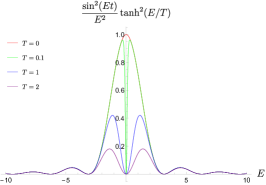
Figure 1: The susceptibility modulating function for the tangential components at $t=1$.

II.4 Comparing the two approaches

The above analysis of the two dynamical susceptibilities (metrics) reflects the essential difference between the two distinguishability measures, one based on the fidelity, the other on interferometric experiments. From the quantum information theoretical point of view, the two quantities can be interpreted as distances between states, or between processes, respectively. The Hamiltonian evaluated at a certain point of parameter space $M$ defines the macroscopic phase. Associated to it we have thermal states and unitary processes. The fidelity LE is obtained from the Bures distance between a thermal state $\rho_{1}$ in phase $1$ and the one obtained by unitarily evolving this state, $\rho_{2}=U_{2}\rho_{1}U_{2}^{\dagger}$, with $U_{2}$ associated to phase $2$. Given a thermal state $\rho_{1}$ prepared in phase $1$, the interferometric LE is obtained from the distance between two unitary processes $U_{1}$ and $U_{2}$ (defined modulo a phase factor), associated to phases $1$ and $2$.

The quantum fidelity between two states is in fact the classical fidelity between the probability distributions obtained by performing an optimal measurement on them. Measuring an observable $M$ on the two states $\rho_{1}$ and $\rho_{2}$, one obtains the probability distributions $\{p_{1}(i)\}$ and $\{p_{2}(i)\}$, respectively. The quantum fidelity $F_{Q}$ between the two states $\rho_{1}$ and $\rho_{2}$ is bounded by the classical fidelity $F_{C}$ between the probability distributions $\{p_{1}(i)\}$ and $\{p_{2}(i)\}$, $F_{Q}(\rho_{1},\rho_{2})=\mbox{Tr}\sqrt{\sqrt{\rho_{1}}\rho_{2}\sqrt{\rho_{1}}}\leq\sum_{i}\sqrt{p_{1}(i)p_{2}(i)=F_{c}(p_{1}(i),p_{2}(i))}$, such that the equality is obtained by measuring an optimal observable, given by $M_{\text{op}}=\rho_{1}^{-1/2}\sqrt{\sqrt{\rho_{1}}\rho_{2}\sqrt{\rho_{1}}}\rho_{1}^{-1/2}$ (note that optimal observable is not unique). For that reason, one can argue that the fidelity is capturing all order parameters (i.e., measurements) through its optimal observables $M_{\text{op}}$. Fidelity-induced distances, the Bures distance $D_{B}(\rho_{1},\rho_{2})=\sqrt{2(1-F_{Q}(\rho_{1},\rho_{2}))}$, the sine distance $D_{S}(\rho_{1},\rho_{2})=\sqrt{1-F_{Q}^{2}(\rho_{1},\rho_{2})}$ and the F-distance $D_{F}(\rho_{1},\rho_{2})=1-F_{Q}(\rho_{1},\rho_{2})$ satisfy the following set of inequalities

$$D_{F}(\rho_{1},\rho_{2})\leq D_{T}(\rho_{1},\rho_{2})\leq D_{S}(\rho_{1},\rho_{2})\leq D_{B}(\rho_{1},\rho_{2}),$$

where the trace distance is given by $D_{T}(\rho_{1},\rho_{2})=\frac{1}{2}\mbox{Tr}|\rho_{1}-\rho_{2}|$. In other words, the fidelity-induced distances and the trace distance establish the same order on the space of quantum states. This is important, as the trace distance is giving the optimal value for the success probability in ambiguously discriminating in a single-shot measurement between two a priori equally probable states $\rho_{1}$ and $\rho_{2}$, given by the so-called Helstrom bound $P_{H}(\rho_{1},\rho_{2})=(1+D_{T}(\rho_{1},\rho_{2}))/2$ hel:76 .

On the other hand, the interferometric phase is based on some interferometric experiment to distinguish two states, $\rho_{1}=\sum_{i}r_{i}|i\rangle\langle i|$ and $\rho_{2}=U_{2}\rho_{1}U_{2}^{\dagger}$: it measures how the intensities at the outputs of the interferometer are affected by applying $U_{2}$ to only one of its arms sjo:pat:eke:ana:eri:oi:ved:00 . Therefore, to set up such an experiment, one does not need to know the state $\rho_{1}$ that enters the interferometer, as only the knowledge of $U_{2}$ is required. Note that this does not mean that the output intensities do not depend on the interferometric LE: indeed, the inner product $\langle U_{1},U_{2}\rangle_{\rho_{1}}$ is defined with respect to the state $\rho_{1}$. This is a different type of experiment, not based on the observation of any physical property of a system. It is analogous to comparing two masses with weighing scales, which would show the same difference of $\Delta m=m_{1}-m_{2}$, regardless of how large the two masses $m_{1}$ and $m_{2}$ are. For that reason, interferometric distinguishability is more sensitive than the fidelity (fidelity depends on more information, not only how much the two states are different, but in what aspects this difference is observable). Indeed, the interferometric LE between $\rho_{1}$ and $\rho_{2}$ can be written as the overlap $L(\rho_{1},\rho_{2})=|\langle\rho_{1}|\rho_{2}\rangle|$ between the purifications $|\rho_{1}\rangle=\sum_{i}\sqrt{r_{i}}|i\rangle|i\rangle$ and $|\rho_{2}\rangle=(U\otimes I)|\rho_{1}\rangle$. On the other hand, the fidelity satisfies $F(\rho_{1},\rho_{2})=\max_{|\psi\rangle,|\varphi\rangle}|\langle\psi|\varphi\rangle|$, where $|\psi\rangle$ and $|\varphi\rangle$ are purifications of $\rho_{1}$ and $\rho_{2}$, respectively, i.e., $L(\rho_{1},\rho_{2})\leq F(\rho_{1},\rho_{2})$. Moreover, what one does observe in interferometric experiments are the mentioned output intensities, i.e., one needs a number of identical systems prepared in the same state to obtain results in interferometric measurements. This additionally explains why interferometric LE is more sensible than the fidelity one, as the latter is based on the observations performed on single systems. The fact that interferometric LE is more sensitive than the fidelity LE is consistent with the result that the former is able to capture the changes of some of the system’s features at finite temperatures (thus they predict DPTs), while the latter cannot.

In terms of experimental feasibility, the fidelity is more suitable for the study of many-body macroscopic systems and phenomena, while the interferometric measurements provide a more detailed information on genuinely quantum (microscopic) systems. Finally, interferometric experiments involve coherent superpositions of two states. Therefore, when applied to many-body systems, one would need to create genuine Schrödinger cat-like states, which goes beyond the current, and any foreseeable, technology (and could possibly be forbidden by more fundamental laws of physics; see for example objective collapse theories bas:loc:sat:sin:ulb:13 ).

III DPTs of topological insulators at finite temperatures

Our general study of two-band Hamiltonians showed that the fidelity-induced LE predicts a gradual smearing of DPTs with temperature. In order to test this result, we study the fidelity LE on concrete examples of two topological insulators (as noted in the main text, the analogous study for the interferometric LE on concrete examples has already been performed, and is consistent with our findings hey:bud:17 ; bah:ban:dut:17 ). In particular, we present quantitative results obtained for the first derivative of the rate function, $dg/dt$, where $g(t)=-\frac{1}{N}\log\mathcal{F}$, and

$$\!\!\!\!\!\!\mathcal{F}(t,\beta;\lambda_{i},\lambda_{f})\!=\!F(\rho(\beta;\lambda_{i}),e^{-itH(\lambda_{f})}\rho(\beta;\lambda_{i})e^{itH(\lambda_{f})}).$$

The fidelity $F$ is obtained by taking the product of the single-mode fidelities, each of which has the form

$$F(\rho(\beta;\lambda_{i}),e^{-itH(\lambda_{f})}\rho(\beta;\lambda_{i})e^{itH(\lambda_{f})})=\sqrt{\frac{1+\cosh^{2}(\beta E_{i})+\sinh^{2}(\beta E_{i})\left[\cos(2E_{f}t)+(1-\cos(2E_{f}t))(\vec{n}_{i}\cdot\vec{n}_{f})^{2})\right]}{2\cosh^{2}(\beta E_{i})}},$$

with $H_{a}=E_{a}\vec{n}_{a}\cdot\vec{\sigma}$ and $a=i,f$. This expression can be obtained by using Eq. (17) and the result found in the Supplemental Material of mer:vla:pau:vie:17 . The quantity $dg/dt$ is the figure of merit in the study of the DQPTs, therefore we present the respective results that confirm the previous study: the generalisation of the LE with respect to the fidelity shows the absence of finite temperature dynamical PTs. We consider two paradigmatic models of topological insulators, namely the SSH su:sch:hee:79 and the MD qi:hug:zha:08 models.

III.1 SSH model (1D)

The SSH model was introduced in su:sch:hee:79 to describe polyacetilene, and it was later found to describe diatomic polymers ric:mel:82 . In momentum space, the Hamiltonian for this model is of the form $H(k,m)=\vec{x}(k,m)\cdot\vec{\sigma},$ with $m$ being the parameter that drives the static PT. The vector $\vec{x}(k,m)$ is given by:

$$\vec{x}(k,m)=(m+\cos(k),\sin(k),0).$$

By varying $m$ we find two distinct topological regimes. For $m<m_{c}=1$ the system is in a non-trivial phase with winding number $1$, while for $m>m_{c}=1$ the system is in a topologically trivial phase with winding number $0$.

We consider both cases in which we go from a trivial to a topological phase and vice versa (FIGs 2 and 3, respectively). We notice that non-analyticities of the first derivative appear at zero temperature, and they are smeared out for higher temperatures.

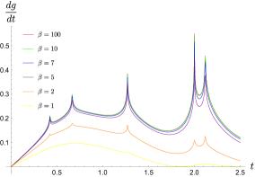
Figure 2: We plot the time derivative of the rate function, $dg/dt$, as a function of time for different values of the inverse temperature $\beta=1/T$. We consider a quantum quench from a trivial phase $(m=1.2)$ to a topological phase $(m=0.8)$.

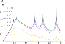
Figure 3: The time derivative of the rate function, $dg/dt$, as a function of time for different values of the inverse temperature. The quench is from a topological $(m=0.8)$ to a trivial phase $(m=1.2)$.

III.2 MD model (2D)

The Massive Dirac model (MDM) captures the physics of a 2D Chern insulator qi:hug:zha:08 , and shows different topologically distinct phases. In momentum space, the Hamiltonian for the MDM is of the form $H(\vec{k},m)=\vec{x}(\vec{k},m)\cdot\vec{\sigma},$ with $m$ being the parameter that drives the static PT. The vector $\vec{x}(\vec{k},m)$ is given by

$$\vec{x}(\vec{k},m)=(\sin(k_{x}),\sin(k_{y}),m-\cos(k_{x})-\cos(k_{y})).$$

By varying $m$ we find four different topological regimes:

• For $-\infty<m<m_{c_{1}}=-2$ it is trivial (the Chern number is zero) – Regime I

• For $-2=m_{c_{1}}<m<m_{c_{2}}=0$ it is topological (the Chern number is $-1$) – Regime II

• For $0=m_{c_{2}}<m<m_{c_{3}}=2$ it is topological (the Chern number is $+1$) – Regime III

• For $2=m_{c_{3}}<m<\infty$ it is trivial (the Chern number is zero) – Regime IV

In FIGs 4, 5 and 6 we plot the first derivative of the rate function $g(t)$, as a function of time for different temperatures. We only consider quenches that traverse a single phase transition point.

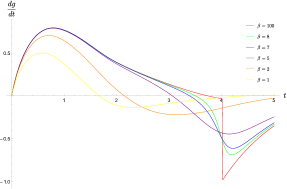
Figure 4: The time derivative of the rate function, $dg/dt$, as a function of time for different values of the inverse temperature. We quench the system from a trivial to a topological regime (Regimes from I to II and from IV to III).

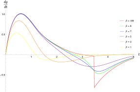
Figure 5: The time derivative of the rate function, $dg/dt$, as a function of time for different values of the inverse temperature. The quench is from a topological to a trivial regime (Regimes from II to I and from III to IV).

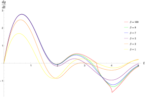
Figure 6: The time derivative of the rate function, $dg/dt$, as a function of time for different inverse temperatures. The quantum quench is from a topological to a topological regime (Regimes from II to III and vice versa).

We observe that at zero temperature there exist non-analyticities at the critical times – the signatures of DQPTs. As we increase the temperature, these non-analyticities are gradually smeared out, resulting in smooth curves for higher finite temperatures. We note that the peak of the derivative $dg(t)/dt$ is drifted when increasing the temperature, in analogy to the usual drift of non-dynamical quantum phase transitions at finite temperaturekem:que:smi:16 .

Next, we proceed by considering the cases in which we cross two phase transition points, as shown in FIGs 7 and 8. At zero temperature we obtain a non-analytic behaviour, which gradually disappears for higher temperatures.

Finally, we have also studied the case in which we move inside the same topological regime from left to right and vice versa. We obtained smooth curves without non – analyticities, which we omit for the sake of briefness.

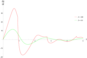
Figure 7: The time derivative of the rate function, $dg/dt$, as a function of time for different values of the inverse temperature, in the case that we quench the system from a trivial to a topological regime (Regimes from I to III and from IV to II).

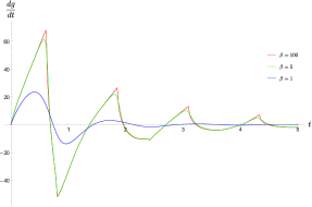
Figure 8: The time derivative of the rate function, $dg/dt$, as a function of time for different values of the inverse temperature. The system is quenched from a topological to a trivial regime (Regimes from III to I and from II to IV).

IV Conclusions

We analysed the fidelity and the interferometric generalisations of the LE for general mixed states, and applied them to the study of finite temperature DPTs in topological systems. We showed that the dynamical fidelity susceptibility is the pullback of the Bures metric in the space of density matrices, i.e., states. On the other hand, the dynamical interferometric susceptibility is the pullback of a metric in the space of unitaries (i.e., quantum channels).

The difference between the two metrics reflects the fact that the fidelity is a measure of the state distinguishability between two given states $\rho$ and $\sigma$ in terms of observations, while the “interferometric distinguishability” quantifies how a quantum channel (a unitary $U$) changes an arbitrary state $\rho$ to $U\rho U^{\dagger}$.

Therefore, while the “interferometric distinguishability” is in general more sensitive, and thus appropriate for the study of genuine (microscopic) systems, it is the fidelity that is the most suitable for the study of many-body system phases.

Moreover, interferometric experiments involve coherent superpositions of two states, which for many-body systems would require creating and manipulating genuine Schrödinger cat-like states. This seems to be experimentally beyond current technology.

We presented analytic expressions for the dynamical susceptibilities in the case of two-band Hamiltonians. At finite temperature, the fidelity LE indicates gradual disappearance of the zero-temperature DQPTs, while the interferometric LE predicts finite-temperature DPTs. We have performed finite temperature study on two representatives of topological insulators: the 1D SSH and the 2D MD models. In perfect agreement with the general result, the fidelity-induced first derivatives gradually smear down with temperature, not exhibiting any critical behaviour at finite temperatures. This is consistent with recent studies of 1D symmetry protected topological phases at finite temperatures mer:vla:pau:vie:17 ; mer:vla:pau:vie:17:qw . On the contrary, the interferometric LE exhibits critical behaviour even at finite temperatures (confirming previous studies on DPTs hey:bud:17 ; bah:ban:dut:17 ).

Note added. During the preparation of this manuscript, we became aware of a recent related work (sed:flei:sir:17, ).

V Appendix: Analytical Derivation of the Dynamical Susceptibilities

V.1 Zero Temperature case

Let $\mathscr{H}$ be a Hilbert space. Suppose we have a family of Hamiltonians $\{H(\lambda):\lambda\in M\}$ where $M$ is a smooth compact manifold of the Hamiltonian’s parameters. We assume that aside from a closed finite subset of $M$, $C=\{\lambda_{i}\}_{i=1}^{n}\subset M$, the Hamiltonian is gapped and the ground state subspace is one-dimensional. Locally, on $M-C$, we can find a ground state (with unit norm) described by $|\psi(\lambda)\rangle$. Take $\lambda_{i}\in C$, and let $U$ be an open neighbourhood containing $\lambda_{i}$. Of course, for sufficiently small $U$, on the open set $U-\{\lambda_{i}\}$ one can find a smooth assignment $\lambda\mapsto|\psi(\lambda)\rangle$. Consider a curve $[0,1]\ni s\mapsto\lambda(s)\in U$, with initial condition $\lambda(0)=\lambda_{0}$, such that $\lambda(s_{0})=\lambda_{i}$ for some $s_{0}\in[0,1]$. The family of Hamiltonians $H(s):=H(\lambda(s))$ is well-defined for every $s\in[0,1]$. The family of states $|\psi(s)\rangle\equiv|\psi(\lambda(s))\rangle$ is well-defined for $s\neq s_{0}$ and so is the ground state energy

$$E(s):=\langle\psi(s)|H(s)|\psi(s)\rangle.$$

The overlap,

$$\mathcal{A}(s):=\langle\psi(0)|\exp(-itH(s))|\psi(0)\rangle,$$

is well-defined. We can write

$$\exp(-itH(s))=\exp(-itH(0))T\exp\left\{-i\int_{0}^{t}d\tau V(s,\tau)\right\}.$$

If we take a derivative with respect to $t$ of the equation, we find,

$$H(s)=H(0)+\exp(-itH(0))V(s,t)\exp(itH(0))$$

so,

$$V(s,t)=\exp(itH(0))(H(s)-H(0))\exp(-itH(0)).$$

We can now write, since $|\psi(0)\rangle$ is an eigenvector of $H(0)$,

$$\mathcal{A}(s)=e^{-itE(0)}\langle\psi(0)|T\exp\left\{-i\int_{0}^{t}d\tau V(s,\tau)\right\}|\psi(0)\rangle.$$

We now perform an expansion of the overlap

$$\langle\psi(0)|T\exp\left\{-i\int_{0}^{t}d\tau V(s,\tau)\right\}|\psi(0)\rangle$$

in powers of $s$. Notice that

$$T\exp\left\{-i\int_{0}^{t}d\tau V(s,\tau)\right\}=I-i\int_{0}^{t}d\tau V(s,\tau)-\frac{1}{2}\int_{0}^{t}\int_{0}^{t}d\tau_{2}d\tau_{1}T\{V(s,\tau_{2})V(s,\tau_{1})\}+...$$

and hence

$$\frac{d}{ds}\left(T\exp\left\{-i\int_{0}^{t}d\tau V(s,\tau)\right\}\right)\bigg{|}_{s=0}=-i\int_{0}^{t}d\tau\frac{\partial V}{\partial s}(0,\tau)$$

and

$$\frac{d^{2}}{ds^{2}}\left(T\exp\left\{-i\int_{0}^{t}d\tau V(s,\tau)\right\}\right)\bigg{|}_{s=0}=-i\int_{0}^{t}d\tau\frac{\partial^{2}V}{\partial s^{2}}(0,\tau)-\int_{0}^{t}\int_{0}^{t}d\tau_{2}d\tau_{1}T\left\{\frac{\partial V}{\partial s}(0,\tau_{2})\frac{\partial V}{\partial s}(0,\tau_{1})\right\}.$$

Therefore,

$$\langle\psi(0)|T\exp\left\{-i\int_{0}^{t}d\tau V(s,\tau)\right\}|\psi(0)\rangle=1-is\langle\psi(0)|\int_{0}^{t}d\tau\frac{\partial V}{\partial s}(0,\tau)|\psi(0)\rangle$$

$$+\frac{s^{2}}{2}\left[-i\langle\psi(0)|\!\!\int_{0}^{t}\!\!\!d\tau\frac{\partial^{2}V}{\partial s^{2}}(0,\tau)|\psi(0)\rangle\!-\!\langle\psi(0)|\!\!\int_{0}^{t}\!\!\!\int_{0}^{t}\!\!\!d\tau_{2}d\tau_{1}T\!\left\{\frac{\partial V}{\partial s}(0,\tau_{2})\frac{\partial V}{\partial s}(0,\tau_{1})\right\}|\psi(0)\rangle\right]+\text{O}(s^{3}).$$

Thus, by using the identity $\theta(\tau)+\theta(-\tau)=1$ of the Heaviside theta function, we obtain

$$|\mathcal{A}(s)|^{2}=1-s^{2}\left[\int_{0}^{t}\int_{0}^{t}d\tau_{2}d\tau_{1}\langle\psi(0)|\frac{1}{2}\left\{\frac{\partial V}{\partial s}(0,\tau_{2}),\frac{\partial V}{\partial s}(0,\tau_{1})\right\}|\psi(0)\rangle-\langle\psi(0)|\frac{\partial V}{\partial s}(0,\tau_{2})|\psi(0)\rangle\langle\psi(0)|\frac{\partial V}{\partial s}(0,\tau_{1})|\psi(0)\rangle\right]+\text{O}(s^{3}).$$

If we denote the expectation value $\langle\psi(0)|\ast|\psi(0)\rangle\equiv\langle\ast\rangle$ we can write,

$$|\mathcal{A}(s)|^{2}=1-s^{2}\int_{0}^{t}\int_{0}^{t}d\tau_{2}d\tau_{1}\left[\langle\frac{1}{2}\left\{\frac{\partial V}{\partial s}(0,\tau_{2}),\frac{\partial V}{\partial s}(0,\tau_{1})\right\}\rangle-\langle\frac{\partial V}{\partial s}(0,\tau_{2})\rangle\langle\frac{\partial V}{\partial s}(0,\tau_{1})\rangle\right]+\text{O}(s^{3})=1-\chi s^{2}+\text{O}(s^{3}),$$

where

$$\chi\equiv\int_{0}^{t}\int_{0}^{t}d\tau_{2}d\tau_{1}\left[\langle\frac{1}{2}\left\{\frac{\partial V}{\partial s}(0,\tau_{2}),\frac{\partial V}{\partial s}(0,\tau_{1})\right\}\rangle-\langle\frac{\partial V}{\partial s}(0,\tau_{2})\rangle\langle\frac{\partial V}{\partial s}(0,\tau_{1})\rangle\right]$$

is the dynamical susceptibility and is naturally nonnegative. In fact, defining $V_{a}(\tau)=e^{i\tau H(0)}\partial H/\partial\lambda^{a}(\lambda_{0})e^{-i\tau H(0)}$ such that, by the chain rule,

$$\frac{\partial V}{\partial s}(0,\tau)=V_{a}(\tau)\frac{\partial\lambda^{a}}{\partial s}(0),$$

we can write,

$$\chi=g_{ab}(\lambda_{0})\frac{\partial\lambda^{a}}{\partial s}(0)\frac{\partial\lambda^{b}}{\partial s}(0),$$

with the metric tensor given by

$$g_{ab}(\lambda_{0})=\int_{0}^{t}\int_{0}^{t}d\tau_{2}d\tau_{1}\left[\langle\frac{1}{2}\left\{V_{a}(\tau_{2}),V_{b}(\tau_{1})\right\}\rangle-\langle V_{a}(\tau_{2})\rangle\langle V_{b}(\tau_{1})\rangle\right].$$ (14)

V.2 Dynamical fidelity susceptibility $\chi$ at finite temperature

A possible generalisation of the zero-temperature LE to finite temperatures is through the Uhlmann fidelity, since the zero temperature $|\mathcal{A}(s)|$ is precisely the fidelity between the states $|\psi(0)\rangle$ and $\exp(-itH(s))|\psi(0)\rangle$. Since the Uhlmann fidelity between two close mixed states is determined by the Bures metric, we begin by revisiting the derivation of the latter for the case of interest, i.e., two-level systems.

V.3 Bures metric for a two-level system

Take a curve of full-rank density operators $t\mapsto\rho(t)$ and an horizontal lift $t\mapsto W(t)$, with $W(0)=\sqrt{\rho(0)}$. Then the Bures metric is given by

$$g_{\rho(t)}(\frac{d\rho}{dt},\frac{d\rho}{dt})=\text{Tr}\left\{\frac{dW^{\dagger}}{dt}\frac{dW}{dt}\right\}.$$

The horizontality condition is given by

$$W^{\dagger}\frac{dW}{dt}=\frac{dW}{dt}^{\dagger}W,$$

for each $t$. In the full-rank case, we can find a unique Hermitian matrix $G(t)$, such that

$$\frac{dW}{dt}=G(t)W$$

solves the horizontality condition

$$W^{\dagger}\frac{dW}{dt}=W^{\dagger}GW=\frac{dW}{dt}^{\dagger}W.$$

Also, $G$ is such that

$$\frac{d\rho}{dt}=\frac{d}{dt}(WW^{\dagger})=G\rho+\rho G.$$

If $L_{\rho}$ ($R_{\rho}$) is left (right) multiplication by $\rho$, we have, formally,

$$G=(L_{\rho}+R_{\rho})^{-1}\frac{d\rho}{dt}.$$

Therefore,

$$g_{\rho(t)}(\frac{d\rho}{dt},\frac{d\rho}{dt})=\text{Tr}\left\{\frac{dW^{\dagger}}{dt}\frac{dW}{dt}\right\}=\text{Tr}\left\{G^{2}\rho\right\}=\frac{1}{2}\text{Tr}\{G(\rho G+G\rho)\}=\frac{1}{2}\text{Tr}\{G\frac{d\rho}{dt}\}=\frac{1}{2}\text{Tr}\left\{(L_{\rho}+R_{\rho})^{-1}\frac{d\rho}{dt}\frac{d\rho}{dt}\right\}.$$

If we write $\rho(t)$ in the diagonal basis,

$$\rho(t)=\sum_{i}p_{i}(t)|i(t)\rangle\langle i(t)|$$

we find

$$g_{\rho(t)}(\frac{d\rho}{dt},\frac{d\rho}{dt})=\frac{1}{2}\text{Tr}\left\{(L_{\rho}+R_{\rho})^{-1}\frac{d\rho}{dt}\frac{d\rho}{dt}\right\}=\frac{1}{2}\sum_{i,j}\frac{1}{p_{i}(t)+p_{j}(t)}\langle i(t)|\frac{d\rho}{dt}|j(t)\rangle\langle j(t)|\frac{d\rho}{dt}|i(t)\rangle.$$

Hence, using the diagonal basis of $\rho$, we can read off the metric tensor at $\rho$ as

$$g_{\rho}=\frac{1}{2}\sum_{i,j}\frac{1}{p_{i}+p_{j}}\langle i|d\rho|j\rangle\langle j|d\rho|i\rangle.$$

This is the result for general full rank density operators. For two-level systems, writing

$$\rho=\frac{1}{2}(1-X^{\mu}\sigma_{\mu}),$$

and defining variables $|X|=r$ and $n^{\mu}=X^{\mu}/|X|$, we can express $g_{\rho}$ as

$$g_{\rho}=\left[\frac{1}{1+r}+\frac{1}{1-r}\right]d\rho_{11}^{2}+d\rho_{12}d\rho_{21}=\frac{1}{1-r^{2}}d\rho_{11}^{2}+d\rho_{12}d\rho_{21},$$

where we used $d\rho_{11}=-d\rho_{22}$. Notice that

$$d\rho_{11}=\frac{1}{2}\text{Tr}\{d\rho U\sigma_{3}U^{-1}\}=\frac{1}{2}\text{Tr}\{d\rho n^{\mu}\sigma_{\mu}\},$$

where $U$ is a unitary matrix diagonalizing $\rho$, $U\sigma_{3}U^{-1}=n^{\mu}\sigma_{\mu}$. Now,

$$d\rho=-\frac{1}{2}dX^{\mu}\sigma_{\mu},$$

and hence

$$d\rho_{11}=-\frac{1}{2}dX^{\mu}n_{\mu}=-\frac{1}{2}dr.$$

On the other hand,

$$d\rho_{12}d\rho_{21} =\frac{1}{4}\text{Tr}\{d\rho U(\sigma_{1}-i\sigma_{2})U^{-1}\}\text{Tr}\{d\rho U(\sigma_{1}-i\sigma_{2})U^{-1}\}$$

$$=\frac{1}{4}\left[\text{Tr}\{d\rho U\sigma_{1}U^{-1}\}\text{Tr}\{d\rho U\sigma_{1}U^{-1}\}+\text{Tr}\{d\rho U\sigma_{2}U^{-1}\}\text{Tr}\{d\rho U\sigma_{2}U^{-1}\}\right]$$

$$=\frac{1}{4}\delta_{\mu\nu}(dX^{\mu}-n^{\mu}n_{\lambda}dX^{\lambda})(dX^{\nu}-n^{\nu}n_{\sigma}dX^{\sigma})=\frac{1}{4}r^{2}dn^{\mu}dn_{\mu},$$

where we used the fact that the vectors $(u,v)$ defined by the equations $U\sigma_{1}U^{-1}=u^{\mu}\sigma_{\mu}$ and $U\sigma_{2}U^{-1}=v^{\mu}\sigma_{\mu}$ form an orthonormal basis for the orthogonal complement in $\mathbb{R}^{3}$ of the line generated by $n^{\mu}$ (which corresponds to the tangent space to the unit sphere $S^{2}$ at $n^{\mu}$). Thus, we obtain the final expression for the squared line element

$$ds^{2}=\frac{1}{4}\left(\frac{dr^{2}}{1-r^{2}}+r^{2}\delta_{\mu\nu}dn^{\mu}dn^{\nu}\right).$$ (15)

The above expression is ill-defined for the pure state case of $r=1$. Nevertheless, the limiting case of $r\to 1$ as the metric is smooth as we will now show by introducing another coordinate patch. The set of pure states is defined by $r=1$, i.e., they correspond to the boundary of the $3$-dimensional ball $B=\{X\ :\ |X|=r\leq 1\}$ which, topologically, is the set of all density matrices in dimension $2$. Introducing the change of variable $r=\cos u$, with $u\in[0,\pi/2)$, the metric becomes

$$ds^{2}=\frac{1}{4}\left(du^{2}+(\cos u)^{2}\delta_{\mu\nu}dn^{\mu}dn^{\nu}\right),$$

which is well defined also for the pure-state case of $r=\cos(0)=1$. Restricting it to the unit sphere, the metric coincides with the Fubini-Study metric, also known as the quantum metric, on the space of pure states $\mathbb{C}P^{1}\cong S^{2}$, i.e., the Bloch sphere. Therefore, there is no problem on taking the pure-state limit of this metric on the space of states, since it reproduces the correct result.

V.4 Pullback of the Bures metric

We have a map

$$M\ni\lambda\mapsto\rho(\lambda)=U(\lambda)\rho_{0}U(\lambda)^{-1}=\frac{1}{2}U(\lambda)\left(I-X^{\mu}\sigma_{\mu}\right)U(\lambda)^{-1},$$

with

$$U(\lambda)=\exp(-itH(\lambda)),$$

and we take

$$\rho_{0}=\frac{\exp(-\beta H(\lambda_{0}))}{\text{Tr}\left\{\exp(-\beta H(\lambda_{0})\right\}},\text{ for some }\lambda_{0}\in M.$$

We use the curve $[0,1]\ni s\mapsto\lambda(s)$, with $\lambda(0)=\lambda_{0}$, to obtain a curve of density operators

$$s\mapsto\rho(s):=\rho(\lambda(s)).$$

Notice that $\rho(0)=\rho_{0}$. The fidelity we consider is then

$$F(\rho(0),\rho(s))=\text{Tr}\left(\sqrt{\sqrt{\rho(0)}\rho(s)\sqrt{\rho(0)}}\right).$$

Recall that for $2\times 2$ density operators of full rank the Bures line element reads

$$ds^{2}=\frac{1}{4}\left(\frac{dr^{2}}{1-r^{2}}+r^{2}\delta_{\mu\nu}dn^{\mu}dn^{\nu}\right),$$

where

$$n^{\mu}=X^{\mu}/|X|\text{ and }r=|X|,$$

with

$$\rho=\frac{1}{2}\left(I-X^{\mu}\sigma_{\mu}\right).$$

Now,

$$\rho(\lambda)=\frac{1}{2}\left(I-R^{\mu}_{\ \nu}(\lambda)X^{\nu}\sigma_{\mu}\right),$$

with $R^{\mu}_{\ \nu}(\lambda)$ being the unique $\text{SO}(3)$ element satisfying

$$U(\lambda)\sigma_{\mu}U(\lambda)^{-1}=R_{\ \mu}^{\nu}(\lambda)\sigma_{\nu}.$$

We then have, pulling back the coordinates,

$$r(\lambda)=|X|=\text{constant}\ \text{ and }\ n^{\mu}(\lambda)=R^{\mu}_{\ \nu}(\lambda)n^{\nu}.$$

Therefore,

$$ds^{2}=\frac{1}{4}r^{2}\delta_{\mu\nu}\frac{\partial n^{\mu}}{\partial\lambda^{a}}\frac{\partial n^{\nu}}{\partial\lambda^{b}}d\lambda^{a}d\lambda^{b}=\frac{1}{4}r^{2}\delta_{\mu\nu}n^{\sigma}n^{\tau}\frac{\partial R^{\mu}_{\ \sigma}}{\partial\lambda^{a}}\frac{\partial R^{\nu}_{\ \tau}}{\partial\lambda^{b}}d\lambda^{a}d\lambda^{b},$$

which in terms of the Euclidean metric on the tangent bundle of $\mathbb{R}^{3}$, denoted by $\langle\ast,\ast\rangle$, takes the form

$$g_{ab}(\lambda)=\frac{1}{4}r^{2}\langle R^{-1}\frac{\partial R}{\partial\lambda^{a}}n,R^{-1}\frac{\partial R}{\partial\lambda^{b}}n\rangle,$$

written in terms of the pullback of the Maurer-Cartan form in $\text{SO}(3)$, $R^{-1}dR$. We can further pullback by the curve $s\mapsto\lambda(s)$ and evaluate at $s=0$

$$\chi:=g_{ab}(\lambda_{0})\frac{\partial\lambda^{a}}{\partial s}(0)\frac{\partial\lambda^{b}}{\partial s}(0)=\frac{1}{4}r^{2}\langle R^{-1}\frac{\partial R}{\partial\lambda^{a}}n,R^{-1}\frac{\partial R}{\partial\lambda^{b}}n\rangle\frac{\partial\lambda^{a}}{\partial s}(0)\frac{\partial\lambda^{b}}{\partial s}(0),$$

which gives us the expansion of the fidelity

$$F(s)\equiv F(\rho(0),\rho(s))=1-\frac{1}{2}\chi s^{2}+...$$

We now evaluate $\chi$. Note that

$$dU\sigma_{\mu}U^{-1}+U\sigma_{\mu}dU^{-1}=U[U^{-1}dU,\sigma_{\mu}]U^{-1}=dR^{\nu}_{\ \mu}\sigma_{\nu}.$$

Now, we can parameterise

$$U=y^{0}I+iy^{\mu}\sigma_{\mu},\text{ with }|y|^{2}=1.$$

Therefore,

$$U^{-1}dU=(y^{0}-iy^{\mu}\sigma_{\mu})(dy^{0}+idy^{\nu}\sigma_{\nu})=i(y^{0}dy^{\mu}-y^{\mu}dy^{0})\sigma_{\mu}+\frac{i}{2}(y^{\mu}dy^{\nu}-y^{\nu}dy^{\mu})\varepsilon_{\mu\nu}^{\lambda}\sigma_{\lambda};$$

,

$$[U^{-1}dU,\sigma_{\kappa}] =-2\left[(y^{0}dy^{\mu}-y^{\mu}dy^{0})\varepsilon_{\mu\kappa}^{\tau}+\frac{1}{2}(y^{\mu}dy^{\nu}-y^{\nu}dy^{\mu})\varepsilon_{\mu\nu}^{\lambda}\varepsilon_{\lambda\kappa}^{\tau}\right]\sigma_{\tau}$$

$$=-2\left[(y^{0}dy^{\mu}-y^{\mu}dy^{0})\varepsilon_{\mu\kappa}^{\ \ \ \tau}+\frac{1}{2}(y^{\mu}dy^{\nu}-y^{\nu}dy^{\mu})(\delta_{\mu\kappa}\delta^{\tau}_{\nu}-\delta_{\mu}^{\tau}\delta^{\nu}_{\kappa})\right]\sigma_{\tau}$$

$$=-2\left[(y^{0}dy^{\mu}-y^{\mu}dy^{0})\varepsilon_{\mu\kappa}^{\ \ \ \tau}+(y^{\kappa}dy^{\tau}-y^{\tau}dy^{\kappa})\right]\sigma_{\tau}$$

$$=2\left[(y^{0}dy^{\mu}-y^{\mu}dy^{0})\varepsilon_{\mu\ \ \kappa}^{\ \tau}+(y^{\tau}dy^{\kappa}-y^{\kappa}dy^{\tau})\right]\sigma_{\tau}\equiv(R^{-1}dR)^{\tau}_{\ \kappa}\sigma_{\tau}.$$

Observe that for $H(\lambda)=x^{\mu}(\lambda)\sigma_{\mu}$ we have,

$$y^{0}(\lambda)=\cos(|x(\lambda)|t)\text{ and }y^{\mu}=-\sin(|x(\lambda)|t)\frac{x^{\mu}(\lambda)}{|x(\lambda)|}.$$

Therefore,

$$dy^{0} =-\sin(|x(\lambda)|t)d|x(\lambda)|,$$

$$dy^{\mu} =-\cos(|x(\lambda)|t)\frac{x^{\mu}(\lambda)}{|x(\lambda)|}d|x(\lambda)|-\sin(|x(\lambda)|t)d\left(\frac{x^{\mu}(\lambda)}{|x(\lambda)|}\right).$$

After a bit of algebra, we get

$$y^{0}dy^{\mu}-y^{\mu}dy^{0}= \ \frac{x^{\mu}(\lambda)}{|x(\lambda)|}d|x(\lambda)|-\sin(|x(\lambda)|)\cos(|x(\lambda)|)d\left(\frac{x^{\mu}(\lambda)}{|x(\lambda)|}\right),$$

$$y^{\mu}dy^{\nu}-y^{\nu}dy^{\mu}= \ 2\sin^{2}(|x(\lambda)|t)\frac{x^{[\mu}(\lambda)}{|x(\lambda)|}d\left(\frac{x^{\nu]}(\lambda)}{|x(\lambda)|}\right).$$

Thus,

$$(R^{-1}dR)^{\tau}_{\kappa}=2\frac{x^{\mu}(\lambda)}{|x(\lambda)|}d|x(\lambda)|\varepsilon_{\mu\kappa}^{\ \tau}-\sin(2|x(\lambda)|t)d\left(\frac{x^{\mu}(\lambda)}{|x(\lambda)|}\right)\varepsilon_{\mu\kappa}^{\ \tau}+4\sin^{2}(|x(\lambda)|t)\frac{x^{[\tau}(\lambda)}{|x(\lambda)|}d\left(\frac{x^{\kappa]}(\lambda)}{|x(\lambda)|}\right).$$

At $s=0$, $\lambda(0)=\lambda_{0}$ and the coordinate $n^{\mu}(\lambda(0))=x^{\mu}(\lambda_{0})/|x(\lambda_{0})|$, so the previous expression reduces to

$$(R^{-1}dR(\lambda_{0}))^{\tau}_{\ \kappa}n^{\kappa}=(R^{-1}dR(\lambda_{0}))^{\tau}_{\ \kappa}\frac{x^{\kappa}(\lambda_{0})}{|x(\lambda_{0})|}=-\sin(2|x(\lambda_{0})|t)\frac{1}{|x(\lambda_{0})|^{2}}\varepsilon^{\tau}_{\ \ \mu\kappa}x^{\mu}(\lambda_{0})dx^{\kappa}(\lambda_{0})-(1-\cos(2|x(\lambda_{0})|t))d\left(\frac{x^{\mu}}{|x|}\right)(\lambda_{0}).$$

Notice that the first term is perpendicular to the second. Therefore, we find

$$\chi ds^{2} =\frac{1}{4}r^{2}|R^{-1}dRn|^{2}$$

$$=\frac{1}{4}r^{2}\left[\sin^{2}(2|x(\lambda_{0})|t)\frac{1}{|x(\lambda_{0})|^{4}}\left(\delta^{\lambda}_{\mu}\delta^{\sigma}_{\kappa}-\delta^{\sigma}_{\mu}\delta^{\lambda}_{\kappa}\right)x^{\mu}(\lambda)dx^{k}(\lambda)x_{\lambda}(\lambda_{0})dx_{\sigma}(\lambda_{0})+\left(1-\cos(2|x(\lambda_{0}|t)^{2}\langle Pdx(\lambda_{0}),Pdx(\lambda_{0})\rangle\right)\right]$$

$$=r^{2}\frac{\sin^{2}(|x(\lambda_{0})|t)}{|x(\lambda_{0})|^{2}}\langle P\frac{\partial x}{\partial\lambda^{a}}(\lambda_{0}),P\frac{\partial x}{\partial\lambda^{b}}(\lambda_{0})\rangle\frac{\partial\lambda^{a}}{\partial s}(0)\frac{\partial\lambda^{b}}{\partial s}(0)ds^{2},$$

where we have introduced the projector $P:T_{x}\mathbb{R}^{3}=T_{x}S^{2}_{|x|}\oplus N_{x}S^{2}_{|x|}\to T_{x}S^{2}_{|x|}$ onto the tangent space of the sphere of radius $|x|$ at $x$. In other words, the pullback metric by $\rho$ of the Bures metric at $\lambda_{0}$ is given by

$$g_{ab}(\lambda_{0})=r^{2}\frac{\sin^{2}(|x(\lambda_{0})|t)}{|x(\lambda_{0})|^{2}}\langle P\frac{\partial x}{\partial\lambda^{a}}(\lambda_{0}),P\frac{\partial x}{\partial\lambda^{b}}(\lambda_{0})\rangle=\tanh^{2}(\beta|x(\lambda_{0})|)\frac{\sin^{2}(|x(\lambda_{0})|t)}{|x(\lambda_{0})|^{2}}\langle P\frac{\partial x}{\partial\lambda^{a}}(\lambda_{0}),P\frac{\partial x}{\partial\lambda^{b}}(\lambda_{0})\rangle.$$

V.5 Dynamical interferometric susceptibility $\tilde{\chi}$ at finite temperature

We can replace the average $\langle e^{-itH(s)}\rangle\equiv\langle\psi(0)|e^{-itH(s)}|\psi(0)\rangle$ by the corresponding average of $e^{itH(0)}e^{-itH(s)}$ on the mixed state $\rho(\lambda_{0})=\rho(0)=\exp(-\beta H(0))/\text{Tr}\{\exp(-\beta H(0))\}$ (note its implicit temperature dependence):

$$\mathcal{A}(s)=\text{Tr}\left\{\rho(0)T\exp\left\{-i\int_{0}^{t}d\tau V(s,\tau)\right\}\right\}.$$

It is easy to see that $|\mathcal{A}(s)|^{2}$ has the same expansion as before with the average on $|\psi(0)\rangle$ replaced by the average on $\rho(0)$.

We now proceed to compute $\tilde{\chi}$, or equivalently $\tilde{g}_{ab}(\lambda_{0})$, in the case of a two-level system, where we can write

$$\rho(\lambda)=\frac{e^{-\beta H(\lambda)}}{\text{Tr}\{e^{-\beta H(\lambda)}\}}=\frac{1}{2}(I-X^{\mu}(\lambda)\sigma_{\mu}),$$

and define variables $r(\lambda)=|X(\lambda)|$ and $n^{\mu}(\lambda)=X^{\mu}(\lambda)/|X(\lambda)|$. Writing $H(\lambda)=x^{\mu}(\lambda)\sigma_{\mu}$ (and $H(s)\equiv H(\lambda(s))$), we have

$$V_{a}(\tau)=\frac{\partial x^{\mu}}{\partial\lambda^{a}}(\lambda_{0})e^{i\tau H(0)}\sigma_{\mu}e^{-i\tau H(0)}.$$

Hence, its expectation value is

$$\langle V_{a}(\tau)\rangle=\frac{1}{\text{Tr}\{e^{-\beta H(\lambda)}\}}\text{Tr}\left\{e^{-\beta H(0)}\sigma_{\mu}\right\}\frac{\partial x^{\mu}}{\partial\lambda^{a}}(\lambda_{0})=r(\lambda_{0})n_{\mu}(\lambda_{0})\frac{\partial x^{\mu}}{\partial\lambda^{a}}(\lambda_{0})=X_{\mu}(\lambda_{0})\frac{\partial x^{\mu}}{\partial\lambda^{a}}(\lambda_{0}),$$

which is independent of $\tau$. We then have

$$\langle V_{a}(\tau_{2})\rangle\langle V_{b}(\tau_{1})\rangle=(r(\lambda_{0}))^{2}n_{\mu}(\lambda_{0})\frac{\partial x^{\mu}}{\partial\lambda^{a}}(\lambda_{0})n_{\nu}(\lambda_{0})\frac{\partial x^{\nu}}{\partial\lambda^{b}}(\lambda_{0})$$

$$=\tanh^{2}(\beta|x(\lambda_{0})|)\frac{x_{\mu}}{|x(\lambda_{0})|}\frac{\partial x^{\mu}}{\partial\lambda^{a}}(\lambda_{0})\frac{x_{\nu}}{|x(\lambda_{0})|}\frac{\partial x^{\nu}}{\partial\lambda^{b}}(\lambda_{0}),$$

where we used $X^{\mu}(\lambda_{0})=\tanh(\beta|x(\lambda_{0})|)x^{\mu}(\lambda_{0})/|x(\lambda_{0})|$. Now, using the cyclic property of the trace, we get

$$\!\!\!\!\!\!\!\!\frac{1}{2\text{Tr}\{e^{-\beta H(0)}\}}\text{Tr}\left\{e^{-\beta H(\lambda)}\{V_{a}(\tau_{2}),V_{b}(\tau_{1})\}\right\} =\frac{1}{2\text{Tr}\{e^{-\beta H(0)}\}}\text{Tr}\left\{e^{-\beta H(0)}\{\sigma_{\mu},\sigma_{\nu}\}\right\}R^{\mu}_{\ \lambda}(\tau_{2})R^{\nu}_{\ \sigma}(\tau_{1})\frac{\partial x^{\lambda}}{\partial\lambda^{a}}(\lambda_{0})\frac{\partial x^{\sigma}}{\partial\lambda^{b}}(\lambda_{0})$$

$$=\delta_{\mu\nu}R^{\mu}_{\ \lambda}(\tau_{2})R^{\nu}_{\ \sigma}(\tau_{1})\frac{\partial x^{\lambda}}{\partial\lambda^{a}}(\lambda_{0})\frac{\partial x^{\sigma}}{\partial\lambda^{b}}(\lambda_{0}),$$ (16)

where $R^{\mu}_{\ \nu}(\tau)$ is the rotation matrix defined by the equation

$$e^{i\tau H(0)}\sigma_{\nu}e^{-i\tau H(0)}=R^{\mu}_{\ \nu}(\tau)\sigma_{\mu}.$$ (17)

We can explicitly write $R^{\mu}_{\ \nu}(\tau)$ as

$$R^{\mu}_{\nu}(\tau)=\cos(2\tau|x(\lambda_{0})|)\delta^{\mu}_{\nu}+(1-\cos(2\tau|x(\lambda_{0})|))n^{\mu}(\lambda_{0})n_{\nu}(\lambda_{0})+\sin(2\tau|x(\lambda_{0})|)n^{\lambda}(\lambda_{0})\varepsilon_{\lambda\nu}^{\mu}.$$

Using the previous equation, and because $\{R(\tau)\}$ forms a one-parameter group, we can write

$$\delta_{\mu\nu}R^{\mu}_{\ \lambda}(\tau_{2})R^{\nu}_{\ \sigma}(\tau_{1})=\delta_{\kappa\lambda}R^{\kappa}_{\ \sigma}(\tau_{2}-\tau_{1}).$$

Since $\tilde{\chi}$ (i.e., the metric $\tilde{g}_{ab}$; recall its zero-temperature expression (14)) has to be symmetric under the label exchange $a\leftrightarrow b$, the relevant symmetric part of (16) is

$$\cos\left[2(\tau_{2}-\tau_{1})|x(\lambda_{0})|\right]\delta_{\mu\nu}\frac{\partial x^{\mu}}{\partial\lambda^{a}}(\lambda_{0})\frac{\partial x^{\nu}}{\partial\lambda^{b}}(\lambda_{0})+(1-\cos\left[2(\tau_{2}-\tau_{1})|x(\lambda_{0})|\right])\frac{x_{\mu}}{|x(\lambda_{0})|}\frac{\partial x^{\mu}}{\partial\lambda^{a}}(\lambda_{0})\frac{x_{\nu}}{|x(\lambda_{0})|}\frac{\partial x^{\nu}}{\partial\lambda^{b}}(\lambda_{0}).$$

Putting everything together gives

$$\langle\frac{1}{2}\left\{V_{a}(\tau_{2}),V_{b}(\tau_{1})\right\}\rangle-\langle V_{a}(\tau_{2})\rangle\langle V_{b}(\tau_{1})\rangle= \cos\left[2(\tau_{2}-\tau_{1})|x(\lambda_{0})|\right]\langle P\frac{\partial x}{\partial\lambda^{a}}(\lambda_{0}),P\frac{\partial x}{\partial\lambda^{b}}(\lambda_{0})\rangle$$

$$+(1-\tanh^{2}(\beta|x(\lambda_{0})|))\langle\frac{x(\lambda_{0})}{|x(\lambda_{0})|},\frac{\partial x}{\partial\lambda^{a}}(\lambda_{0})\rangle\langle\frac{x(\lambda_{0})}{|x(\lambda_{0})|},\frac{\partial x}{\partial\lambda^{b}}(\lambda_{0})\rangle.$$

The integral on $\tau_{1}$ and $\tau_{2}$ can now be performed, using

$$\int_{0}^{t}\int_{0}^{t}d\tau_{2}d\tau_{1}\cos[2(\tau_{2}-\tau_{1})\varepsilon]=\int_{0}^{t}\int_{0}^{t}d\tau_{2}d\tau_{1}\left(\cos(2\tau_{2}\epsilon)\cos(2\tau_{1}\epsilon)+\sin(2\tau_{2}\epsilon)\sin(2\tau_{1}\epsilon)\right)$$

$$=\frac{1}{4\epsilon^{2}}\left[\sin^{2}(2t\epsilon)+(\cos(2t\epsilon)-1)(\cos(2t\epsilon)-1)\right]=\frac{1}{4\epsilon^{2}}\left[2-2\cos(2t\epsilon)\right]=\frac{\sin^{2}(t\epsilon)}{\epsilon^{2}}.$$

So, the interferometric metric is

$$\tilde{g}_{ab}(\lambda_{0})=\frac{\sin^{2}(|x(\lambda_{0})|t)}{|x(\lambda_{0})|^{2}}[\langle P\frac{\partial x}{\partial\lambda^{a}}(\lambda_{0}),P\frac{\partial x}{\partial\lambda^{b}}(\lambda_{0})\rangle]+t^{2}(1-\tanh^{2}(\beta|x(\lambda_{0}|))\langle\frac{x(\lambda_{0})}{|x(\lambda_{0})|},\frac{\partial x}{\partial\lambda^{a}}(\lambda_{0})\rangle\langle\frac{x(\lambda_{0})}{|x(\lambda_{0})|},\frac{\partial x}{\partial\lambda^{b}}(\lambda_{0})\rangle.$$

The dynamical interferometric susceptibility is then given by

$$\tilde{\chi} =\tilde{g}_{ab}(\lambda_{0})\frac{\partial\lambda^{a}}{\partial s}(0)\frac{\partial\lambda^{b}}{\partial s}(0)=\int_{0}^{t}\int_{0}^{t}d\tau_{2}d\tau_{1}\left[\langle\frac{1}{2}\left\{\frac{\partial V}{\partial s}(0,\tau_{2}),\frac{\partial V}{\partial s}(0,\tau_{1})\right\}\rangle-\langle\frac{\partial V}{\partial s}(0,\tau_{2})\rangle\langle\frac{\partial V}{\partial s}(0,\tau_{1})\rangle\right]$$

$$=\{\frac{\sin^{2}(|x(\lambda_{0})|t)}{|x(\lambda_{0})|^{2}}[\langle P\frac{\partial x}{\partial\lambda^{a}}(\lambda_{0}),P\frac{\partial x}{\partial\lambda^{b}}(\lambda_{0})\rangle]+t^{2}(1-\tanh^{2}(\beta|x(\lambda_{0}|))\langle\frac{x(\lambda_{0})}{|x(\lambda_{0})|},\frac{\partial x}{\partial\lambda^{a}}(\lambda_{0})\rangle\langle\frac{x(\lambda_{0})}{|x(\lambda_{0})|},\frac{\partial x}{\partial\lambda^{b}}(\lambda_{0})\rangle\}\frac{\partial\lambda^{a}}{\partial s}(0)\frac{\partial\lambda^{b}}{\partial s}(0),$$

with the average taken with respect to the thermal state $\rho_{0}=\rho(0)\equiv\rho(\lambda_{0})$. Also, as mentioned previously, we have the expansion

$$|\mathcal{A}(s)|^{2}=|\text{Tr}\left[\rho(0)\exp(itH(0))\exp(-itH(s))\right]|^{2}=\left|\text{Tr}\left[\rho(0)T\exp(-i\int_{0}^{t}d\tau V(s,\tau))\right]\right|^{2}=1-\tilde{\chi}s^{2}+...$$

The difference between the two susceptibilities is given by:

$$\tilde{\chi}-\chi =(1-\tanh^{2}(\beta|x(\lambda_{0})|))\{\frac{\sin^{2}(|x(\lambda_{0})|t)}{|x(\lambda_{0})|^{2}}[\langle P\frac{\partial x}{\partial\lambda^{a}}(\lambda_{0}),P\frac{\partial x}{\partial\lambda^{b}}(\lambda_{0})\rangle]$$

$$+t^{2}\langle\frac{x(\lambda_{0})}{|x(\lambda_{0})|},\frac{\partial x}{\partial\lambda^{a}}(\lambda_{0})\rangle\langle\frac{x(\lambda_{0})}{|x(\lambda_{0})|},\frac{\partial x}{\partial\lambda^{b}}(\lambda_{0})\rangle\}\frac{\partial\lambda^{a}}{\partial s}(0)\frac{\partial\lambda^{b}}{\partial s}(0).$$

As $\beta\to+\infty$, i.e., as the temperature goes to zero, the two susceptibilities are equal. Now, the function

$$f(t)=\frac{\sin^{2}(\epsilon t)}{\epsilon^{2}}$$

is well approximated by $t^{2}$ for small enough $\epsilon$. In that case the sum of the two terms appearing in the difference between susceptibilities is just proportional the pull-back Euclidean metric on $T\mathbb{R}^{3}$.

V.6 The pullback of the inteferometric (Riemannian) metric on the space of unitaries

We first observe that each full rank density operator $\rho$ defines a Hermitian inner product in the vector space of linear maps of a Hilbert space $\mathscr{H}$, i.e., $\text{End}(\mathscr{H})$, given by,

$$\langle A,B\rangle_{\rho}\equiv\text{Tr}\{\rho A^{\dagger}B\}.$$

This inner product then defines a Riemannian metric on the trivial tangent bundle of the vector space $\text{End}(\mathscr{H})$. Since the unitary group $\text{U}(\mathscr{H})\subset\text{End}(\mathscr{H})$, by restriction we get a Riemannian metric on $\text{U}(\mathscr{H})$. If we choose $\rho$ to be $e^{-\beta H(\lambda)}/\text{Tr}\{e^{-\beta H(\lambda)}\}$, then take the pullback by the map $\Phi_{t}:M\ni\lambda_{f}\mapsto e^{-itH(\lambda_{f})}\in\text{U}(\mathscr{H})$ and evaluate at $\lambda_{f}=\lambda$, to obtain the desired metric.

Next, we show that this version of LE is closely related to the interferometric geometric phase introduced by Sjöqvist et. al sjo:pat:eke:ana:eri:oi:ved:00 ; ton:sjo:kwe:oh . To see this, consider the family of distances in $\text{U}(\mathscr{H})$, $d_{\rho}$, parametrised by a full rank density operator $\rho$, defined as

$$d^{2}_{\rho}(U_{1},U_{2})=\text{Tr}\{\rho(U_{1}-U_{2})^{\dagger}(U_{1}-U_{2})\}=2(1-\text{Re}\langle U_{1},U_{2}\rangle_{\rho}),$$

where $\langle\ast,\ast\rangle_{\rho}$ is the Hermitian inner product defined previously. In terms of the spectral representation of $\rho=\sum_{j}p_{j}|j\rangle\langle j|$, we have

$$\langle U_{1},U_{2}\rangle_{\rho}=\sum_{j}p_{j}\langle j|U_{1}^{\dagger}U_{2}|j\rangle.$$

The Hermitian inner product is invariant under $U_{i}\mapsto U_{i}\cdot D$, $i=1,2$, where $D$ is a phase matrix

$$D=e^{i\alpha}\sum_{j}|j\rangle\langle j|.$$

For the interferometric geometric phase, one enlarges this gauge symmetry to the subgroup of unitaries preserving $\rho$, i.e., the gauge degree of freedom is $U(1)\otimes\cdots\otimes U(1)$. However, since we are interested in the interferometric LE previously defined, we choose not to do that, as we only need the diagonal subgroup, i. e., we only have a global phase. Next, promoting this global $\text{U}(1)$-gauge degree of freedom to a local one, i.e., demanding that we only care about unitaries modulo a phase, we see that, upon changing $U_{i}\mapsto U_{i}\cdot D_{i}$, $i=1,2$, we have

$$\langle U_{1},U_{2}\rangle_{\rho}\mapsto \langle U_{1}\cdot D_{1},U_{2}\cdot D_{2}\rangle_{\rho}=\sum_{j}p_{j}\langle j|U_{1}^{\dagger}U_{2}|j\rangle e^{i(\alpha_{2}-\alpha_{1})}.$$

We can choose gauges, i.e., $D_{1}$ and $D_{2}$, minimizing $d^{2}_{\rho}(U_{1}\cdot D_{1},U_{2}\cdot D_{2})$, obtaining

$$d^{2}_{\rho}(U_{1}\cdot D_{1},U_{2}\cdot D_{2})=2(1-|\langle U_{1}\cdot D_{1},U_{2}\cdot D_{2}\rangle_{\rho}|)=2(1-|\langle U_{1},U_{2}\rangle_{\rho}|).$$

Now, if $\{U_{i}=U(t_{i})\}_{1\leq i\leq N}$ were the discretisation of a path of unitaries $t\mapsto U(t)$, $t\in[0,1]$, applying the minimisation process locally, i.e., between adjacent unitaries $U_{i+1}$ and $U_{i}$, in the limit $N\to\infty$ we get a notion of parallel transport on the principal bundle $\text{U}(\mathscr{H})\to\text{U}(\mathscr{H})/\text{U}(1)$. In particular, the parallel transport condition reads as

$$\text{Tr}\left\{\rho U^{\dagger}(t)\frac{dU}{dt}(t)\right\}=0,\text{ for all }t\in[0,1].$$

If we take $\rho=\exp(-\beta H(\lambda_{i}))/\text{Tr}\{e^{-\beta H(\lambda_{i})}\}$, $U_{1}=\exp(-itH(\lambda_{i}))$ and $U_{2}=\exp(-itH(\lambda_{f}))$, then the interferometric LE is

$$\mathcal{L}(t,\beta;\lambda_{f},\lambda_{i})=|\langle U_{1},U_{2}\rangle_{\rho}|=\langle\widetilde{U}_{1},\widetilde{U}_{2}\rangle_{\rho},$$

where $\widetilde{U}_{i}=U_{i}\cdot D_{i}$ ($i=1,2$) correspond to representatives satisfying the discrete version of the parallel transport condition.

References

• [1] S. Sachdev. Quantum phase transitions. Wiley Online Library, 2007.
• [2] L. D. Landau et al. On the theory of phase transitions. Zh. eksp. teor. Fiz, 7(19-32), 1937.
• [3] X.-G. Wen. Topological orders in rigid states. International Journal of Modern Physics B, 4(02):239–271, 1990.
• [4] J. M. Kosterlitz and D. J. Thouless. Long range order and metastability in two dimensional solids and superfluids.(application of dislocation theory). Journal of Physics C: Solid State Physics, 5(11):L124, 1972.
• [5] J. M.l Kosterlitz and D. J. Thouless. Ordering, metastability and phase transitions in two-dimensional systems. Journal of Physics C: Solid State Physics, 6(7):1181, 1973.
• [6] F. D. M. Haldane. Continuum dynamics of the 1-d heisenberg antiferromagnet: identification with the o (3) nonlinear sigma model. Physics Letters A, 93(9):464–468, 1983.
• [7] F. D. M. Haldane. Model for a quantum hall effect without landau levels: Condensed-matter realization of the “parity anomaly”. Phys. Rev. Lett., 61:2015–2018, Oct 1988.
• [8] D. J. Thouless, M. Kohmoto, M. P. Nightingale, and M. den Nijs. Quantized hall conductance in a two-dimensional periodic potential. Phys. Rev. Lett., 49:405–408, Aug 1982.
• [9] M. Z. Hasan and C. L. Kane. Colloquium: Topological insulators. Rev. Mod. Phys., 82:3045–3067, Nov 2010.
• [10] Xiao-Liang Qi and Shou-Cheng Zhang. Topological insulators and superconductors. Reviews of Modern Physics, 83(4):1057, 2011.
• [11] B Andrei Bernevig and Taylor L Hughes. Topological insulators and topological superconductors. Princeton University Press, 2013.
• [12] C.-E. Bardyn, L. Wawer, A. Altland, M. Fleischhauer, and S. Diehl. Probing the topology of density matrices. Phys. Rev. X, 8:011035, Feb 2018.
• [13] F Grusdt. Topological order of mixed states in correlated quantum many-body systems. Physical Review B, 95(7):075106, 2017.
• [14] Bruno Mera, Chrysoula Vlachou, Nikola Paunković, and Vítor R. Vieira. Uhlmann connection in fermionic systems undergoing phase transitions. Phys. Rev. Lett., 119:015702, Jul 2017.
• [15] Bruno Mera, Chrysoula Vlachou, Nikola Paunković, and Vítor R. Vieira. Boltzmann-gibbs states in topological quantum walks and associated many-body systems: fidelity and uhlmann parallel transport analysis of phase transitions. J. Phys. A: Math. Theor., 50:365302, Aug 2017.
• [16] Ole Andersson, Ingemar Bengtsson, Marie Ericsson, and Erik Sjöqvist. Geometric phases for mixed states of the kitaev chain. Philosophical Transactions of the Royal Society of London A: Mathematical, Physical and Engineering Sciences, 374(2068):20150231, 2016.
• [17] O Viyuela, A Rivas, and MA Martin-Delgado. Symmetry-protected topological phases at finite temperature. 2D Materials, 2(3):034006, 2015.
• [18] Evert PL van Nieuwenburg and Sebastian D Huber. Classification of mixed-state topology in one dimension. Physical Review B, 90(7):075141, 2014.
• [19] O. Viyuela, A. Rivas, and M. A. Martin-Delgado. Uhlmann phase as a topological measure for one-dimensional fermion systems. Phys. Rev. Lett., 112:130401, Apr 2014.
• [20] O. Viyuela, A. Rivas, and M. A. Martin-Delgado. Two-dimensional density-matrix topological fermionic phases: Topological uhlmann numbers. Phys. Rev. Lett., 113:076408, Aug 2014.
• [21] CE Bardyn, MA Baranov, CV Kraus, E Rico, A İmamoğlu, P Zoller, and S Diehl. Topology by dissipation. New Journal of Physics, 15(8):085001, 2013.
• [22] A. Rivas, O. Viyuela, and M. A. Martin-Delgado. Density-matrix chern insulators: Finite-temperature generalization of topological insulators. Phys. Rev. B, 88:155141, Oct 2013.
• [23] O. Viyuela, A. Rivas, and M. A. Martin-Delgado. Thermal instability of protected end states in a one-dimensional topological insulator. Phys. Rev. B, 86:155140, Oct 2012.
• [24] O. Viyuela, A. Rivas, S. Gasparinetti, A. Wallraff, S. Filipp, and M.A. Martin-Delgado. Observation of topological uhlmann phases with superconducting qubits. npj Quantum Information, 4:10, Feb 2018.
• [25] M. Heyl, A. Polkovnikov, and S. Kehrein. Dynamical quantum phase transitions in the transverse-field ising model. Phys. Rev. Lett., 110:135704, Mar 2013.
• [26] C. Karrasch and D. Schuricht. Dynamical phase transitions after quenches in nonintegrable models. Phys. Rev. B, 87:195104, May 2013.
• [27] F. Andraschko and J. Sirker. Dynamical quantum phase transitions and the loschmidt echo: A transfer matrix approach. Phys. Rev. B, 89:125120, Mar 2014.
• [28] Szabolcs Vajna and Balázs Dóra. Disentangling dynamical phase transitions from equilibrium phase transitions. Phys. Rev. B, 89:161105, Apr 2014.
• [29] Markus Heyl. Scaling and universality at dynamical quantum phase transitions. Phys. Rev. Lett., 115:140602, Oct 2015.
• [30] C. Karrasch and D. Schuricht. Dynamical quantum phase transitions in the quantum potts chain. Phys. Rev. B, 95:075143, Feb 2017.
• [31] J.d C. Halimeh and V. Zauner-Stauber. Dynamical phase diagram of quantum spin chains with long-range interactions. Phys. Rev. B, 96:134427, Oct 2017.
• [32] V. Zauner-Stauber and J. C. Halimeh. Probing the anomalous dynamical phase in long-range quantum spin chains through fisher-zero lines. Phys. Rev. E, 96:062118, Dec 2017.
• [33] I. Homrighausen, N. O. Abeling, V.n Zauner-Stauber, and J. C. Halimeh. Anomalous dynamical phase in quantum spin chains with long-range interactions. Phys. Rev. B, 96:104436, 2017.
• [34] Szabolcs Vajna and Balázs Dóra. Topological classification of dynamical phase transitions. Phys. Rev. B, 91:155127, Apr 2015.
• [35] M. Schmitt and S. Kehrein. Dynamical quantum phase transitions in the kitaev honeycomb model. Phys. Rev. B, 92:075114, Aug 2015.
• [36] J. C. Budich and M. Heyl. Dynamical topological order parameters far from equilibrium. Phys. Rev. B, 93:085416, Feb 2016.
• [37] Z. Huang and A. V. Balatsky. Dynamical quantum phase transitions: Role of topological nodes in wave function overlaps. Phys. Rev. Lett., 117:086802, Aug 2016.
• [38] R. Jafari and Henrik Johannesson. Loschmidt echo revivals: Critical and noncritical. Phys. Rev. Lett., 118:015701, Jan 2017.
• [39] N. Sedlmayr, M. Fleischhauer, and J. Sirker. Fate of dynamical phase transitions at finite temperatures and in open systems. Phys. Rev. B, 97:045147, Jan 2018.
• [40] P. Jurcevic, H. Shen, P. Hauke, C. Maier, T. Brydges, C. Hempel, B. P. Lanyon, M. Heyl, R. Blatt, and C. F. Roos. Direct observation of dynamical quantum phase transitions in an interacting many-body system. Phys. Rev. Lett., 119:080501, Aug 2017.
• [41] H. T. Quan, Z. Song, X. F. Liu, P. Zanardi, and C. P. Sun. Decay of loschmidt echo enhanced by quantum criticality. Phys. Rev. Lett., 96:140604, Apr 2006.
• [42] Paolo Zanardi and Nikola Paunković. Ground state overlap and quantum phase transitions. Phys. Rev. E, 74:031123, Sep 2006.
• [43] P. Zanardi, H. T. Quan, X. Wang, and C. P. Sun. Mixed-state fidelity and quantum criticality at finite temperature. Phys. Rev. A, 75:032109, Mar 2007.
• [44] F. Pollmann, S. Mukerjee, A. G. Green, and J. E. Moore. Dynamics after a sweep through a quantum critical point. Phys. Rev. E, 81:020101, Feb 2010.
• [45] N. T. Jacobson, L. C. Venuti, and P. Zanardi. Unitary equilibration after a quantum quench of a thermal state. Phys. Rev. A, 84:022115, Aug 2011.
• [46] L. Campos Venuti and P. Zanardi. Unitary equilibrations: Probability distribution of the loschmidt echo. Phys. Rev. A, 81:022113, Feb 2010.
• [47] Lorenzo Campos Venuti, N. Tobias Jacobson, Siddhartha Santra, and Paolo Zanardi. Exact infinite-time statistics of the loschmidt echo for a quantum quench. Phys. Rev. Lett., 107:010403, Jul 2011.
• [48] M. Heyl and J. C. Budich. Dynamical topological quantum phase transitions for mixed states. Phys. Rev. B, 96:180304, Nov 2017.
• [49] U. Bhattacharya, S. Bandyopadhyay, and A. Dutta. Mixed state dynamical quantum phase transitions. Phys. Rev. B, 96:180303 (R), 2017.
• [50] J. Lang, B. Frank, and J. C. Halimeh. Concurrence of dynamical phase transitions at finite temperature in the fully connected transverse-field ising model. arXiv:1712.02175, 2017.
• [51] J. C. Halimeh, V. Zauner-Stauber, I. P. McCulloch, I. de Vega, U. Schollwock, and M. Kastner. Prethermalization and persistent order in the absence of a thermal phase transition. Phys. Rev. B, 95:024302, 2017.
• [52] N. Paunković, P. D. Sacramento, P. Nogueira, V. R. Vieira, and V. K. Dugaev. Fidelity between partial states as a signature of quantum phase transitions. Phys. Rev. A, 77:052302, May 2008.
• [53] Paolo Zanardi, Lorenzo Campos Venuti, and Paolo Giorda. Bures metric over thermal state manifolds and quantum criticality. Phys. Rev. A, 76:062318, Dec 2007.
• [54] Damian F. Abasto, Alioscia Hamma, and Paolo Zanardi. Fidelity analysis of topological quantum phase transitions. Phys. Rev. A, 78:010301, Jul 2008.
• [55] Jian-Hui Zhao and Huan-Qiang Zhou. Singularities in ground-state fidelity and quantum phase transitions for the kitaev model. Phys. Rev. B, 80:014403, Jul 2009.
• [56] Erik Sjöqvist, Arun K. Pati, Artur Ekert, Jeeva S. Anandan, Marie Ericsson, Daniel K. L. Oi, and Vlatko Vedral. Geometric phases for mixed states in interferometry. Phys. Rev. Lett., 85:2845–2849, Oct 2000.
• [57] X.-L. Qi, L. Hughes, T., and S.-C. Zhang. Topological field theory of time-reversal invariant insulators. Phys. Rev. B, 78:195424, Nov 2008.
• [58] Dariusz Chruscinski and Andrzej Jamiolkowski. Geometric phases in classical and quantum mechanics, volume 36. Springer Science & Business Media, 2012.
• [59] Armin Uhlmann. Transition probability (fidelity) and its relatives. Foundations of Physics, 41(3):288–298, 2011.
• [60] D. M. Tong, E. Sjoqvist, L. C. Kwek, and C. H. Oh. Kinematic approach to the mixed state geometric phase in nonunitary evolution. Phys. Rev. Lett., 93:080405, Aug 2004.
• [61] C. N. Yang and T. D. Lee. Statistical theory of equations of state and phase transitions. i. theory of condensation. Phys. Rev., 87:404–409, Aug 1952.
• [62] T. D. Lee and C. N. Yang. Statistical theory of equations of state and phase transitions. ii. lattice gas and ising model. Phys. Rev., 87:410–419, Aug 1952.
• [63] Michael E Fisher. Lectures in theoretical physics. New York: Gordon and Breach, 1965.
• [64] R. K. Pathria. Statistical Mechanics. Butterworth-Heinemann, 1996.
• [65] Quantum Detection and Estimation Theory. Mathematics in Science and Engineering. Elsevier Science, 1976.
• [66] A. Bassi, K. Lochan, S. Satin, T. P. Singh, and H. Ulbricht. Models of wave-function collapse, underlying theories, and experimental tests. Rev. Mod. Phys., 85:471–527, Apr 2013.
• [67] W. P. Su, J. R. Schrieffer, and A. J. Heeger. Solitons in polyacetylene. Phys. Rev. Lett., 42:1698–1701, Jun 1979.
• [68] M. J. Rice and E. J. Mele. Elementary excitations of a linearly conjugated diatomic polymer. Phys. Rev. Lett., 49:1455–1459, Nov 1982.
• [69] SN Kempkes, A Quelle, and C Morais Smith. Universalities of thermodynamic signatures in topological phases. Scientific reports, 6:38530, December 2016.