Abstract

In this paper we consider two difference schemes for numerical solving of a one–dimensional singularly perturbed boundary value problem. We proved an $\varepsilon$–uniform convergence for both difference schemes on a Shiskin mesh. Finally, we present four numerical experiments to confirm the theoretical results.

Key words: singularly perturbed, boundary value problem, numerical solution, difference scheme, nonlinear, Shishkin mesh, layer–adapted mesh, $\varepsilon$–uniform convergent.
2010 Mathematics Subject Classification. 65L10, 65L11, 65L50.

1 Introduction

We consider the semilinear singularly perturbed problem

$$\varepsilon^{2}y^{\prime\prime}(x)=f(x,y)\>\text{ on }\>\left(0,1\right),$$ (1)

$$y(0)=0,\>y(1)=0,$$ (2)

where $\varepsilon$ is a small positive parameter. We assume that the nonlinear function $f$ is continuously differentiable, i.e. for $k\geq 2,\>f\in C^{k}(\left[0,1\right]\times\mathbb{R}),$ and that it has a strictly positive derivative with respect to $y$

$$\dfrac{\partial f}{\partial y}=f_{y}\geq m>0\>\text{ on }\>\left[0,1\right]\times\mathbb{R}\>\>(m=const).$$ (3)

The boundary value problem (1)–(2), under the condition (3), has a unique solution (see [15]). Numerical treatment of the problem (1), has been considered by many authors, under different condition on the function $f,$ and made a significant contribution.

We are going to analyze two difference schemes for the problem (1)–(3). These difference schemes were constructed using the method first introduced by Boglaev [1], who constructed a difference scheme and showed convergence of order 1 on a modified Bakhvalov mesh. In our previous papers using the method [1], we constructed new difference schemes in [3, 4, 11, 6, 7, 8, 9, 14] and performed numerical tests, in [5, 12] we constructed new difference schemes and we proved the theorems on the uniqueness of the numerical solution and the $\varepsilon$–uniform convergence on the modified Shishkin mesh, and again performed the numerical test. In [13] we used the difference schemes from [12] and calculated the values of the approximate solutions of the problem (1)–(3) on the mesh points and then we constructed an approximate solution.

Since in the boundary layers, i.e. near $x=0$ and $x=1,$ the solution of the problem (1)–(3) changes rapidly, when parameter tends to zero, in order to get the $\varepsilon$–uniform convergence, we have to use a layer-adapted mesh. In the present paper we are going to use a Shishkin mesh [16], which is piecewise equidistant and consequently simpler than the modified Shishkin mesh we have already used in our mentioned papers.

2 Difference schemes

For a given positive integer $N,$ let it be an arbitrary mesh

$$0=x_{0}<x_{1}<\cdots<x_{N-1}<x_{N}=1,$$

with $h_{i}=x_{i}-x_{i-1},$ for $i=1,\ldots,N.$

Our first difference scheme has the following form

$$\left(\dfrac{a_{i}+d_{i}}{2}\right)\overline{y}_{i-1}-\left(\dfrac{a_{i}+d_{i}}{2}+\dfrac{a_{i+1}+d_{i+1}}{2}\right)\overline{y}_{i}+\left(\dfrac{a_{i+1}+d_{i+1}}{2}\right)\overline{y}_{i+1}=\dfrac{\triangle d_{i}}{\gamma}\overline{f}_{i-1/2}+\dfrac{\triangle d_{i+1}}{\gamma}\overline{f}_{i/2},$$ (4)

where $d_{i}=\frac{\beta}{\tanh(\beta h_{i-1})},\,a_{i}=\frac{\beta}{\sinh(\beta h_{i-1})},\,\overline{f}_{i-1/2}=f\left(\frac{x_{i-1}+x_{i}}{2},\frac{\overline{y}_{i-1}+\overline{y}_{i}}{2}\right)$ and $\triangle d_{i}=d_{i}-a_{i}.$

From (4), we obtain next discrete problem

$$F\overline{y}=\left(F\overline{y}_{0},F\overline{y}_{1},\ldots,F\overline{y}_{N}\right)^{T},$$ (5)

where

$$F\overline{y}_{0} =\overline{y}_{0}=0,$$

$$F\overline{y}_{i} =\dfrac{\gamma}{\triangle d_{i}+\triangle d_{i+1}}\left[\dfrac{a_{i}+d_{i}}{2}\overline{y}_{i-1}-\left(\dfrac{a_{i}+d_{i}}{2}+\dfrac{a_{i+1}+d_{i+1}}{2}\right)\overline{y}_{i}\right.$$

$$\hskip 99.58464pt+\left.\dfrac{a_{i+1}+d_{i+1}}{2}\overline{y}_{i+1}-\dfrac{\triangle d_{i}}{\gamma}\overline{f}_{i-1/2}-\dfrac{\triangle d_{i+1}}{\gamma}\overline{f}_{i/2}\right]=0,\,i=1,2,\ldots,N-1,$$ (6)

$$F\overline{y}_{N} =\overline{y}_{N}=0,$$

and $\overline{y}:=(\overline{y}_{0},\overline{y}_{1},\ldots,\overline{y}_{N})^{T}$ is the solution of the problem

$$F\overline{y}=0.$$ (7)

Second difference scheme has the following form

$$(3a_{i}+d_{i}+\triangle d_{i+1})\left(\tilde{y}_{i-1}-\tilde{y}_{i}\right)-(3a_{i+1}+d_{i+1}+\triangle d_{i})\left(\tilde{y}_{i}-\tilde{y}_{i+1}\right)=\dfrac{\tilde{f}_{i-1}+2\tilde{f}_{i}+\tilde{f}_{i+1}}{\gamma}\left(\triangle d_{i}+\triangle d_{i+1}\right),$$ (8)

where $d_{i}=\frac{\beta}{\tanh(\beta h_{i-1})},\,a_{i}=\frac{\beta}{\sinh(\beta h_{i-1})},\,\tilde{f}_{i}=f\left(x_{i},\tilde{y}_{i}\right)$ and $\triangle d_{i}=d_{i}-a_{i}.$

From (8), we obtain second discrete problem

$$G\tilde{y}=(G\tilde{y}_{0},G\tilde{y}_{1},\ldots,G\tilde{y}_{N})^{T},$$ (9)

where

$$G\tilde{y}_{0} =\tilde{y}_{0}=0$$ (10)

$$G\tilde{y}_{i} =\frac{\gamma}{\triangle d_{i}+\triangle d_{i+1}}\biggl{[}(3a_{i}+d_{i}+\triangle d_{i+1})\left(\tilde{y}_{i-1}-\tilde{y}_{i}\right)-(3a_{i+1}+d_{i+1}+\triangle d_{i})\left(\tilde{y}_{i}-\tilde{y}_{i+1}\right)$$ (11)

$$\hskip 85.35826pt-\left.\dfrac{\tilde{f}_{i-1}+2\tilde{f}_{i}+\tilde{f}_{i+1}}{\gamma}\left(\triangle d_{i}+\triangle d_{i+1}\right)\right]=0,\;i=1,\ldots,N-1,$$ (12)

$$G\tilde{y}_{N} =\tilde{y}_{N}=0,$$ (13)

and $\tilde{y}=(\tilde{y}_{0},\tilde{y}_{1},\ldots,\tilde{y}_{n})^{T}$ is the solution of the problem

$$G\tilde{y}=0.$$ (14)

3 Theoretical background

In this paper we use the maximum norm

$$\left\|u\right\|_{\infty}=\max_{0\leqslant i\leqslant N}\left|u_{i}\right|,$$ (15)

for any vector $u=\left(u_{0},u_{1},\ldots,u_{n}\right)^{T}\in\mathbb{R}^{N+1}$ and the corresponding matrix norm.

The next two theorems hold

Theorem 3.1.

[12] The discrete problem (7) for $\gamma\geq f_{y},$ has the unique solution
$\overline{y}=(\overline{y}_{0},\overline{y}_{1},\overline{y}_{2},\ldots,\overline{y}_{N-1},\overline{y}_{N})^{T},$ with $\overline{y}_{0}=\overline{y}_{N}=0.$ Moreover, the following stability inequality holds

$$\left\|w-v\right\|_{\infty}\leqslant\frac{1}{m}\left\|Fw-Fv\right\|_{\infty},$$ (16)

for any vectors $v=\left(v_{0},v_{1},\ldots,v_{N}\right)^{T}\in\mathbb{R}^{N+1},\,w=\left(w_{0},w_{1},\ldots,w_{N}\right)^{T}\in\mathbb{R}^{N+1}.$

Theorem 3.2.

[5] The discrete problem (14) has a unique solution $\tilde{y}$ for $\gamma\geqslant f_{y}$. Also, for every $u,v\in\mathbb{R}^{N+1}$ we have the following stabilizing inequality

$$\left\|u-v\right\|_{\infty}\leqslant\frac{1}{m}\left\|Gu-Gv\right\|_{\infty}.$$

In the following analysis we need the decomposition of the solution $y$ of the problem $(\ref{uvod1})-(\ref{uvod2})$ to the layer component $s$ and a regular component $r$, given in the following assertion.

Theorem 3.3.

[19] The solution $y$ to problem $(\ref{uvod1})-(\ref{uvod2})$ can be represented in the following way:

$$y=r+s,$$

where for $j=0,1,...,k+2$ and $x\in[0,1]$ we have that

$$\left|r^{(j)}(x)\right|\leqslant C,$$ (17)

and

$$\left|s^{(j)}(x)\right|\leqslant C\varepsilon^{-j}\left(e^{-\frac{x}{\varepsilon}\sqrt{m}}+e^{-\frac{1-x}{\varepsilon}\sqrt{m}}\right).$$ (18)

4 Construction of the mesh

The solution of the problem (1)–(3) changes fast near the ends of our domain $[0,1].$ Therefore, the mesh has to be refined there. A Shishin mesh is used to resolve the layers. This mesh is piecewise equidistant and it’s quite simple. It is constructed as follows (see [17]). For given a positive integer $N,$ where $N$ is divisible by 4, we divide the interval $[0,1]$ into three subintervals

$$[0,\lambda],\quad[\lambda,1-\lambda],\quad[1-\lambda,1].$$

We use equidistant meshes on each of these subintervals, with $1+\frac{N}{4}$ points in each of $[0,\lambda]$ and $[1-\lambda,1],$ and $1+\frac{N}{2}$ points in $[1-\lambda,1].$ We define the parameter $\lambda$ by

$$\lambda=\min\left\{\frac{1}{4},\frac{2\varepsilon\ln N}{\sqrt{m}}\right\},$$

which depends on $N$ and $\varepsilon.$ The basic idea here is to use a fine mesh to resolve the part of the boundary layers. More precisely, we have

$$0=x_{0}<x_{1}<\ldots<x_{i_{0}}<\ldots<x_{N-i_{0}}<\ldots<x_{N-1}<x_{N}=1,$$

with $i_{0}=N/4,\>x_{i_{0}}=\lambda,\>x_{N-i_{0}}=1-\lambda,$ and

$$h_{i-1} =\frac{4\lambda}{N}\text{ for }i=1,\ldots,i_{0},N-i_{0},\ldots,N,$$ (19)

$$h_{i-1} =\frac{2(1-2\lambda)}{N}\text{ for }i=i_{0}+1,\ldots,N-i_{0}.$$ (20)

If $\lambda=\frac{1}{4}$ i.e. $\frac{1}{4}\leqslant\frac{2\varepsilon\ln N}{N},$ then $\frac{1}{N}$ is very small relative to $\varepsilon.$ This is unlike in practice, and in this case the method can be analyzed using standard techniques. Hence, we assume that

$$\lambda=\frac{2\varepsilon\ln N}{\sqrt{m}}.$$ (21)

From (19) and (20), we conclude that that the interval lengths satisfy

$$h_{i-1}=\frac{8\varepsilon\ln N}{\sqrt{m}}\text{ for }i=1,\ldots,i_{0},N-i_{0},\ldots,N,$$ (22)

and

$$\frac{1}{N}\leqslant h_{i-1}\leqslant\frac{2}{N}\text{ for }i=i_{0}+1,\ldots,N-i_{0}.$$ (23)

5 Uniform convergence

We will prove the theorem on uniform convergence of the difference schemes (4) and (8) on the part of the mesh which corresponds to $[0,1/2],$ while the proof on $[1/2,1]$ can be analogously derived.

Namely, in the analysis of the value of the error the functions $e^{-\frac{x}{\varepsilon}\sqrt{m}}$ and $e^{-\frac{1-x}{\varepsilon}\sqrt{m}}$ appear. For these functions we have that $e^{-\frac{x}{\varepsilon}\sqrt{m}}\geqslant e^{-\frac{1-x}{\varepsilon}\sqrt{m}},\>\forall x\in[0,1/2]$ and $e^{-\frac{x}{\varepsilon}\sqrt{m}}\leqslant e^{-\frac{1-x}{\varepsilon}\sqrt{m}},\>\forall x\in[1/2,1]$. In the boundary layer in the neighbourhood of $x=0$, we have that $e^{-\frac{x}{\varepsilon}\sqrt{m}}>>e^{-\frac{1-x}{\varepsilon}\sqrt{m}}$, while in the boundary layer in the neighbourhood of $x=1$ we have that $e^{-\frac{x}{\varepsilon}\sqrt{m}}<<e^{-\frac{1-x}{\varepsilon}\sqrt{m}}.$ Based on the above, it is enough to prove the theorem on the part of the mesh which corresponds to $[0,1/2]$ with the exclusion of the function $e^{-\frac{1-x}{\varepsilon}\sqrt{m}}$, or on $[1/2,1]$ but with the exclusion of the function $e^{-\frac{x}{\varepsilon}\sqrt{m}}$. Note that we need to take care of the fact that in the first case $h_{i-1}\leqslant h_{i},$ and in the second case $h_{i-1}\geqslant h_{i}$.

Let us start with the following two lemmas that will be further used in the proof of the first uniform convergence theorem on the part of the mesh from Section 3.3 which corresponds to $\left[x_{N/4-1},1/2\right]$ and $x_{N/4}=\lambda.$

Lemma 5.1.

Assume that $\varepsilon\leqslant\frac{C}{N}.$ In the part of the Shiskin mesh from Section 3.3, when $x_{i},\,x_{i\pm 1}\in[x_{N/4},1/2],$ we have the following estimate

$$\left|Fy_{i}\right|\leqslant\frac{C}{N^{2}},\>i=N/4,\ldots,N/2-1.$$ (24)

Proof.

On this part of the mesh holds $h_{i-1}=h_{i},$ so we have that

$$Fy_{i} =\frac{\gamma}{2(\cosh(\beta h_{i})-1)}\left[(1+\cosh(\beta h_{i})(y_{i-1}-2y_{i}+y_{i+1})-\frac{\cosh(\beta h_{i})-1}{\gamma}(f_{i-1/2}+f_{i/2})\right]$$

$$=\frac{\gamma}{2}\left(y_{i-1}-2y_{i}+y_{i+1}-\frac{f_{i-1/2}+f_{i/2}}{\gamma}\right)-\frac{\gamma}{\cosh(\beta h_{i})-1}\left(y_{i-1}-2y_{i}+y_{i+1}\right).$$

Because of Theorem 18, and the fact that $\varepsilon^{2}y^{\prime\prime}=f(x,y),\,x\in(0,1),$ we obtain

$$\left|Fy_{i}\right|\leqslant C_{1}\biggl{[}\left|r_{i-1}-2r_{i}+r_{i+1}\right|+\left|s_{i-1}-2s_{i}+s_{i+1}\right|+\varepsilon^{2}|y^{\prime\prime}_{i-1}|\\ \left.+\frac{1}{\cosh(\beta h_{i})-1}\left(\left|r_{i-1}-2r_{i}+r_{i+1}\right|+\left|s_{i-1}-2s_{i}+s_{i+1}\right|\right)\right].$$

Again, due to Theorem 18 and Taylor expansion, the following inequalities hold

$$\left|r_{i-1}-2r_{i}+r_{i+1}\right| =\left|\frac{r^{\prime\prime}(\xi^{-}_{i})}{2}h^{2}_{i}+\frac{r^{\prime\prime}(\xi^{+}_{i})}{2}h^{2}_{i}\right|\leqslant C_{2}h^{2}_{i},$$

$$\left|s_{i-1}-2s_{i}+s_{i+1}\right| \leqslant\frac{C_{3}}{N^{2}},$$

$$\frac{1}{\cosh(\beta h_{i})-1} \leqslant\frac{2}{(\beta h_{i})^{2}}=\frac{2\varepsilon^{2}}{\gamma h^{2}_{i}}\leqslant C_{4},$$

$$\varepsilon^{2}|y^{\prime\prime}_{i-1}| \leqslant C_{5}\varepsilon^{2}\left|\varepsilon^{-2}(e^{-\frac{x_{i-1}}{\varepsilon}\sqrt{m}}+e^{-\frac{1-x_{i-1}}{\varepsilon}\sqrt{m}})+r^{\prime\prime}_{i-1}\right|\leqslant C_{6}\left(\frac{1}{N^{2}}+\varepsilon^{2}\right),$$

where $\xi_{i}^{-}\in(x_{i-1},x_{i})$ and $\xi_{i}^{+}\in(x_{i},x_{i+1}).$ Finally, we have that

$$\left|Fy_{i}\right|\leqslant\frac{C}{N^{2}}.$$ (25)

∎

Lemma 5.2.

Assume that $\varepsilon\leqslant\frac{C}{N}.$ In the part of the Shiskin mesh from Section 3.3, when $x_{i}=x_{N/4},$ we have the following estimate

$$\left|Fy_{N/4}\right|\leqslant\frac{C}{N}.$$ (26)

Proof.

Let us estimate $\left\|Fy_{N/4}\right\|_{\infty},$ consider $Fy_{i}$ in the following form

$$Fy_{i}=\frac{\gamma}{\dfrac{\cosh(\beta h_{i-1})-1}{\sinh(\beta h_{i-1})}+\dfrac{\cosh(\beta h_{i})-1}{\sinh(\beta h_{i})}}\left[\frac{1+\cosh(\beta h_{i-1})}{2\sinh(\beta h_{i-1})}y_{i-1}-\left(\frac{1+\cosh(\beta h_{i-1})}{2\sinh(\beta h_{i-1})}+\frac{1+\cosh(\beta h_{i})}{2\sinh(\beta h_{i})}\right)y_{i}\right.\\ \left.+\frac{1+\cosh(\beta h_{i})}{2\sinh(\beta h_{i})}y_{i+1}-\frac{\cosh(\beta h_{i-1})-1}{\gamma\sinh(\beta h_{i-1})}f_{i-1/2}-\frac{\cosh(\beta h_{i})-1}{\gamma\sinh(\beta h_{i})}f_{i/2}\right],\>i=N/4$$ (27)

Let us first estimate the expressions from (27) using the nonlinear terms. Due to Theorem 18, and the fact that $\varepsilon^{2}y^{\prime\prime}=f(x,y),\,x\in(0,1),$ we have that

$$\frac{\gamma}{\dfrac{\cosh(\beta h_{i-1})-1}{\sinh(\beta h_{i-1})}+\dfrac{\cosh(\beta h_{i})-1}{\sinh(\beta h_{i})}}\left|-\frac{\cosh(\beta h_{i-1})-1}{\gamma\sinh(\beta h_{i-1})}f_{i-1/2}-\frac{\cosh(\beta h_{i})-1}{\gamma\sinh(\beta h_{i})}f_{i/2}\right|\leqslant C_{3}\varepsilon^{2}y^{\prime\prime}(x_{N/4})\leqslant\frac{C_{4}}{N^{2}}.$$ (28)

For the linear terms from (27), we have that

$$\frac{\gamma}{\dfrac{\cosh(\beta h_{i-1})-1}{\sinh(\beta h_{i-1})}+\dfrac{\cosh(\beta h_{i})-1}{\sinh(\beta h_{i})}}$$ (29)

$$\hskip 56.9055pt\cdot\left[\frac{1+\cosh(\beta h_{i-1})}{2\sinh(\beta h_{i-1})}y_{i-1}-\left(\frac{1+\cosh(\beta h_{i-1})}{2\sinh(\beta h_{i-1})}+\frac{1+\cosh(\beta h_{i})}{2\sinh(\beta h_{i})}\right)y_{i}+\frac{1+\cosh(\beta h_{i})}{2\sinh(\beta h_{i})}y_{i+1}\right]$$ (30)

$$=\frac{\gamma}{\dfrac{\cosh(\beta h_{i-1})-1}{\sinh(\beta h_{i-1})}+\dfrac{\cosh(\beta h_{i})-1}{\sinh(\beta h_{i})}}\left[\frac{1+\cosh(\beta h_{i-1})}{2\sinh(\beta h_{i-1})}(y_{i-1}-y_{i})-\frac{1+\cosh(\beta h_{i})}{2\sinh(\beta h_{i})}(y_{i}-y_{i+1})\right].$$ (31)

According Theorem 18, for the layer component $s,$ we have that

$$\frac{\gamma}{\dfrac{\cosh(\beta h_{i-1})-1}{\sinh(\beta h_{i-1})}+\dfrac{\cosh(\beta h_{i})-1}{\sinh(\beta h_{i})}} \left|\frac{1+\cosh(\beta h_{i-1})}{2\sinh(\beta h_{i-1})}(s_{i-1}-s_{i})-\frac{1+\cosh(\beta h_{i})}{2\sinh(\beta h_{i})}(s_{i}-s_{i+1})\right|$$

$$\leqslant C_{5}\left(|s_{i-1}-s_{i}|+|s_{i}-s_{i+1}|\right)\leqslant\frac{C_{6}}{N^{2}}.$$ (32)

For the regular component $r,$ due to $\frac{\cosh x-1}{\sinh x}=\tanh\frac{x}{2}$ and our assumption $\varepsilon\leqslant 1/N,$ we get that

$$\frac{\gamma}{\dfrac{\cosh(\beta h_{i-1})-1}{\sinh(\beta h_{i-1})}+\dfrac{\cosh(\beta h_{i})-1}{\sinh(\beta h_{i})}}\left|\frac{1+\cosh(\beta h_{i-1})}{2\sinh(\beta h_{i-1})}(r_{i-1}-r_{i})-\frac{1+\cosh(\beta h_{i})}{2\sinh(\beta h_{i})}(r_{i}-r_{i+1})\right|$$

$$=\frac{\gamma}{\tanh\frac{\beta h_{i-1}}{2}+\tanh\frac{\beta h_{i}}{2}}\left|\frac{\tanh\frac{\beta h_{i-1}}{2}}{2}(r_{i-1}-r_{i})+\frac{\tanh\frac{\beta h_{i}}{2}}{2}(r_{i}-r_{i+1})+2(r_{i-1}-r_{i})-2(r_{i}-r_{i+1})\right|$$

$$\leqslant C_{7}\left(|r_{i-1}-r_{i}|+|r_{i}-r_{i-1}|+\frac{|r_{i-1}-r_{i}|+|r_{i}-r_{i+1}|}{\tanh(\beta h_{i})}\right)$$

$$\leqslant C_{8}\left(\frac{\varepsilon\ln N}{N}+\frac{1}{N}+\frac{\frac{\varepsilon\ln N}{N}+\frac{1}{N}}{\tanh(\beta h_{i})}\right)\leqslant\frac{C}{N}.$$ (33)

Now, collecting (28), (32) and (33), the statement of the lemma is therefore proven. ∎

Theorem 5.1.

The discrete problem (7) on the mesh from Section 3.3 is uniformly convergent with respect to $\varepsilon$ and

$$\max_{i}\left|y_{i}-\overline{y}_{i}\right|\leqslant C\left\{\begin{array}[]{cl}\dfrac{\ln^{2}N}{N^{2}},&i\in\{0,1,\ldots,N/4-1\}\vspace{.25cm}\\ \dfrac{1}{N^{2}},&i\in\{N/4+1,\ldots,3N/4-1\}\vspace{.25cm}\\ \dfrac{1}{N},&i\in\{N/4,3N/4\}\vspace{.25cm}\\ \dfrac{\ln^{2}N}{N^{2}},&i\in\{3N/4+1,\ldots,N\},\end{array}\right.$$ (34)

where $y$ is the solution of the problem (1)–(3), $\overline{y}$ is the corresponding solution of (7) and $C>0$ is a constant independent of $N$ and $\varepsilon.$

Proof.

We are going to divide the proof of this theorem in four parts.

Suppose first that $x_{i},x_{i\pm 1}\in[0,\lambda],\>i=1,\ldots,N/4.$ The proof for this part of the mesh has already been done in [12, Theorem 4.2]. It is hold that

$$\left|Fy_{i}\right|\leqslant C\frac{\ln^{2}N}{N^{2}},\>i=0,1,\ldots,N/4-1.$$ (35)

Now, suppose that $x_{i},x_{i\pm i}\in[x_{N/4+1},x_{N/2-1}].$ Based on Lemma 5.1, we have that

$$\left|Fy_{i}\right|\leqslant\frac{C}{N^{2}}.$$ (36)

In the case $i=N/4,$ now based on Lemma 5.2, we have that

$$\left|Fy_{N/4}\right|\leqslant\frac{C}{N}.$$ (37)

Finally, the proof in the case $i=N/2$ is trivial, because the mesh on this part is equidistant and the influence of the layer component is negligible. Therefore

$$\left|Fy_{N/2}\right|\leqslant\frac{C}{N^{2}}.$$ (38)

Using inequalities (35), (36), (37) and (38), we complete the proof of the theorem. ∎

Let us show the $\varepsilon$–uniform convergence of second difference scheme, i.e (8).

Lemma 5.3.

Assume that $\varepsilon\leqslant\frac{C}{N}.$ In the part of the Shiskin mesh from Section 3.3, when $x_{i},\,x_{i\pm 1}\in[x_{N/4},1/2],$ we have the following estimate

$$\left|Gy_{i}\right|\leqslant\frac{C}{N^{2}},\>i=N/4,\ldots,N/2-1.$$ (39)

Proof.

Let us rewrite $G\tilde{y}_{i}$ in the following form

$$G\tilde{y}_{i} =\frac{\gamma}{2\dfrac{\cosh(\beta h_{i})-1}{\sinh(\beta h_{i})}}\left[\frac{2(\cosh(\beta h_{i})+1)}{\sinh(\beta h_{i})}(y_{i-1}-y_{i})-\frac{2(\cosh(\beta h_{i})+1)}{\sinh(\beta h_{i})}(y_{i}-y_{i+1})\right.$$

$$\hskip 85.35826pt-\left.\varepsilon^{2}\frac{y^{\prime\prime}_{i-1}-y^{\prime\prime}_{i}+y^{\prime\prime}_{i+1}}{\gamma}\cdot\frac{2(\cosh(\beta h_{i})-1)}{\sinh(\beta h_{i})}\right]$$

$$=\frac{\gamma}{\cosh(\beta h_{i})-1}\left[(\cosh(\beta h_{i})-1)(y_{i-1}-2y_{i}+y_{i+1})-2(y_{i-1}-2y_{i}+y_{i+1})\right.$$

$$\hskip 85.35826pt-\left.\varepsilon^{2}(y^{\prime\prime}_{i-1}-2y^{\prime\prime}_{i}+y^{\prime\prime}_{i+1})\cdot\frac{\cosh(\beta h_{i})-1}{\gamma}\right]$$

$$=\gamma(y_{i-1}-2y_{i}+y_{i+1})-\frac{2\gamma(y_{i-1}-2y_{i}+y_{i+1})}{\cosh(\beta h_{i})-1}-\varepsilon^{2}(y^{\prime\prime}_{i-1}-y^{\prime\prime}_{i}+y^{\prime\prime}_{i+1}).$$ (40)

Using Theorem 18, Taylor expansion, assumption $\varepsilon\leqslant\frac{1}{N}$ and the properties of the mesh from Section 3.3, let us estimate the expressions from (40). We get that

$$|y_{i-1}-2y_{i}+y_{i+1}| \leqslant C_{1}\left(|r_{i-1}-r_{i}+r_{i+1}|+|s_{i-1}-2s_{i}+s_{i+1}|\right)$$

$$\leqslant C_{2}\left(\frac{\left|r^{\prime\prime}(\xi^{+}_{i})+r^{\prime\prime}(\xi^{-}_{i})\right|}{2}h^{2}_{i}+e^{-\frac{x_{i-1}}{\varepsilon}\sqrt{m}}\right)\leqslant\frac{C_{3}}{N^{2}},$$ (41)

$$\frac{1}{\cosh(\beta h_{i})-1} \leqslant\frac{2}{(\beta h_{i})^{2}}=\frac{2\varepsilon^{2}}{\gamma h^{2}_{i}}\leqslant C_{3},$$ (42)

$$\varepsilon^{2}\left|y^{\prime\prime}_{i-1}-y^{\prime\prime}_{i}+y^{\prime\prime}_{i+1}\right| \leqslant\varepsilon^{2}\left|r^{\prime\prime}_{i-1}-r^{\prime\prime}_{i}+r^{\prime\prime}_{i+1}\right|+\varepsilon^{2}\left|s^{\prime\prime}_{i-1}-s^{\prime\prime}_{i}+s^{\prime\prime}_{i+1}\right|$$

$$\leqslant C_{4}\varepsilon^{2}\left(1+\frac{e^{-\frac{x_{i-1}}{\varepsilon}\sqrt{m}}}{\varepsilon^{2}}\right)\leqslant\frac{C_{5}}{N^{2}},$$ (43)

where $\xi^{-}_{i}\in(x_{i-1},x_{i}),\>\xi^{+}_{i}\in(x_{i},x_{i+1}).$

Now using (40), (41),(42) and (43), we obtain (39).

∎

Lemma 5.4.

Assume that $\varepsilon\leqslant\frac{C}{N}.$ In the part of the Shiskin mesh from Section 3.3, when $x_{i}=x_{N/4},$ we have the following estimate

$$\left|Gy_{N/4}\right|\leqslant\frac{C}{N}.$$ (44)

Proof.

Using (12), let us write $Gy_{i}$ in the following form

$$Gy_{i} =\frac{\gamma}{\triangle d_{i}+\triangle d_{i+1}}\left[(4a_{i}+\triangle d_{i}+\triangle d_{i+1})(y_{i-1}-y_{i})-(4a_{i+1}+\triangle d_{i}+\triangle d_{i+1})(y_{i}-y_{i+1})\right]$$

$$\hskip 14.22636pt-\left(f_{i-1}+2f_{i}+f_{i+1}\right)$$

$$=\frac{4\gamma}{\triangle d_{i}+\triangle d_{i+1}}\left[a_{i}(y_{i-1}-y_{i})-a_{i+1}(y_{i}-y_{i+1})\right]+\gamma(y_{i-1}-2y_{i}+y_{i+1})-\left(f_{i-1}+2f_{i}+f_{i+1}\right).$$ (45)

In a similar way, as in the previously lemmas, we can get

$$|y_{i-1}-2y_{i}+y_{i+1}| \leqslant|s_{i-1}-2s_{i}+s_{i+1}|+|r_{i-1}-2r_{i}+r_{i+1}|\leqslant C_{1}\left(\frac{1}{N^{2}}+\frac{1}{N}\right),$$ (46)

$$\left|f_{i-1}+2f_{i}+f_{i+1}\right| \leqslant\frac{C_{2}}{N^{2}}.$$ (47)

Using the identity $\frac{\cosh x-1}{\sinh}=\tanh\frac{x}{2}$ and Theorem 18, we have that

$$\frac{4\gamma}{\triangle d_{i}+\triangle d_{i+1}}\left[a_{i}(y_{i-1}-y_{i})-a_{i+1}(y_{i}-y_{i+1})\right]$$

$$\hskip 28.45274pt=\frac{4\gamma}{\tanh\frac{\beta h_{i-1}}{2}+\tanh\frac{\beta h_{i}}{2}}\left[\frac{1}{\sinh(\beta h_{i-1})}|s_{i-1}-s_{i}|-\frac{1}{\sinh(\beta h_{i})}|s_{i}-s_{i+1}|\right.$$

$$\hskip 42.67912pt+\left.\frac{1}{\sinh(\beta h_{i-1})}|r_{i-1}-r_{i}|-\frac{1}{\sinh(\beta h_{i})}|r_{i}-r_{i+1}|\right].$$ (48)

Due to Theorem 18 and assumption $\varepsilon\leqslant\frac{C}{N},$ hold the next inequalities

$$\frac{\gamma}{\tanh\frac{\beta h_{i-1}}{2}+\tanh\frac{\beta h_{i}}{2}} \leqslant\frac{4\gamma}{\tanh\frac{\beta h_{i}}{2}}\leqslant C_{1},$$ (49)

$$\frac{1}{\sinh(\beta h_{i-1})}|s_{i-1}-s_{i}| \leqslant\frac{1}{\beta h_{i-1}}|s_{i-1}-s_{i}|\leqslant C_{2}\cdot\frac{1}{\frac{\ln N}{N}}\cdot\frac{1}{N^{2}}=\frac{C_{2}}{N\ln N},$$ (50)

$$\frac{1}{\sinh(\beta h_{i})}|s_{i}-s_{i+1}| \leqslant\frac{1}{\beta h_{i}}|s_{i}-s_{i+1}|\leqslant\frac{C_{3}}{N^{2}},$$ (51)

$$\frac{1}{\sinh(\beta h_{i-1})}|r_{i-1}-r_{i}| \leqslant\frac{1}{\beta h_{i-1}}|r_{i-1}-r_{i}|\leqslant\frac{1}{\frac{\ln N}{N}}\cdot C_{4}\frac{\varepsilon\ln N}{N}=C_{4}\varepsilon,$$ (52)

$$\frac{1}{\sinh(\beta h_{i})}|r_{i}-r_{i+1}| \leqslant\frac{1}{\beta h_{i}}|r_{i}-r_{i+1}|\leqslant\frac{C_{5}}{N}.$$ (53)

Now, using (45), (46), (47), (48), (49), (50), (51), (52) and (53), we obtain (44). ∎

Theorem 5.2.

The discrete problem (9) on the mesh from Section 3.3 is uniformly convergent with respect to $\varepsilon$ and

$$\max_{i}\left|y_{i}-\tilde{y}_{i}\right|\leqslant C\left\{\begin{array}[]{cl}\dfrac{\ln^{2}N}{N^{2}},&i\in\{0,1,\ldots,N/4-1\}\vspace{.25cm}\\ \dfrac{1}{N^{2}},&i\in\{N/4+1,\ldots,3N/4-1\}\vspace{.25cm}\\ \dfrac{1}{N},&i\in\{N/4,3N/4\}\vspace{.25cm}\\ \dfrac{\ln^{2}N}{N^{2}},&i\in\{3N/4+1,\ldots,N\},\end{array}\right.$$ (54)

where $y$ is the solution of the problem (1)–(3), $\tilde{y}$ is the corresponding solution of (14) and $C>0$ is a constant independent of $N$ and $\varepsilon.$

Proof.

Again, let us divide the proof on four parts.
Suppose first that $x_{i},\,x_{i\pm 1}\in[0,\lambda],\>i=1,\ldots,N/4.$ The proof for this part of the mesh has already been done in [5, Theorem 4.4]. It is proved that

$$\left|Gy_{i}\right|\leqslant C\frac{\ln^{2}N}{N^{2}},\>i=0,1,\ldots,N/4-1.$$ (55)

Secondly, suppose that $x_{i},\,x_{i\pm 1}\in[x_{N/4+1},x_{N/2}-1].$ Due to Lemma 5.3, we have that

$$\left|Gy_{i}\right|\leqslant\frac{C}{N^{2}}.$$ (56)

In the case $i=N/4,$ based on Lemma 5.4, we have the following estimate

$$\left|Gy_{N/4}\right|\leqslant\frac{C}{N}.$$ (57)

At the end, in the case $i=N/2,$ the proof is trivial, because of the properties of the mesh and the layer component. Hence, it is true that

$$\left|Gy_{i}\right|\leqslant\frac{C}{N^{2}}.$$ (58)

Using (55), (56), (57) and (58), we complete the statement of the theorem. ∎

6 Numerical experiments

In this section we present numerical results to confirm the uniform accuracy of the discrete problems (7) and (14). Both discrete problems will be checked on two different examples. First one is the linear boundary value problem, whose exact solution is known. Second example is the nonlinear boundary value problem whose exact solution is unknown.

For the problems from our examples whose exact solution is known, we calculate $E_{N}$ as

$$E_{N}=\max_{0\leqslant i\leqslant N}\left|y(x_{i})-\overline{y}^{N}(x_{i})\right|\text{ or }E_{N}=\max_{0\leqslant i\leqslant N}\left|y(x_{i})-\tilde{y}^{N}(x_{i})\right|,$$ (59)

for the problems, whose exact solution is unknown, we calculate $E_{N}$, as

$$E_{N}=\max_{0\leqslant i\leqslant N}\left|\overline{y}^{2N}_{S}(x_{i})-\overline{y}^{N}(x_{i})\right|\text{ or }E_{N}=\max_{0\leqslant i\leqslant N}\left|\tilde{y}^{2N}_{S}(x_{i})-\tilde{y}^{N}(x_{i})\right|,$$ (60)

the rate of convergence $\operatorname{Ord}$ we calculate in the usual way

$$\operatorname{Ord}=\frac{\ln E_{N}-\ln E_{2N}}{\ln\frac{2k}{k+1}}$$ (61)

where $N=2^{k},\>k=6,7,\ldots,11,\>$ $\overline{y}^{N}(x_{i}),\;\tilde{y}^{N}(x_{i})$ are the values of the numerical solutions on a mesh with $N+1$ mesh points, and $\overline{y}^{2N}_{S}(x_{i}),\;\tilde{y}^{2N}_{S}(x_{i})$ are the values of the numerical solutions on a mesh with $2N+1$ mesh points and the transition points altered slightly to $\lambda_{S}=\min\left\{\frac{2}{4},\frac{2\varepsilon}{\sqrt{m}}\ln\frac{N}{2}\right\}.$

Remark 6.1.

In a case when the exact solution is unknown we use the double mesh method, see [2, 17, 18] for details.

Example 6.1.

Consider the following problem

$$\epsilon^{2}y^{\prime\prime}=y+1-2\varepsilon^{2}+x(x-1)\quad\text{for }x\in(0,1),\quad y(0)=y(1)=0.$$

The exact solution of this problem is given by $\displaystyle y(x)=\frac{e^{-\frac{x}{\epsilon}}+e^{-\frac{1-x}{\epsilon}}}{1+e^{-\frac{1}{\epsilon}}}-x(x-1)-1.$ The nonlinear system was solved using the initial condition $y_{0}=-0.5$ and the value of the constant $\gamma=1$.

$N$	$E_{n}$	Ord	$E_{n}$	Ord	$E_{n}$	Ord
$2^{6}$	$8.1585e-04$	$2.00$	$2.8932e-03$	$2.02$	$2.5827e-02$	$2.05$
$2^{7}$	$2.7762e-04$	$2.00$	$9.7397e-04$	$2.01$	$8.5547e-03$	$1.96$
$2^{8}$	$9.0650e-05$	$2.00$	$3.1625e-04$	$2.00$	$2.8566e-03$	$1.99$
$2^{9}$	$3.5410e-05$	$2.00$	$1.2353e-04$	$2.00$	$1.2111e-03$	$2.00$
$2^{10}$	$1.5738e-05$	$2.00$	$5.4904e-05$	$2.00$	$4.9827e-04$	$2.00$
$2^{11}$	$7.7116e-06$	$-$	$2.6903e-05$	$-$	$2.4415e-04$	$-$
$\varepsilon$	$2^{-3}$		$2^{-5}$		$2^{-10}$
$N$	$E_{n}$	Ord	$E_{n}$	Ord	$E_{n}$	Ord
$2^{6}$	$3.9901e-02$	$2.04$	$3.9901e-02$	$2.04$	$3.9901e-02$	$2.04$
$2^{7}$	$1.3288e-02$	$1.93$	$1.3288e-02$	$1.93$	$1.3288e-02$	$1.93$
$2^{8}$	$4.5122e-03$	$1.99$	$4.5122e-03$	$1.99$	$4.5122e-03$	$1.99$
$2^{9}$	$1.7709e-03$	$1.98$	$1.7709e-03$	$1.98$	$1.7709e-03$	$1.98$
$2^{10}$	$7.9347e-04$	$1.98$	$7.9347e-04$	$1.98$	$7.9347e-04$	$1.98$
$2^{11}$	$3.9158e-04$	$-$	$3.9158e-04$	$-$	$3.9158e-04$	$-$
$\varepsilon$	$2^{-15}$		$2^{-25}$		$2^{-30}$
$N$	$E_{n}$	Ord	$E_{n}$	Ord	$E_{n}$	Ord
$2^{6}$	$3.9901e-02$	$2.04$	$4.0243e-02$	$2.02$	$4.0248e-02$	$2.02$
$2^{7}$	$1.3288e-02$	$1.93$	$1.3581e-02$	$1.92$	$1.3582e-02$	$1.92$
$2^{8}$	$4.5122e-03$	$1.99$	$4.6375e-03$	$1.97$	$4.6381e-03$	$1.97$
$2^{9}$	$1.7709e-03$	$1.98$	$1.8372e-03$	$1.98$	$1.8375e-03$	$1.98$
$2^{10}$	$1.7709e-03$	$1.98$	$8.2321e-04$	$1.98$	$8.2331e-04$	$1.98$
$2^{11}$	$3.9158e-04$	$-$	$4.0626e-04$	$-$	$4.0631e-04$	$-$
$\varepsilon$	$2^{-35}$		$2^{-40}$		$2^{-45}$

Table 1: Errors $E_{N}$ and convergence rates Ord for approximate solutions from Example 6.1.

Example 6.2.

Consider the following problem

$$\varepsilon^{2}y^{\prime\prime}=y^{3}+y-2\text{ for }(0,1),\quad y(0)=y(1)=0,$$ (62)

whose exact solution is unknown. The nonlinear system was solved using the initial condition $y_{0}=1,$ that represents the reduced solution. The value of the constant $\gamma=4$ has been chosen so that the condition $\gamma\geqslant f_{y}(x,y),\>\forall(x,y)\in[0,1]\times[y_{L},y_{U}]\subset[0,1]\times\mathbb{R}$ is fulfilled, where $y_{L}$ and $y_{U}$ are lower and upper solutions, respectively, of the problem (62). Because of the fact that the exact solution is unknown, we are going to calculate $E_{n}$ using (60).

$N$	$E_{n}$	Ord	$E_{n}$	Ord	$E_{n}$	Ord
$2^{6}$	$7.1345e-04$	$2.02$	$3.7134e-03$	$2.01$	$1.5182e-02$	$2.09$
$2^{7}$	$2.4017e-04$	$2.01$	$1.2564e-04$	$2.01$	$4.9236e-03$	$1.96$
$2^{8}$	$7.7985e-05$	$2.00$	$3.1655e-04$	$2.00$	$1.6403e-03$	$2.09$
$2^{9}$	$3.0463e-05$	$2.00$	$1.2959e-04$	$2.00$	$5.1903e-04$	$2.00$
$2^{10}$	$1.3539e-05$	$2.00$	$3.9986e-05$	$2.00$	$1.6001e-04$	$2.00$
$2^{11}$	$6.6341e-06$	$-$	$1.2096e-05$	$-$	$4.8389e-05$	$-$
$\varepsilon$	$2^{-3}$		$2^{-5}$		$2^{-10}$
$N$	$E_{n}$	Ord	$E_{n}$	Ord	$E_{n}$	Ord
$2^{6}$	$1.5181e-02$	$2.09$	$1.5181e-02$	$2.09$	$1.5181e-02$	$2.09$
$2^{7}$	$4.9236e-03$	$1.96$	$4.9236e-03$	$1.96$	$4.9236e-03$	$1.96$
$2^{8}$	$1.6403e-03$	$2.00$	$1.6403e-03$	$2.00$	$1.6403e-03$	$2.00$
$2^{9}$	$5.1903e-04$	$2.00$	$5.1903e-04$	$2.00$	$5.1903e-04$	$2.00$
$2^{10}$	$1.6001e-04$	$2.00$	$1.6001e-04$	$2.00$	$1.6001e-04$	$2.00$
$2^{11}$	$4.8389e-05$	$-$	$4.8389e-05$	$-$	$4.8389e-05$	$-$
$\varepsilon$	$2^{-15}$		$2^{-25}$		$2^{-30}$
$N$	$E_{n}$	Ord	$E_{n}$	Ord	$E_{n}$	Ord
$2^{6}$	$1.5181e-02$	$2.09$	$1.5184e-02$	$2.09$	$1.5795e-02$	$2.09$
$2^{7}$	$4.9236e-03$	$1.96$	$4.9221e-03$	$1.96$	$5.1202e-03$	$1.96$
$2^{8}$	$1.6403e-03$	$2.00$	$1.6436e-03$	$1.99$	$1.7097e-03$	$1.99$
$2^{9}$	$5.1903e-04$	$2.00$	$6.4509e-04$	$2.00$	$6.7102e-04$	$2.00$
$2^{10}$	$1.6002e-04$	$2.00$	$2.8669e-04$	$2.00$	$2.9823e-04$	$2.00$
$2^{11}$	$4.8390e-05$	$-$	$1.4048e-04$	$-$	$1.4613e-04$	$-$
$\varepsilon$	$2^{-35}$		$2^{-40}$		$2^{-45}$

Table 2: Errors $E_{N}$ and convergence rates Ord for approximate solutions from Example 6.2.

Example 6.3.

Consider the following problem

$$\epsilon^{2}y^{\prime\prime}=y+1-2\varepsilon^{2}+x(x-1)\quad\text{for }x\in(0,1),\quad y(0)=y(1)=0.$$

The exact solution of this problem is given by $\displaystyle y(x)=\frac{e^{-\frac{x}{\epsilon}}+e^{-\frac{1-x}{\epsilon}}}{1+e^{-\frac{1}{\epsilon}}}-x(x-1)-1.$ The nonlinear system was solved using the initial condition $y_{0}=-0.5$ and the value of the constant $\gamma=1$.

Example 6.4.

Consider the following problem

$$\varepsilon^{2}y^{\prime\prime}=y^{3}+y-2\text{ for }(0,1),\quad y(0)=y(1)=0,$$ (63)

whose exact solution is unknown. The nonlinear system was solved using the initial condition $y_{0}=1,$ that represents the reduced solution. The value of the constant $\gamma=4$ has been chosen so that the condition $\gamma\geqslant f_{y}(x,y),\>\forall(x,y)\in[0,1]\times[y_{L},y_{U}]\subset[0,1]\times\mathbb{R}$ is fulfilled, where $y_{L}$ and $y_{U}$ are lower and upper solutions, respectively, of the problem (62). Because of the fact that the exact solution is unknown, we are going to calculate $E_{n}$ using (60).

$N$	$E_{n}$	Ord	$E_{n}$	Ord	$E_{n}$	Ord
$2^{6}$	$9.0262e-04$	$2.05$	$4.4799e-03$	$2.03$	$3.9479e-02$	$2.01$
$2^{7}$	$2.8729e-04$	$1.91$	$1.4999e-03$	$1.92$	$1.3362e-03$	$1.93$
$2^{8}$	$9.8102e-05$	$1.95$	$5.1221e-04$	$1.95$	$4.5373e-03$	$1.96$
$2^{9}$	$3.9049e-05$	$1.99$	$2.0484e-04$	$1.99$	$1.8060e-03$	$1.97$
$2^{10}$	$1.7496e-05$	$1.99$	$9.1409e-05$	$1.99$	$8.1249e-04$	$1.97$
$2^{11}$	$8.6345e-06$	$-$	$4.4951e-05$	$-$	$4.0241e-04$	$-$
$\varepsilon$	$2^{-3}$		$2^{-5}$		$2^{-10}$
$N$	$E_{n}$	Ord	$E_{n}$	Ord	$E_{n}$	Ord
$2^{6}$	$3.9479e-02$	$2.01$	$3.9479e-02$	$2.01$	$3.9479e-02$	$2.01$
$2^{7}$	$1.3362e-03$	$1.93$	$1.3362e-03$	$1.93$	$1.3362e-03$	$1.93$
$2^{8}$	$4.5373e-03$	$1.96$	$4.5373e-03$	$1.96$	$4.5373e-03$	$1.96$
$2^{9}$	$1.8060e-03$	$1.97$	$1.8060e-03$	$1.97$	$1.8060e-03$	$1.97$
$2^{10}$	$8.1249e-04$	$1.97$	$8.1249e-04$	$1.97$	$8.1249e-04$	$1.97$
$2^{11}$	$4.0241e-04$	$-$	$4.0241e-04$	$-$	$4.0241e-04$	$-$
$\varepsilon$	$2^{-15}$		$2^{-25}$		$2^{-30}$
$N$	$E_{n}$	Ord	$E_{n}$	Ord	$E_{n}$	Ord
$2^{6}$	$3.9479e-02$	$2.01$	$3.9483e-02$	$2.01$	$3.9485e-02$	$2.01$
$2^{7}$	$1.3362e-03$	$1.93$	$1.3363e-03$	$1.93$	$1.3364e-03$	$1.93$
$2^{8}$	$4.5373e-03$	$1.96$	$4.5377e-03$	$1.95$	$4.5378e-03$	$1.95$
$2^{9}$	$1.8060e-03$	$1.97$	$1.8147e-03$	$1.97$	$1.8180e-03$	$1.97$
$2^{10}$	$8.1249e-04$	$1.97$	$8.1641e-04$	$1.97$	$8.1645e-04$	$1.97$
$2^{11}$	$4.0241e-04$	$-$	$4.0434e-04$	$-$	$4.0436e-04$	$-$
$\varepsilon$	$2^{-35}$		$2^{-40}$		$2^{-45}$

Table 3: Errors $E_{N}$ and convergence rates Ord for approximate solutions from Example 6.3.

$N$	$E_{n}$	Ord	$E_{n}$	Ord	$E_{n}$	Ord
$2^{6}$	$8.8623e-04$	$2.09$	$3.4567e-03$	$2.11$	$1.1656e-02$	$2.10$
$2^{7}$	$2.8728e-05$	$1.92$	$1.1085e-03$	$1.93$	$3.7537e-03$	$1.91$
$2^{8}$	$9.8102e-05$	$1.96$	$3.7643e-04$	$1.95$	$1.2923e-03$	$1.98$
$2^{9}$	$3.9049e-05$	$1.98$	$1.5054e-04$	$1.98$	$4.1404e-04$	$1.99$
$2^{10}$	$1.7496e-05$	$1.98$	$6.7451e-05$	$1.99$	$1.2855e-04$	$2.00$
$2^{11}$	$8.6345e-06$	$-$	$3.3169e-05$	$-$	$3.8914e-05$	$-$
$\varepsilon$	$2^{-3}$		$2^{-5}$		$2^{-10}$
$N$	$E_{n}$	Ord	$E_{n}$	Ord	$E_{n}$	Ord
$2^{6}$	$1.1656e-02$	$2.10$	$1.1656e-02$	$2.10$	$1.1656e-02$	$2.10$
$2^{7}$	$3.7537e-03$	$1.91$	$3.7537e-03$	$1.91$	$3.7537e-03$	$1.91$
$2^{8}$	$1.2923e-03$	$1.98$	$1.2923e-03$	$1.98$	$1.2923e-03$	$1.98$
$2^{9}$	$4.1404e-04$	$1.99$	$4.1404e-04$	$1.99$	$4.1404e-04$	$1.99$
$2^{10}$	$1.2855e-04$	$2.00$	$1.2855e-04$	$2.00$	$1.2855e-04$	$2.00$
$2^{11}$	$3.8914e-05$	$-$	$3.8914e-05$	$-$	$3.8914e-05$	$-$
$\varepsilon$	$2^{-15}$		$2^{-25}$		$2^{-30}$
$N$	$E_{n}$	Ord	$E_{n}$	Ord	$E_{n}$	Ord
$2^{6}$	$1.1656e-02$	$2.10$	$1.1656e-02$	$2.10$	$1.1656e-02$	$2.10$
$2^{7}$	$3.7537e-03$	$1.91$	$3.7537e-03$	$1.91$	$3.7537e-03$	$1.91$
$2^{8}$	$1.2923e-03$	$1.98$	$1.2923e-03$	$1.98$	$1.2923e-03$	$1.98$
$2^{9}$	$4.1404e-04$	$1.99$	$4.1404e-04$	$1.99$	$4.1404e-04$	$1.99$
$2^{10}$	$1.2855e-04$	$2.00$	$1.2855e-04$	$2.00$	$1.2855e-04$	$2.00$
$2^{11}$	$3.8914e-05$	$-$	$3.8914e-05$	$-$	$3.8914e-05$	$-$
$\varepsilon$	$2^{-35}$		$2^{-40}$		$2^{-45}$

Table 4: Errors $E_{N}$ and convergence rates Ord for approximate solutions from Example 63.

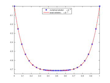
(a) $\varepsilon=2^{-3},\>N=32$

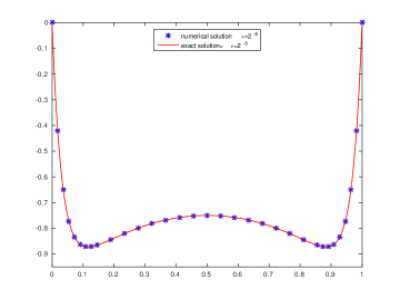
(b) $\varepsilon=2^{-5},\>N=32$

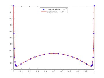
(c) $\varepsilon=2^{-7},\>N=32$

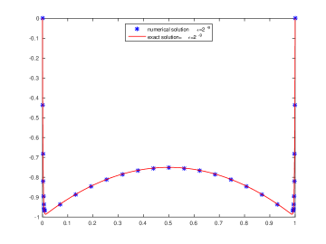
(d) $\varepsilon=2^{-9},\>N=32$

Figure 1: Graphics of the numerical and exact solutions for $N=32$ and $\varepsilon=2^{-3},\,2^{-5},\,2^{-7},\,2^{-9}$ for Example 6.1 and Example 6.3

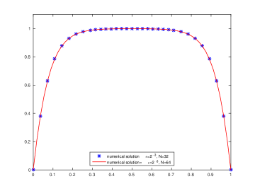
(a) $\varepsilon=2^{-3},\>N=32$

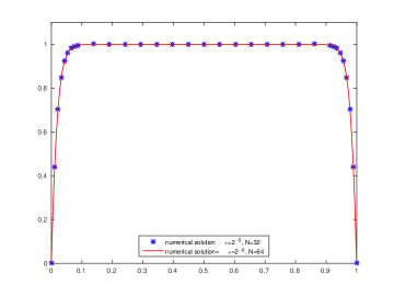
(b) $\varepsilon=2^{-5},\>N=32$

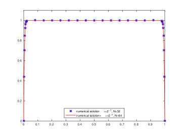
(c) $\varepsilon=2^{-7},\>N=32$

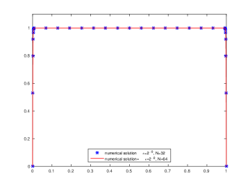
(d) $\varepsilon=2^{-9},\>N=32$

Figure 2: Graphics of the numerical and solutions for $N=32,\,64$ and $\varepsilon=2^{-3},\,2^{-5},\,2^{-7},\,2^{-9}$ for Example 6.2 and Example 63

Department of Mathematics
Faculty of sciences and Mathematics,
University of Tuzla
Univerzitetska 4, 75000 Tuzla,
Bosnia and Herzegovina
E-mail address: samir.karasuljic@untz.ba

Department of Mathematics
Faculty of sciences and Mathematics,
University of Tuzla
Univerzitetska 4, 75000 Tuzla,
Bosnia and Herzegovina
E-mail address: enes.duvnjakovic@untz.ba

Department of Mathematics
Faculty of sciences and Mathematics,
University of Tuzla
Univerzitetska 4, 75000 Tuzla,
Bosnia and Herzegovina
E-mail address: memic_91_elvir@hotmail.com

References

- [1] I. Boglaev, Approximate solution of a non-linear boundary value problem with a small parameter for the highest-order differential, Zh. Vychisl. Mat. i Mat. Fiz., 24(11), (1984), pp. 1649–1656.
- [2] E.P. Doolan, J.J.H. Miller and W.H.A. Schilders, Uniform numerical methods for problems with initial and boundary layers, Boole Press, Dublin, 1980.
- [3] E. Duvnjaković, S. Karasuljić and N. Okičić, Difference Scheme for Semilinear Reaction-Diffusion Problem, 14th International Research/Expert Conference Trends in the Development of Machinery and Associated Technology TMT 2010, 7. Mediterranean Cruise, (2010), pp. 793–796.
- [4] E. Duvnjaković and S. Karasuljić, Difference Scheme for Semilinear Reaction-Diffusion Problem on a Mesh of Bakhvalov Type, Mathematica Balkanica, 25(5), (2011), pp. 499–504.
- [5] E. Duvnjaković, S. Karasuljić, V. Pašić and H. Zarin, A uniformly convergent difference scheme on a modified Shishkin mesh for the singularly perturbed reaction-diffusion boundary value problem, Journal of Modern Methods in Numerical Mathematics 6(1), (2015), pp. 28-43.
- [6] E. Duvnjaković and S. Karasuljić, Uniformly Convergente Difference Scheme for Semilinear Reaction-Diffusion Problem, SEE Doctoral Year Evaluation Workshop, Skopje, Macedonia, 2011.
- [7] E. Duvnjaković and S. Karasuljić, Difference Scheme for Semilinear Reaction-Diffusion Problem, The Seventh Bosnian-Herzegovinian Mathematical Conference, Sarajevo, BiH, 2012.
- [8] E. Duvnjaković and S. Karasuljić, Class of Difference Scheme for Semilinear Reaction-Diffusion Problem on Shishkin Mesh, MASSEE International Congress on Mathematics - MICOM 2012, Sarajevo, Bosnia and Herzegovina, 2012.
- [9] E. Duvnjaković and S. Karasuljić, Collocation Spline Methods for Semilinear Reaction-Diffusion Problem on Shishkin Mesh, IECMSA-2013, Second International Eurasian Conference on Mathematical Sciences and Applications, Sarajevo, Bosnia and Herzegovina, 2013.
- [10] E. Duvnjaković, S. Karasuljić and N. Okičić, Difference Scheme for Semilinear Reaction-Diffusion Problem, 14th International Research/Expert Conference Trends in the Development of Machinery and Associated Technology TMT 2010, 7. Mediterranean Cruise, (2010), pp. 793–796.
- [11] E. Duvnjaković and S. Karasuljić, Uniformly Convergente Difference Scheme for Semilinear Reaction-Diffusion Problem, Conference on Appllied and Scietific Computing, Trogir, Croatia, pp. 25, 2011.
- [12] S. Karasuljić, E. Duvnjaković and H. Zarin, Uniformly convergent difference scheme for a semilinear reaction-diffusion problem, Advances in Mathematics: Scientific Journal 4(2), (2015), pp. 139–159.
- [13] S. Karasuljić, E. Duvnjaković, V. Pašić and E. Baraković, Construction of a global solution for the one dimensional singularly–perturbed boundary value problem, Journal of Modern Methods in Numerical Mathematics, 8(1–2), (2017), pp. 52–65.
- [14] S. Karasuljić and E. Duvnjaković, Construction of the Difference Scheme for Semilinear Reaction-Diffusion Problem on a Bakhvalov Type Mesh, The Ninth Bosnian-Herzegovinian Mathematical Conference, Sarajevo, BiH, 2015.
- [15] J. Lorenz, Stability and monotonicity properties of stiff quasilinear boundary problems, Zb.rad. Prir. Mat. Fak. Univ. Novom Sadu, Ser. Mat., 12, (1982), pp. 151–176.
- [16] G.I. Shishkin, Grid approximation of singularly perturbed parabolic equations with internal layers, Sov. J. Numer. Anal. M.Russian Journal of Numerical Analysis and Mathematical Modelling, 3(5), (1988), pp. 393–408.
- [17] G. Sun and M. Stynes, A uniformly convergent method for a singularly perturbed semilinear reaction-diffusion problem with multiple solutions, Math. Comput., 215(65), (1996), pp. 1085–1109.
- [18] Z. Uzelac and K. Surla, A uniformly accurate collocation method for a singularly perturbed problem, Novi Sad J. Math., 33(1), (2003), pp. 133–143.
- [19] R. Vulanović, On a Numerical Solution of a Type of Singularly Perturbed Boundary Value Problem by Using a Special Discretization Mesh, Novi Sad J. Math., 13, (1983), pp. 187–201.