Line-shape and Poles of the
Abstract
We study the non-Breit-Wigner line-shape of the resonance, predominantly a state, using an unitarized effective Lagrangian approach, including the one-loop effects of the nearby thresholds and . A fit of the theoretical result to the total cross-section is performed, leading to a good description of data (). The partial cross sections and turn out to be separately in good agreement with the experiment. We find a pole at MeV, that is within the Particle Data Group (PDG) mass and width estimation for this state. Quite remarkably, we find an additional, dynamically generated, companion pole at MeV, which is responsible for the deformation on the lower energy side of the line-shape. The width for the leptonic decay is 112 eV, hence smaller than the PDG fit of eV, yet in agreement with a recent experimental study.
keywords:
effective models, vector charmonia, poles, dynamical generation1 Introduction
The resonance is a vector state that was first detected at SPEAR [1] in 1977. The signal was fitted with a pure -wave Breit-Wigner distribution. More recently, the interest on this state was revived, and the parameters are nowadays fitted by the Particle Data group (PDG) as MeV for the mass and MeV for the width [2]. According to the ‘quark model review’ of the PDG, the resonance is classified as a charmonium state [3], the first one above the threshold, which is the reason for its relatively large width. As a consequence, besides kinematic interference, additional nonperturbative effects are expected.
Indeed, the line-shape of the resonance turned out to be quite anomalous. Although other experiments have been performed with observations in channel [4, 5, 6, 7, 8], the deformation on the line-shape of the was made clear by the BES Collaboration data in the annihilation to hadrons [9]. The existence of a second resonance was suggested, although possible dynamical effects, generated by the threshold were not discarded. A deformation of a line-shape due to the superposition of two resonances has been discussed before e.g., for the scalar kaon [10], where, besides the dominant state, an additional dynamically generated state arises from the continuum, the well known . Such effect has not been discussed before for the vector charmonium.
Various analysis of the have been performed. In Refs. [11, 12] fits were computed taking into account not only the interference but also the tail of the . Such inclusion is natural since the should be a mixed state -. In Ref. [13], the deformation from the right side of the resonance, i.e. a dip structure, is explained by the interference with the kinematical background which is higher for larger relative momentum. The same dip is reproduced in [11], using background only, in [14], where in addition, the continuum of light hadrons is removed, and in Refs. [15] and [16], using Fano resonances. In [17] BES measured an unexpectedly large branching fraction non of about , a result that is not contradicted by CLEO in [18], within errors. Predictions for such non- continuum were made including the tails of and , and decays [19], other excited states [20], the channel [21], other hadronic decays and radiative decays [12], and final state interactions [22], which in any case do not sum up to the value of . Yet, since the phase space to is not excessively large, it is likely that the missing decays are simply the sum of all the many Okubo-Zweig-Iizuka (OZI)-suppressed hadronic decays, that have not been studied systematically in the theory. Estimations for the production via annihilation are made in [23, 24, 25], which may possibly be measured at the PANDA experiment [26]. Mass estimations for the have also been made on the lattice [27, 28]. For a review of the charmonium states, see Ref. [29].
In this work, we study the properties of the by analyzing its production through electron-positron annihilation, and subsequent decay into pairs (for a preliminary study, see Ref. [30]). Our starting point is a vector charmonium seed state, which gets dressed by “clouds” of and mesons. Our aim is to study the deformation seen on the left side of the resonance in Ref. [9] with mesonic loops combined with the nearby thresholds. To this end, we use an effective relativistic Lagrangian approach in which a single vector state is coupled to channels and , as well as to lepton pairs. The propagator of is calculated at the resummed one-loop level and fulfills unitarization requirements. Then, we perform a fit of the four parameters of our approach, i.e. the effective couplings of to and of to leptons, the mass of , and a cutoff responsible for the finite dimension of the meson, to the experimental cross-section of the reaction in Refs. [7] and [5], in the energy region up to 100 MeV above the threshold. We assume that the resonance dominates in this energy range. We obtain a very good description of the data, which in turn allows us to determine in a novel and independent way the mass, width, and branching ratios of the . Moreover, we study in detail, to our knowledge for the first time, the poles of this state. In fact, a pole was found in Ref. [16], using Fano resonances, at about MeV, though in lesser detail. Quite remarkably, we find two poles for this resonance, one which roughly corresponds to the peak of the resonance, the seed pole, and one additional dynamically generated pole, responsible for the enhancement left from the peak, which emerges due to the strong coupling between the seed state and the mesonic loops. This is a companion pole, similar to the one found in the kaonic system in Ref. [10].
As a consequence of the determined parameters, we also show that the cross sections and agree separately to data. Being the resonance not an ideal Breit-Wigner one, different definitions for the partial widths are compared to each other. As a verification of our theoretical approach, we artificially vary the intensity of the coupling in order to show its effect on the line-shape of the resonance. Smaller couplings lead to a narrower Breit-Wigner-like shape, while larger couplings to an even larger deformation, which eventually gives rise to two peaks, as in Ref. [31]. In addition, the trajectory of each pole is analyzed, confirming the effects on the line-shape.
The paper is organized as it follows. In Sec. 2 the model is introduced and various theoretical quantities, such as the resummed propagator, spectral function, cross-section, and computation of the poles, are presented. In Sec. 3 we show our results: first, we present a fit to data and examine its consequences, then we study the position and trajectory of the poles. In Sec. 4 conclusions are drawn. Some important technical details and comparative results are discussed in the Appendices.
2 An Effective Model
In this section, we present the Lagrangian of the model and evaluate the most relevant theoretical quantities, namely the resummed propagator and the spectral functions, needed to calculate the cross section for the processes and , via production of the , and with one-loops.
2.1 The strong Lagrangian and dispersion relations
We aim to write down a Lagrangian for the strong interaction between a single vectorial resonance and two pseudoscalar mesons. The bare resonance is identified with a bare quarkonium state, with predominant quantum numbers , but admixtures of other quantum numbers, most notably the are possible. In our model, however, neither the quarkonium structure nor the orbital angular momentum mixing are explicit, since we work with mesonic degrees of freedom in the basis of total angular momentum. The effective strong Lagrangian density, for the charmonium state , reads
| (1) |
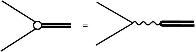
which corresponds to the simplest interaction among and its main decay products, the pseudoscalar pairs and , each vertex represented in Fig. 1. In this work, we shall take into account the small mass difference between and , i.e. isospin breaking for the masses, but we shall keep the same coupling constant, i.e. isospin symmetry for the decays, and we define . The full Lagrangian can be found in A.

|

|
|
|
|
|
The free propagator of a vector field , without any loops, with mass and momentum , is given by
| (2) |
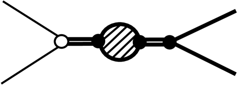
where the term in parenthesis is the sum over the three polarization states of a vector. We include the resummed one-loop effect as shown in Fig. 2, leading to the full propagator of
| (3) |
where is the loop-function, consisting of two contributions, the loops and the loops. In particular, we get
| (4) |
where the function , with , reads
| (5) |
where is the mass of the meson circulating in the loop (either or ), is the four-momentum of the loop, and (see B for computation details). Note, in the reference frame of the decaying particle, it holds the relation
| (6) |
An important element for our discussion is the vertex (or cutoff) function entering in Eq. (5). This is a form-factor that is needed to account for the unknown black vertices in Fig. 1, due to the fact that mesons are not elementary particles [32]. The cutoff function must ensure the convergence of the integral. We choose the following Gaussian form
| (7) |
where the second term is built up for convenience. In the isospin limit, reduces to . The parameter , introduced in Eq. (7), is on the same level of all the other parameters of our model and will be evaluated through our fit to data. Moreover, even if our form factor depends on the three-momentum only, hence strictly valid in the rest frame of the decaying particle, covariance can be recovered by properly generalizing the vertex function, see details in Ref. [33] 111One can formally introduce the vertex function already at the Lagrangian level by rendering it nonlocal, see the discussion in Refs. [34, 35, 36, 32], where it is also pointed out that the special form of the form factor is not important, as long as fast convergence is guaranteed.. However, the exponential form for the cutoff is very typical and has been used in many different approaches in hadron physics, e.g. Ref. [35]. For completeness, in C we shall also present the results for a different vertex function.
We now turn back to the study of the propagator. In B, it is shown that the relevant quantity is the transverse part of the propagator that, in the rest frame of the decaying particle, and for a single loop, reads
| (8) |
and similarly for the sum
| (9) |
The scalar part of the one-loop resummed dressed propagator reads
| (10) |
Note, this expression of the propagator fulfills unitarity (cf. Sec. 2.4 below) and it is accurate as long as further contributions to the self-energy are small 222 The next contribution would be represented by a loop in which the unstable state would be exchanged by mesons circulating in the loop. Such contributions are typically very small in hadron physics, as shown for instance in Ref. [37]. In addition, one could include also other channels, such as many other possible but suppressed decays of the (e.g., , etc…), as well as subthreshold channels such as that can contribute to the real part of the propagator..
The self-energy in Eq. (5) can either be computed through the integration (as in B), or using dispersion relations. We follow the latter. To this end, we first decompose into its real and imaginary parts
| (11) |
According to the optical theorem, the imaginary part (dispersive term) is given by
| (12) |
with being the center-of-mass momentum of the final mesons. The partial decay widths of and are then calculated as
| (13) |
| (14) |
where the Lorentz invariant amplitudes squared, computed from in Eq. (1), are given by
| (15) | |||
| (16) |
Note, by choosing the form factor as function of the energy [], when the imaginary part of the loop in Eq. (2.1) is taken, the replacement is performed (see Eqs. (15) and (16)). Then, the function directly enters in various expressions.
Finally, the on-shell partial and total decay widths are
| (17) | ||||
| (18) | ||||
| (19) |
Once the imaginary part of the loop is known, the real part, the function , is computed from the dispersion relation
| (20) |
where is zero below threshold. Convergence is guaranteed by the cutoff function. As we shall see in Sec. 3, the real part causes a distortion in the line-shape due to the continuous shifting of the physical mass of the resonance with the energy. Note, when the energy is complex, the function reads (away from the real axis):
| (21) |
This formula clearly shows that in the first Riemann Sheet (RS) the complex function is regular everywhere on the -complex plane, besides a cut from to infinity. In particular, in all directions 333In order to avoid misunderstanding, we recall that, in the 1st Riemann Sheet, the function is an utterly different complex function than . Namely, Eq. (21) implies solely that contains for being real. This fact is also clear by noticing that, while in any direction, diverges for .. Furthermore, although it is not strictly needed, since the integral in Eq. (20) is already convergent, we use the once-subtracted dispersion relation, with subtraction in point , for our convenience. Hence, the total loop-function is given by
| (22) |
and, the final dressed propagator of the meson is
| (23) |
In this way, the parameter in the propagator corresponds to the mass of the particle defined as
| (24) |
Other definitions for the mass are possible, such as the position of the peak, or the real part of the pole, as we shall see below.
2.2 Poles
In order to find poles, the energy is analytically continued to the complex plane (). In case of two decay channels, the Riemann surface is composed by four RSs. Poles are found in the unphysical sheet which results in the physical sheet when the energy is real and the resonance can be seen. Above both thresholds, this corresponds to the condition and when and , i.e., the third RS. Poles are given when the denominator of the propagator in Eq. (23) is zero in the correct RS, i.e.,
| (25) |
where
| (26) |
where the subscripts and stand for the first and third RS 444 In other terms, corresponds to see Eq. (6).. While in the first RS is regular everywhere apart from the cut(s) on the real axis (see Eq. (21) and subsequent discussion), in the other RSs the imaginary part continued to complex plane, appears. As a consequence, the vertex function generates a singular point at the complex infinity. When other choices for the vertex function are made, such as the one in C, other singularity types are generated. In general, any nontrivial function will display singularities appearing in RSs different from the first one.
2.3 Coupling to leptons
The available experimental data comes from the production process (see Fig. 4), therefore we need to couple the state to leptons. The corresponding interaction Lagrangian is defined by
| (27) |
which is the simplest interaction among a massive vector field and a fermion ()-antifermion pair. The coupling , between and the electron-positron pair, is here considered to be the same between and all leptonic pairs. It is the overall strength for the annihilation of the leptonic pair into one photon, and further conversion into the vector. In Eq. (27), we describe the process through a single effective vertex proportional to , but, as shown in Fig. 3, this coupling constant emerges via an intermediate virtual photon that converts into a charmonium state.
|
|---|
The corresponding decay into leptons reads
| (28) |
where is the leptonic mass. In principle, the loops of leptons should be included in the total one-loop function of resonance , obtaining , where dots refer to other possible but suppressed hadronic decay channels. However, the loop contribution of is definitely negligible w.r.t. Here, we shall simply consider
2.4 Spectral function and cross section
The unitarized spectral function as a function of energy , equivalent to the running mass of the resonance, is given by
| (29) |
that has the general shape of a relativistic Breit-Wigner distribution, distorted by the loop-function (cf. Eq. (22)). When no poles below threshold emerge, the normalization above threshold is guaranteed (unitarity):
| (30) |
The quantity is interpreted as the probability that the state has a mass between and The cross section for takes the form
| (31) |
Hence, the experimental data for this cross section give us direct access to the imaginary part of the propagator of the meson . The corresponding amplitude, leading to , is depicted in Fig. 4.
One also defines the partial spectral functions as [38]:
| (32) | |||
| (33) |
Then, the partial cross sections are given by:
| (34) | |||
| (35) | |||
| (36) |
3 Line-shapes and poles
In this section, we present our fit of Eq. (31) to experimental data and its consequences, and the notable existence, position, and trajectory of two poles underlying the .
3.1 Fit to data and consequences
As a first necessary step, we determine the four free parameters of our model
| (37) |
defined in Sec. 2, by performing a fit to the cross section data for the process . We use 14 experimental points published in Ref. [7], and the theoretical expression in Eq. (31). Note, we use only the data of Ref. [7] for the fit, since the data of Ref. [5] are contained in the data samples of Ref. [7] (the data sets of March 2001 quoted in these two papers are the same [39]). The fit to data is shown in Fig. 5, and the values of the parameters in the set (37) are presented in Table 1. We get the value , which shows that a very good description of the data is achieved.
The errors of the parameters entering the fit are estimated by the square root of the corresponding Hessian matrix (this is a result of the standard procedure according to in which one defines a new set of parameters that diagonalize the Hessian matrix, see e.g. Ref. [40] for details).
There are various consequences of the fit that we discuss in detail:

| (MeV) | |
|---|---|
| (MeV) | |

|

|
| (MeV) | ||
|---|---|---|
| (MeV) | ||
| (MeV) | ||
a) The value of the mass MeV (corresponding to the zero of the real part of the inverse’s propagator, see Eq. (24)) is in well agreement with the current PDG fit of MeV [2].
b) In Fig. 6 we present a comparison between theory and the data for the cross sections and , using the parameters in Table 1. The good agreement shows that the theory is able to describe the two partial cross sections separately, without the need of some extra parameter, and in agreement with isospin symmetry.
c) The branching ratios and partial and total () widths are presented in Table 2. The partial widths, evaluated on-shell, are defined in Eqs. (17)-(19). The branching ratios are in agreement with those quoted in PDG for the . The ratio of is compatible with the PDG values, which range from to . However, as shown in Fig. 7, the functions and strongly vary in the region of interest. Alternatively, one may use a different definition, cf. [32], to obtain the partial decay widths and the full decay width to , by integrating over the spectral function as
| (38) | |||
| (39) | |||
| (40) |

A somewhat naive but still useful alternative determination of the mass is the value corresponding to the peak and the half-height width:
| (41) |
where we estimated the error of the peak mass as MeV, close to the determined error for the parameter , and the error of the distribution width as MeV as well, coincident to the error for (see Table 2). These evaluations show that the resonance is far from being an ideal Breit-Wigner. While all these different approaches coincide for states with a very small width, here the distortions are sizable, hence clear definitions of mass and width, as well as branching ratios, are difficult. A commonly used approach to get a uniform result, makes use of poles in the complex plane, as we show in Sec. 3.2.
This discussion shows that there is no unique definition of the total and the partial widths. This fact also renders a direct comparison with the fit of the PDG quite difficult. Namely, according to PDG, one has MeV, MeV, and MeV [2], hence our results for the partial decay widths evaluated on shell and presented in Table 2, first column, are somewhat smaller. However, as visible in Fig. 7, the corresponding function vary strongly in the energy region of interest. Moreover, instead of using theoretical partial widths which cannot be uniquely defined, one should stress that our approach correctly describes the data for channels and separately, as visible in Fig. 6, and as described in point b) above.
Another commonly used approach to circumvent all these definition problems mentioned above, is to move away from the real axis and to study the pole(s) in the complex plane. As we shall see in detail in Sec. 3.2, the seed pole of corresponds to a larger decay width of MeV which is in very well agreement with PDG.
d) Using the coupling that outcomes from the fit, the widths can be easily computed from Eq. (28). Results are shown in Table 3. The value for is smaller than the one given by the PDG fit of eV by a factor two, but it is compatible with the analysis in Ref. [8], that gives eV. The mismatch of our result with the PDG estimate, that nevertheless lists a quite broad range of values from different experiments, shows that this decay rate should be further investigated in the future. Also the experimental identification of the decays into and could help to distinguish among different models.
| (eV) | (eV) | (eV) |
|---|---|---|
e) The Gaussian vertex function together with the cutoff value MeV takes into account in a simple way the composite nature of the resonance and its nonlocal interaction with the mesons. Microscopically the vertex function emerges from the nonlocal nature of both and of the decay products (for point-like part interaction, goes to infinity), see Refs. [35, 26] for an explicit treatment. (Indeed, the rather small value of emerging from our fit is intuitively understandable by the fact that the resonance is predominantly a wave. A detailed study of this issue by using a microscopic model such as the one in Ref. [41] will be given elsewhere). The vertex function is a crucial ingredient that defines our model and, among other properties, guarantees the finiteness of the results. The exponential form used here emerges naturally from various microscopic approaches, see Refs. [41, 42] and refs. therein. However, our results do not strongly depend on the precise choice of the vertex function as long as it is smooth and at the same time falls sufficiently fast. As we show in C, a hard cutoff would imply that the spectral function would fall abruptly to zero above a certain threshold; this unphysical behavior does not lead to any satisfactory description of data. On the other hand, as discussed in D, the avoidance of a form factor through a three-times subtracted dispersion relation does not lead to satisfactory results, thus confirming that the need of some vertex function for our treatment of mesonic loops is needed. Once the vertex function is fixed, the model is mathematically consistent at any energy: in fact, the important normalization condition reported in Eq. (30) is obtained by formally integrating up to infinity (numerically, the normalization is verified by integrating up to GeV). In turn, this means that, from a mathematical perspective, the value of the momentum of the emitted mesons can be larger than A different issue is the maximal energy up to which we shall trust our model. In fact, even if mathematically consistent, the model is limited because it takes into account only one vector resonance and neglects the contributions of other resonances, most notably as well as the background (see the comments h) and i) about these topics) and the next opening thresholds, such as . We therefore trust the model in the energy range starting from the lowest threshold, , up to at most GeV, when the line-shape goes down and, as described in Refs. [11, 12], the role of the background becomes important.
f) In our fit, we consider only the resonance as a virtual state of the process . As discussed above, a possible mixing between bare states with quantum numbers and is automatically taken into account in our bare field entering into the Lagrangian defined in Eq. (1). Indeed, the bare field, i.e., the field prior to the dressing by mesonic loops, represents the diagonal quark-antiquark state, while the is a mixture of and configurations, with the as its orthogonal state. Yet, the role of the as an additional exchange in the reaction was not taken into account. Being off-shell in the energy of interest, the propagator is expected to suppress this amplitude; moreover, also its coupling to channel is expected to be small, due to the form-factor. Indeed, in Refs. [43, 44], the , loops, and rescattering have been considered, leading to fits that are in good agreement with the experiment in Ref. [7]. In both references the contribution is quite small, in agreement with our results. However in their case the was still necessary to obtain a good fit, whereas in our model it is not. Note, in Refs. [43, 44] the pole structure was not examined.
g) In this work we did not consider a four-leg interaction process of the type that can be formally described by a four-vertex proportional to . Such a rescattering describes elastic scattering, induced by a direct four-body interaction, and also as an effective description of various -channel exchanges between . Our model can describe properly the data without this contribution, hence the inclusion of a four-leg interaction is not needed to improve the agreement with the data. This does not necessarily mean that its magnitude is small, but simply that one can hardly disentangle its role from the -loops that we have considered in our approach. In addition, there is a more formal point that should be taken into account: one can in principle redefine the field where is a parameter on which no physical quantity should depend on [45, 46]. The redefinition would however lead to some rescattering terms. Of course, the independence on the field redefinition can be fully accomplished only if one could solve the theory exactly, since in any approximation scheme differences would still persist at a given order. In conclusion, the study of a four-leg interaction term (as well as other effects such as the mixing with ) should be performed when more precise data will be available.
h) Here, we discuss more closely the differences between our work and the one in Ref. [43]. The main difference is the treatment of the propagator of the meson, in particular for what concerns the self-energy. In Ref. [43] the imaginary part of the self-energy (i.e., the energy-dependent decay width) grows indefinitely with increasing In this way, the Källén–Lehmann representation does not lead to a normalized spectral function. Moreover, the real part of the self-energy depends on an additional subtraction constant (linked to the regularization of the loop in Ref. [43], hence ultimately corresponding to our cutoff ). When is set to zero (their so-called minimal subtraction scheme) the real part of the self energy simply vanishes (hence, it is trivial). When is different from zero, the real part also grows indefinitely for increasing Indeed, in the approach of Ref. [43], the propagator of is not enough to describe data, also when the rescattering is present; the inclusion of the state is necessary. Hence, our approach is different under many aspects: since it contains a fully consistent treatment of loops, the dispersion relations are fulfilled and the normalization of the spectral function is naturally obtained. In this way, nontrivial effects which modify the form of the spectral function automatically arise. Moreover, in our case neither the nor the rescattering are needed to describe the data, hence the physical picture of the two models is rather different. In conclusion, the fit in Ref. [43] is performed with six parameters (repeated for different values of the subtraction constant , for a total of seven), while we use only 4. Both approaches can describe data: in the future, better data are needed to understand which effects are more important. Our work suggests that the nearby threshold and loops are necessary to correctly understand the . Furthermore, the presence of two poles is a stable prediction of our approach, see Secs. 3.2 and 3.3 below.
i) As a last comment, we compare our result with the approach of Refs. [11, 12]. Interestingly, in Ref. [12] it is shown that a suppression of the cross-section at about GeV is obtained by a destructive interference of the resonance with the background. This outcome is useful, since it sets a physical limit for our approach, in which no background is present: our description of data cannot be expected above this upper limit (and indeed we perform the fit below it). However, for what concerns the treatment of our model is quite different: in Refs. [11, 12] rescattering is taken into account. When their rescattering parameter is set to zero, the real part of the loop vanishes. In contrast, in our approach, even without an explicit rescattering term, the loops are taken into account in a way that guarantees the unitarity expressed by Eq. (30) (its fulfillment is one of the most relevant technical aspects of our approach) and they are found to be important for a proper description of the .
3.2 Pole positions
As renowned, a theoretically (and lately experimentally as well, see e.g. the in PDG) stable approach to describe unstable states is based on the determination of the position of the corresponding poles. In the present case, one obtains, quite remarkably, two poles on the III Riemann Sheet. As seen in Sec. 2.2, this is the sheet relevant for a system with two decay channels at energy above both thresholds. In the isospin limit, the III RS reduces to the usual II RS. In the following, the indeterminacy of the pole masses is estimated to be MeV, close to the error obtained for the parameter , and the indeterminacy of the pole width(s) as MeV, coincident with the error for (see Table 2). In fact, the errors of these strictly correlated quantities must have a similar magnitude. The closest pole to the Riemann axis reads:
| (42) |
hence
| (43) |
which agrees quite well with the PDG values [2]. This pole is closely related to the seed charmonium state and to the position and width of the peak. Furthermore, a second broader pole appears at lower energy:
| (44) |
This pole is dynamically generated, and it is related to the the deformation of the signal on the left side. It is also referred to as a companion pole emergent due to the strong dynamics. The situation is very much reminiscent of the light scalar state at lower energy, which was interpreted as a dynamically generated companion pole of in Refs. [10, 33]. For additional recent works on this state, see Refs. [47, 48], and references therein. This similarity is interesting also in view of an important difference between the two systems: the decay of a scalar kaon into two pseudoscalars is a -wave () while that of a vector charmonium into two pseudoscalars is a -wave ().
We mention again C, where a different form factor is used. The results turn out to be very similar and also in that case two poles, very close to the ones discussed here, are found.
No other poles could be numerically found in the complex plane. As discussed in comment e), the energy scale does not represent a limit of validly of our approach. Yet, since the numerical value of MeV preferred by the fit is rather small (the value of the emitted momentum is comparable to it), it is interesting to investigate if two poles exist also when artificially increasing its value. Upon fixing MeV, one gets hence the description of data is worsened () but still qualitatively acceptable; nevertheless, there are still two poles: the seed one corresponds to GeV (somewhat too large) and the broad dynamically generated one to GeV. Upon increasing even further to MeV, the worsens, i.e. (which is already beyond the border of a satisfactory description of data), but there are still two poles; the seed pole reads GeV and the companion pole GeV. This exercise shows that the presence of two poles is a stable result also when changing the value of , even to values which are safely larger than the value of the modulus of the outgoing momentum of the meson (even if the data description gets worse for increasing ).
3.3 Pole Trajectories
Here we study the effect of varying the coupling constant over the line-shape and over the pole positions. We define as the variable parameter (upon varying the scaling factor ) and let be fixed to the value in Table 1. In Quantum Chromodynamics (QCD), a change in such coupling is equivalent to vary the number of colors according to the scaling . Results are shown in Fig. 8 for the cross-section, and in Table 4 for pole positions. The pole trajectories, as a function of , are depicted in Fig. 9. As expected, as decreases, the cross section approaches a Breit-Wigner-like shape, see case where in Fig. 8. Figure 9 shows that, as gets smaller, the first pole, from the seed, gets closer to the real axis, while the second pole, dynamically generated, moves deeper in the complex plane until it disappears at the threshold for a certain critical value, in this case (corresponding to ). On the contrary, when increases, the first pole runs away from the real axis, while the second pole approaches it. Eventually, the dynamically generated pole gets even closer to the real axis than the seed pole, as it is shown for the case where . For such a value of (or larger), the second pole originates a second peak in the line-shape (see Fig. 8).

| Pole 1 | |||
|---|---|---|---|
| Pole 2 |

4 Summary, Conclusions, and Perspectives
Vector mesons can be produced by a single virtual photon, hence they play a crucial role in the experimental study of QCD. The renowned charmonium vector state opened a new era in hadron physics and it is one of the best studied resonances (cf. [2]). Here, we have focused on an orbital excitation of the , the meson , whose mass lies just above the threshold. For this reason, this resonance is extremely interesting. The cross-section encloses nonperturbative phenomena nearby the OZI-allowed open decay channel . The production and decay to all hadrons shows evidence of a deformation on the line-shape of the resonance [9].
In this work, we presented an unitarized effective Lagrangian model, with one bare orbital seed state dressed by mesonic loops, that has never been employed before to this system. In particular, our model accounts for one-loop contributions by fulfilling unitarity of the spectral function. Using four parameters only, we obtain a satisfactory fit to the cross-section data ( ). Moreover, the theoretical cross section is in good agreement with data in channels and separately. Partial widths are also in agreement with the PDG values. The partial decay to leptons is smaller than the average in PDG, but still reasonable (and in agreement with Ref. [8]). The cutoff parameter , inversely proportional to the size of the wave-function, turns out to be rather small, possibly due to the fact that the is a -wave. Other effects, such as final state rescattering modelled by a four-leg interaction term, or the contribution of the tail of the to the amplitude, are not taken into account, since our fit is already very good without them (this represents a difference with Ref. [43], where these terms were necessary to describe data but where the normalization of the spectral function of was not guaranteed). The detailed study of the role of these additional effects within our framework needs more precise data and is left for the future.
An important result of our work is the evaluation of two poles at and , the first is a standard seed pole, very close to the one determined by BES in Ref. [9], and the second broader pole is dynamically generated, being an additional companion pole. The presence of a second pole explains the deviation from a pure Breit-Wigner line-shape. By varying the coupling constant , we studied the pole trajectories and its influence over the line-shape. For small couplings the dynamical pole disappears and the seed pole approaches the real axis, leading to a Breit-Wigner-like line-shape, while for larger couplings the dynamical pole approaches the real axis while the seed pole moves down and to the right, and a second peak becomes evident (see Figs. 8 and 9 for details). The width of about 24 MeV to channel , that we obtain from the first pole, is consistent with the experimental measurements to this channel, and with the branching fraction estimated to be about in Ref. [49], considering that measurements of the width in decays to all hadrons are a few MeV higher (cf. Ref. [2]).
A natural outlook is the inclusion of the many OZI-suppressed hadronic decay channels. A related topic is the evaluation of mixing with the vector glueball, whose mass is predicted to be at about 3.8 GeV by lattice QCD [50]. Finally, the same theoretical approach used in this work can be applied to other resonances whose nature is not yet clarified, the so-called and states [51, 52, 53]. It is well possible that some of these resonances arise as companion poles due to a strong coupling of a standard charmonium seed state to lighter mesonic resonances. The strong dressing of the original state with meson-meson clouds generates new poles and new peaks. An intriguing possibility is that the additional peak arises at a higher energy than the seed state, see Refs. [54, 55, 56, 57] for a phenomenological description of this phenomenon in the light sector. Hence, detailed studies of the dynamics underlying each line-shape, that consider poles and interference with the main hadronic degrees of freedom, may shed light on some newly discovered resonances in the charmonium region.
An interesting outlook should be the description of the whole sector above the threshold. To this end, one should develop a unique treatment of the four standard charm-anticharm resonances above the threshold , , , and (and also the resonance below). In this way, following and extending the discussion in Refs. [41, 43], all quantum mixing terms should be properly taken into account. The aim of such an ambitious project would be the simultaneous description of the whole sector as well as the description of (some of the) newly observed resonances in this energy region, which might emerge as dynamically generated states.
Acknowledgements
We thank G. Rupp and E. van Beveren for useful discussions. This work was supported by the Polish National Science Center through the project OPUS no. 2015/17/B/ST2/01625.
Appendix A Full Lagrangian
The complete form of the Lagrangian used in this work is given by:
Appendix B Details of the Loop Function
Here, we derive the propagator of the vector resonance dressed by loops. The considerations are however general, and they can be applied to loops of each vector state. Using the shortening notations
| (48) | |||
| (49) |
we decompose the tensor loop contribution in its transverse and longitudinal parts (see e.g. Ref. [58]):
Then, multiplying by and , respectively, we get:
| (50) | |||
| (51) |
out of which we find, in the rest-frame of the decaying particle, , where is the running mass of the :
| (52) | ||||
| (53) | ||||
| (54) |
Namely, its imaginary part implies that is replaced by and by . Explicitly, it reads:
| (55) |
as it should. Similarly, for the sum of the two contributions, one has:
| (56) | |||
| (57) |
Indeed, an explicit resummation of the full propagator shows that
| (58) |
where we have used
| (59) |
The final result reads
| (60) |
where it is evident that the first part contains the properties of the unstable state.
Appendix C Using a different Cutoff Function
The use of an exponential vertex function is a typical choice in hadron physics. (It is also used as a form factor in various phenomenological approaches [3, 42]. Yet, for completeness, we test here a different cutoff function, chosen as:
| (61) |
where being the mass of the particle circulating in the loop. In the isospin limit the vertex function reduces to Since in the loop integral the squared function enters, convergence is guaranteed (see also Eqs. (52)-(55)). Notice that a simple dipole function of the type would not fall fast enough.
Clearly, also with Eq. (61) the loop function expressed in Eq. (21) is, besides a cut on the real axis, regular everywhere in the first Riemann sheet. In the second Riemann sheet of , it enters the vertex function , continued to the complex plane, and additional poles emerge.
Let us now present the results. By performing the very same fit as in Sec. 3, we find a minimum for , which is even smaller than the one reported in Table 1. The corresponding cutoff MeV, mass , and coupling to leptons are very similar to those in Table 1. Only the coupling constant turns out to be slightly smaller, . However, the tree-level decay widths MeV and MeV are basically unchanged. Also the spectral function and the cross-sections have a very similar form, hardly distinguishable to the ones presented in Sec. 3.
Finally, we turn to the poles. Also in this case two poles are found, the first at MeV, very similar to Eq. (42), and the second at MeV, which corresponds well to Eq. (44). The presence of two poles is stable against parameter variations, in a way very much similar to Fig. 9.
This exercise shows that the precise form of the vertex function does not affect the results as long as it falls off sufficiently fast. On the other hand, the numerical value of the cutoff energy scale is crucial.
Appendix D Three-time subtracted dispersion relation
As seen in the main text through the Gaussian vertex function, and in the previous Appendix through a dipole-like function, an energy scale of about - MeV emerges from fits to data. Yet, it is interesting to test a completely different strategy: a three-time subtracted dispersion relation, in which no energy scale appears (namely, one needs to subtract at least three times to guarantee convergence, see below). The explicit form of the scalar part of the propagator of the meson reads:
| (62) | |||||
where and are a convenient rewriting of the three subtraction constants. Moreover,
| (63) |
are the tree-level decay widths obtained from the Lagrangian of Eq. (1) (without any form factor, hence valid in the local limit), and the real parts read
| (64) | |||||
| (65) |
(for below threshold the integrals are real and the principal part is omitted). These integrals are convergent in due to the factor in the denominator of the integrand.
The constant is easily obtained as in such a way that is the zero of . The constant can be used to guarantee the normalization of the spectral function.
We then performed a fit to data involving the following four parameters: , , , and . Roughly speaking, the constant replaces the cutoff . The results for this set-up are not satisfactory. One obtains various local minima for the of the order of (hence, , which in practice means that no reasonable description of data is obtained).
Notice that the three-time subtracted dispersion relation is not equivalent, within our treatment, to a hard cutoff. Namely, such a hard cutoff would imply that the spectral function is proportional to In this way the normalization condition of Eq. (30) would still be fulfilled (at the price of having a rather unphysical behavior of the spectral function, which goes abruptly to zero above a certain energy threshold). However, such a procedure is clearly different from the here presented dispersion relation, in which the imaginary part of the propagator is nonzero for any value of above the threshold. An equivalence of the treatments can be achieved only when considering the cutoff as a very large number: but, as we explained in the text, we regard the cutoff function as a physical quantity describing the finite dimension of mesons and their interactions (in fact, a similar cutoff function emerges in the context of the microscopic model) and we do not consider the limit
Moreover, even if a hard cutoff is not physical for the treatment of the , it was used in various studies and is also capable to generate additional poles, as long as its value is finite and of the same order of (or not much larger than) the energy scale of the system (see Ref. [32] and Refs. therein). In fact, when is finite, the real part is not a simple constant and additional nontrivial features of the propagator appear.
In conclusion, the negative result of the three-time subtracted dispersion relation is nevertheless instructive, since it shows that a form factor which takes into account the finite dimensions of mesons and of their interactions seems to represent a rather physical feature needed for a correct description of loops.
References
- [1] P.A. Rapidis et al., Observation of a Resonance in Annihilation Just above Charm Threshold, Phys. Rev. Lett. 39, 526 (1977).
- [2] M. Tanabashi et al. (Particle Data Group), Phys. Rev. D. 98, 030001 (2018).
- [3] S. Godfrey and N. Isgur, Mesons in a relativized quark model with chromodynamics, Phys. Rev. D. 32, 189 (1985).
- [4] R. Christov et al. (Belle Collaboration), Observation of , Phys. Rev. Lett. 93, 051803 (2004).
- [5] M. Ablikim, et al. (BES Collaboration), Measurements of the Branching Fractions for , and the Resonance Parameters of and , Phys. Rev. Lett. 97, 121801 (2006).
- [6] B. Aubert, et al. (BABAR Collaboration), Study of the exclusive initial-state-radiation production of the system, Phys. Rev. D 76, 111105 (R) (2007).
- [7] M. Ablikim, et al. (BES Collaboration), Measurements of the line-shapes of production and the ratio of production rates of and in annihilation at , Phys. Lett. B 668, 263 (2008).
- [8] V.V. Anashin et al., Measurement of parameters, Phys. Lett. B 711, 292 (2012).
- [9] M. Ablikim, et al. (BES Collaboration), Anomalous Line Shape of the Cross Section for Hadrons in the Center-of-Mass Energy Region between 3.650 and 3.872 GeV, Phys. Rev. Lett. 101, 102004 (2008).
- [10] T. Wolkanowski, M. Sołtysiak, and F. Giacosa, as a companion pole of , Nuc. Phys. B 909, 418 (2016).
- [11] N.N. Achasov and G.N. Shestakov, Line shape of in , Phys. Rev. D 86, 114013 (2012).
- [12] N.N. Achasov and G.N. Shestakov, Description of the resonance interfering with the background, Phys. Rev. D 87, 057502 (2013).
- [13] E. van Beveren and G. Rupp, Production of hadron pairs in annihilation near the , , , and thresholds, Phys. Rev. D 80, 074001 (2009).
- [14] R. Wang, X. Cao, and X.R. Chen, The value in the vicinity of state, Phys. Lett. B 747, 321 (2015).
- [15] X. Cao and H. Lenske, Charmonium resonances and Fano line shapes, arXiv:1408.5600 [hep-ph].
- [16] X. Cao and H. Lenske, The nature and line shapes of charmonium in the reactions, arXiv:1410.1375 [hep-ph].
- [17] M. Ablikim et al. (BES Collab.), Measurements of the cross sections for at 3.650, 3.6648, 3.773 GeV and the branching fraction for , Phys. Lett. B 641, 145 (2006).
- [18] D. Besson et al. (CLEO Collaboration), Measurement of at MeV, Phys. Rev. Lett. 96, 092002 (2006).
- [19] A.G. Shamov and K.Yu. Todyshev, Analysis of BaBar, Belle, BES-II, CLEO and KEDR data on line shape and determination of the resonance parameters, Phys. Lett. B 769, 187 (2017).
- [20] H.B. Li, X.S. Qin, and M.Z. Yang, Study of the branching ratio of in scattering, Phys. Rev. D 81, 011501(R) (2010).
- [21] G. Li, X.H. Liu, Q. Wang, and Q. Zhao, Further understanding of the non- decays of , Phys. Rev. D 88, 014010 (2013).
- [22] X. Liu, B. Zhang, and X.Q. Li, The puzzle of excessive non- component of the inclusive decay and the long-distant contribution, Phys. Lett. B 675, 441 (2009).
- [23] M. Ablikim et al., Study of in the vicinity of the , Phys. Rev. D 90, 032007 (2014).
- [24] H. Xu, J.J. Xie, and X. Liu, Implications of the observed for studying , Eur. Phys. J. C 76, 192 (2016).
- [25] J. Haidenbauer and G. Krein, resonance and its production in , Phys. Rev. D 91, 114022 (2015).
- [26] M. F. M. Lutz et al. [PANDA Collaboration], Physics Performance Report for PANDA: Strong Interaction Studies with Antiprotons, arXiv:0903.3905 [hep-ex].
- [27] C.B. Lang, L. Leskovec, D. Mohler, and S. Prelovsek, Vector and scalar charmonium resonances with lattice QCD, JHEP 09, 089 (2015).
- [28] J.J. Dudek, Charmonium excited state spectrum in lattice QCD, Phys. Rev. D 77, 034501 (2008)
- [29] D. Bettoni, R. Calabrese, Charmonium spectroscopy, Prog. Part. Nuc. Phys. 54, 615 (2005).
- [30] S. Coito and F. Giacosa, Formation and Deformation of the , Acta Phys. Pol. B Proc. Supp. 10, 1049(2017).
- [31] T. Wolkanowski, F. Giacosa and D. H. Rischke, revisited, Phys. Rev. D 93, 014002 (2016).
- [32] F. Giacosa and G. Pagliara, Spectral functions of scalar mesons, Phys. Rev. C 76, 065204 (2007).
- [33] M. Soltysiak and F. Giacosa, A covariant nonlocal Lagrangian for the description of the scalar kaonic sector, Acta Phys. Polon. Supp. 9, 467 (2016).
- [34] R. D. Bowler and M. C. Birse, A Nonlocal, covariant generalization of the NJL model, Nucl. Phys. A 582, 655 (1995)
- [35] A. Faessler, T. Gutsche, M. A. Ivanov, V. E. Lyubovitskij and P. Wang, Pion and sigma meson properties in a relativistic quark model, Phys. Rev. D 68, 014011 (2003).
- [36] F. Giacosa, T. Gutsche and A. Faessler, A Covariant constituent quark gluon model for the glueball-quarkonia content of scalar - isoscalar mesons, Phys. Rev. C 71, 025202 (2005)
- [37] J. Schneitzer, T. Wolkanowski and F. Giacosa, The role of the next-to-leading order triangle-shaped diagram in two-body hadronic decays, Nucl. Phys. B 888, 287 (2014)
- [38] F. Giacosa, Non-exponential decay in quantum field theory and in quantum mechanics: the case of two (or more) decay channels, Found. Phys. 42, 1262 (2012).
- [39] Private communication with Guang Rong, from BES Collaboration.
- [40] M. Piotrowska, C. Reisinger and F. Giacosa, Strong and radiative decays of excited vector mesons and predictions for a new resonance, Phys. Rev. D 96, 054033 (2017).
- [41] S. Coito, Radially excited axial mesons and the enigmatic and in a coupled-channel model, Phys. Rev. D 94, 014016 (2016).
- [42] C. Amsler and F.E. Close, Is a scalar glueball?, Phys. Rev. D 53, 295 (1996).
- [43] G.Y. Chen and Q. Zhao, Study of the anomalous cross-section lineshape of at with an effective field theory, Phys. Lett. B 718, 1369 (2013).
- [44] Y.J. Zhang, and Q. Zhao, Lineshape of and low-lying vector charmonium resonance parameters in , Phys. Rev. D 81, 034011 (2010).
- [45] S. Weinberg, Elementary Particle Theory of Composite Particles, Phys. Rev. 130, 776 (1963); Quasiparticles and the Born Series Phys. Rev. 131, 440 (1963); Evidence That the Deuteron Is Not an Elementary Particle Phys. Rev. 137, B672 (1965).
- [46] V. Baru, C. Hanhart, Yu.S. Kalashnikova, A.E. Kudryavtsev, and A.V. Nefediev, Interplay of quark and meson degrees of freedom in a near-threshold resonance, Eur. Phys. J. A 44, 93 (2010).
- [47] J. R. Pelaez and A. Rodas, The non-ordinary Regge behavior of the or -meson versus the ordinary , Eur. Phys. J. C 77, 431 (2017).
- [48] J. R. Pelaez and A. Rodas, Pion-kaon scattering amplitude constrained with forward dispersion relations up to 1.6 GeV, Phys. Rev. D 93, 074025 (2016).
- [49] M. Ablikim et al. (BES Collaboration), Direct measurements of the cross sections for hadrons in the range from 3.65 to 3.87 GeV and the branching fraction for , Phys. Lett. B 659, 74 (2008).
- [50] Y. Chen et al., Glueball spectrum and matrix elements on anisotropic lattices, Phys. Rev. D 73, 014516 (2006).
- [51] H. X. Chen, W. Chen, X. Liu and S. L. Zhu, The hidden-charm pentaquark and tetraquark states, Phys. Rept. 639, 1 (2016).
- [52] A. Esposito, A. Pilloni, and A.D. Polosa, Multiquark resonances, Phys. Rep. 668, 1 (2017).
- [53] D. Gamermann and E. Oset, Hidden charm dynamically generated resonances and the reactions, Eur. Phys. J. A 36, 189 (2008).
- [54] E. van Beveren, T. A. Rijken, K. Metzger, C. Dullemond, G. Rupp, and J. E. Ribeiro, A Low Lying Scalar Meson Nonet in a Unitarized Meson Model, Z. Phys. C 30, 615 (1986).
- [55] M. Boglione and M. R. Pennington, Dynamical generation of scalar mesons, Phys. Rev. D 65, 114010 (2002).
- [56] N. A. Tornqvist, Understanding the scalar meson q anti-q nonet, Z. Phys. C 68, 647 (1995).
- [57] V. R. Debastiani, F. Aceti, W. H. Liang and E. Oset, Revising the resonance, Phys. Rev. D 95, 034015 (2017).
- [58] H. B. O’Connell, B. C. Pearce, A. W. Thomas and A. G. Williams, mixing, vector meson dominance and the pion form-factor, Prog. Part. Nucl. Phys. 39, 201 (1997).