Hillclimbing saddle point inflation

Abstract

Recently a new inflationary scenario was proposed in Jinno:2017jxc which can be applicable to an inflaton having multiple vacua. In this letter, we consider a more general situation where the inflaton potential has a (UV) saddle point around the Planck scale. This class of models can be regarded as a natural generalization of the hillclimbing Higgs inflation Jinno:2017lun .

The Standard Model (SM) of particle physics is the most successful theory that describes physics below the TeV scale. The observed Higgs mass $\sim 125$GeV indicates that the SM can be safely interpolated up to the Planck scale without any divergence or instability. Furthermore, the observed Higgs quartic coupling $\lambda\sim 0.12$ also shows an interesting behavior of the Higgs potential around the Planck scale $M_{pl}$; The potential can have another degenerate minimum around that scale. The origin of this behavior comes from the fact that $\lambda$ and its beta function $\beta_{\lambda}$ can simultaneously vanish around $M_{pl}$. This is called the Multiple point criticality principle and it is surprising that the Higgs mass was predicted to be around $130$GeV about 20 years ago based on this principle Froggatt:1995rt .
Various phenomenological and theoretical studies of such a degenerate vacuum have been done so far Holthausen:2011aa ; Bezrukov:2012sa ; Degrassi:2012ry ; Nielsen:2012pu ; Buttazzo:2013uya . One of them is the Higgs inflation with a non minimal coupling $\xi\phi^{2}R/M_{pl}^{2}$ Bezrukov:2007ep . When this scenario was proposed, it was argued that we need large $\xi\sim 10^{5}$ in order to obtain the successful inflationary predictions of the cosmic microwave background (CMB). However, the criticality of the Higgs potential makes it possible to realize the inflation even if $\xi$ is relatively small $\sim{\cal{O}}(10)$ by using small but nonzero $\lambda\sim 10^{-6}$ around $M_{pl}$. See Hamada:2014wna for the detailed analyses.
Although the SM criticality can help the realization of the Higgs inflation, it is difficult to realize the MPP simultaneously because the latter requires $\lambda=0$ around the Planck scale and we can no longer maintain the monotonicity of the Higgs potential above the scale $\sim M_{pl}/\sqrt{\xi}$. Recently, a new inflationary scenario was proposed in Jinno:2017jxc which enables an inflation even if the inflaton potential has multiple degenerate vacua. Then, the authors applied it to the SM Higgs and showed that it is actually possible to obtain a successful inflation while satisfying the MPP Jinno:2017lun . In those papers, the authors studied a few cases such that the inflaton potential behaves as a quadratic potential around another potential minimum. Although the inflationary predictions of this scenario does not strongly depend on the details of the inflaton potential such as the coefficients of the Taylor expansion, they can depend on the leading exponent of the (Jordan-frame) potential and the choice of the conformal factor. In this letter, we generalize their works to the cases where the inflaton potential has a saddle point around the Planck scale. Our study is meaningful from the point of view of the MPP because this situation can be understood as a natural generalization of this principle. Although some fine-tunings are needed in order to realize a saddle point, some theoretical studies Hamada:2014ofa ; Hamada:2014xra ; Hamada:2015dja ; Kawana:2016tkw suggest that we can naturally archive such fine-tunings by considering physics beyond ordinary field theory.

I Brief Review of Hillclimbing inflation

Let us briefly review the hillclimbing inflation. We consider the following action of an inflaton $\phi_{J}$ in the Jordan-frame:

$$S=\int d^{4}x\sqrt{-g_{J}}\bigg{(}\frac{M_{pl}}{2}^{2}\Omega R_{J}-\frac{K_{J}}{2}(\partial\phi_{J})^{2}-V_{J}(\phi_{J})\bigg{)},$$ (1)

where $(\partial\phi_{J})^{2}=g_{J}^{\mu\nu}\partial_{\mu}\phi_{J}\partial_{\nu}\phi_{J}$. If we identify $\phi_{J}$ as the Higgs, the usual Higgs potential corresponds to $V_{J}(\phi_{J})$ in this framework. Then, by doing the Weyl transformation

$$g_{\mu\nu}=\Omega g_{J\mu\nu},$$ (2)

we have

$$S=\int d^{4}x\sqrt{-g}\bigg{[}\frac{M_{pl}^{2}}{2}R-\frac{1}{2}\bigg{(}\frac{K_{J}}{\Omega} +\frac{3}{2}\left(M_{pl}\frac{\partial\ln\Omega}{\partial\phi_{J}}\right)^{2}\bigg{)}(\partial\phi_{J})^{2}$$

$$-\frac{V_{J}(\phi_{J})}{\Omega^{2}}\bigg{]},$$ (3)

where $R$ is the Ricci scalar in the Einstein-frame and we have neglected the total derivative term. Let us now assume that the second term of the kinetic terms dominates. In this case, we can regard $\chi\equiv M_{pl}\sqrt{3/2}\ln\Omega$ or $-M_{pl}\sqrt{3/2}\ln\Omega$ as a fundamental field instead of $\phi_{J}$. For example, in the case of the ordinary Higgs inflation, we have

$$\Omega(\phi_{J})=1+\xi\frac{\phi_{J}^{2}}{M_{pl}^{2}},\ V_{J}(\phi_{J})=\frac{\lambda\phi_{J}^{4}}{4},$$ (4)

which leads to the following potential in the Einstein-frame:

$$V_{E}(\chi)=\frac{\lambda\phi_{J}^{4}}{4\Omega^{2}} =\frac{\lambda M_{pl}^{4}}{4\xi^{2}}(1-\Omega^{-1})^{2}$$

$$\simeq\frac{\lambda M_{pl}^{4}}{4\xi^{2}}\left(1-\exp\left(-\sqrt{\frac{2}{3}}\frac{\chi}{M_{pl}}\right)\right)^{2},$$ (5)

from which we can see that $V_{E}(\chi)$ becomes exponentially flat when $\chi\gg M_{pl}\Leftrightarrow\Omega\gg 1$. See also Ref.Hamada:2014wna for more detailed analyses.

On the other hand, a new possibility has been proposed in Ref.Jinno:2017jxc , where it is shown that we can also consider the $\Omega\ll 1$ region instead of $\Omega\gg 1$. In this case, because $V_{E}$ is given by $V_{E}=V_{J}/\Omega^{2}$, $V_{J}$ needs to behave as

$$V_{J}=V_{0}\Omega^{2}\left(1+\cdots\right)$$ (6)

around $\Omega=0$ in order to realize the inflationary era, i.e. $H=\dot{a}/a=const$. Because the conformal factor $\Omega$ should approaches one after inflation, the inflaton climbs up the Jordan-frame potential. This is the reason why the authors of Ref.Jinno:2017jxc call this scenario ”Hillclimbing (Higgs) inflation”. Let us briefly summarize the inflationary predictions of this scenario. By expanding the Jordan-frame potential $V_{J}$ as a function of $\Omega$

$$V_{J}=V_{0}\Omega^{2}(1+\sum_{m\geq n}\eta_{m}\Omega^{m}),$$ (7)

we obtain

$$\epsilon=\frac{M_{pl}^{2}}{2}\left(\frac{V^{\prime}}{V}\right)^{2}\simeq\frac{1}{3}\left(\sum_{m}\eta_{m}m\Omega^{m}\right)^{2},$$ (8)

$$\eta=M_{pl}^{2}\frac{V^{\prime\prime}}{V}\simeq-\frac{2}{3}\sum_{m}\eta_{m}m^{2}\Omega^{m},$$ (9)

where the prime represents the derivative with respect to $\chi$ and we have used the relation $\chi=\sqrt{3/2}\ln\Omega$. Furthermore, we can relate the initial value of $\Omega$ to the $e$-folding number $N$:

$$N=\int dtH=\frac{1}{M_{pl}^{2}}\int d\chi\frac{V}{\frac{\partial V}{\partial\chi}}\simeq\frac{3}{2\eta_{n}n^{2}}\frac{1}{\Omega_{ini}^{n}}.$$ (10)

From those equations, we obtain the following inflationary predictions:

$$n_{s}=1-6\epsilon+2\eta\simeq 1-\frac{2}{N},\ r=16\epsilon=\frac{12}{n^{2}N^{2}}.$$ (11)

Note that both of them do not depend on the details of the inflaton potential such as its coefficients $\eta_{n}$’s. This is the similar behavior of the $\xi$ or $\alpha$ attractor Galante:2014ifa ; Kallosh:2013yoa ; Kallosh:2014rga . However, the leading exponent $n$ depends on a specific model we consider and the choice of the conformal factor. In the following, we consider the hillclimbing inflation around a (UV) saddle point of an inflaton potential.

II Hillclimbing Saddle point inflation

Let us now consider a general situation where the Jordan-frame potential has a saddle point $\phi_{0}$ around the Planck scale:

$$V_{J}(\phi_{0})=0,\ V^{(1)}_{J}(\phi_{0})=0,\ V^{(2)}_{J}(\phi_{0})=0,\ \cdots,\ V^{(k)}_{J}(\phi_{0})=0$$ (12)

with $V^{(i)}_{J}$ denoting the $i$-th derivative of $V_{J}$. In the following, we assume

$$\begin{cases}V_{J}^{(k+1)}(\phi_{0})>0&\text{for odd }k,\\ V_{J}^{(k+1)}(\phi_{0})<0&\text{for even }k,\\ V_{J}^{(k+2)}(\phi_{0})\neq 0\end{cases}$$ (13)

in order to realize a positive vacuum energy in $\phi_{J}\leq\phi_{0}$.

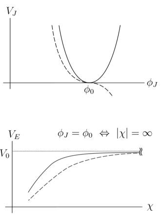
Figure 1: Upper (Lower): A schematic behavior of the Jordan (Einstein)-frame potential around the saddle point $\phi_{0}$ ($\chi=\infty$). Here, the solid (dashed) contour corresponds to $k=$odd (even).

This is schematically shown in the upper panel of Fig.1. In this case, we can expand $V_{J}$ around $\phi_{0}$ as

$$V_{J}(\phi_{J}) =\frac{V_{J}^{(k+1)}}{(k+1)!}(\phi_{J}-\phi_{0})^{k+1}+\frac{V_{J}^{(k+2)}}{(k+2)!}(\phi_{J}-\phi_{0})^{k+2}$$

$$=\frac{|V_{J}^{(k+1)}|\phi_{0}^{k+1}}{(k+1)!}\left(1-\frac{\phi_{J}}{\phi_{0}}\right)^{k+1}$$

$$\times\bigg{(}1+v_{1}^{(k+2)}\left(\frac{\phi_{J}}{\phi_{0}}-1\right)+v_{2}^{(k+3)}\left(\frac{\phi_{J}}{\phi_{0}}-1\right)^{2}\bigg{)},$$ (14)

where

$$v_{1}^{(k+2)}=\frac{\phi_{0}V_{J}^{(k+2)}}{(k+2)V_{J}^{(k+1)}},\ v_{2}^{(k+3)}=\frac{\phi_{0}V_{J}^{(k+3)}}{(k+2)(k+3)V_{J}^{(k+1)}}.$$ (15)

As for the conformal factor $\Omega$, we can consider various possibilities:

$$\Omega(\phi_{J})^{2}= \left(1-\frac{\phi_{J}}{\phi_{0}}\right)^{k+1}\left(1+\sum_{i\geq 0}\omega_{i}\left(1-\frac{\phi_{J}}{\phi_{0}}\right)^{i}\right),$$ (16)

$$\sum_{i\geq 0}\omega_{i}=0,$$ (17)

where the second equation guarantees $\Omega(0)=1$. In this letter, in order to give some concrete inflationary predictions, we consider the following two models:

$$\Omega=\begin{cases}\left(1-\frac{\phi_{J}^{2}}{\phi_{0}^{2}}\right)^{\frac{k+1}{2}}&\text{(Model 1)},\\ \left(1-\frac{\phi_{J}^{4}}{\phi_{0}^{4}}\right)^{\frac{k+1}{2}}&\text{(Model 2)},\end{cases}$$ (18)

which correspond to Model 1 and Model 2 presented in Ref.Jinno:2017lun , respectively. In the case of Model 1, the Einstein-frame potential becomes

$$V_{E}\simeq\frac{|V_{J}^{(k+1)}|\phi_{0}^{k+1}}{(k+1)!2^{k+1}}\bigg{(}1+\left(\frac{k+1}{2}-v_{1}^{(k+2)}\right)\left(1-\frac{\phi_{J}}{\phi_{0}}\right)$$

$$+\left(v_{2}^{(k+3)}-\frac{k+1}{2}v_{1}^{(k+2)}+\frac{(k+1)(k+2)}{8}\right)\left(1-\frac{\phi_{J}}{\phi_{0}}\right)^{2}\bigg{)}$$

$$\simeq V_{0}\left(1+\eta_{\frac{2}{k+1}}\Omega^{\frac{2}{k+1}}+\eta_{\frac{4}{k+1}}\Omega^{\frac{4}{k+1}}\right),$$ (19)

where

$$V_{0}=\frac{|V_{J}^{(k+1)}|\phi_{0}^{k+1}}{(k+1)!2^{k+1}},\ \eta_{\frac{2}{k+1}}=\frac{1}{2}\left(\frac{k+1}{2}-v_{1}^{(k+2)}\right),$$

$$\eta_{\frac{4}{k+1}}=\frac{1}{2^{2}}\left(v_{2}^{(k+3)}-\frac{k+1}{2}v_{1}^{(k+2)}+\frac{(k+1)(k+2)}{8}\right),$$

$$\hskip 170.71652pt(\text{Model 1})$$ (20)

from which we can see that the resultant leading exponent depends on the coefficients of the Jordan-frame potential. In the lower panel of Fig.1, we schematically show the Einstein-frame potential $V_{E}$. Here note that the saddle point $\phi_{0}$ corresponds to $\chi=\infty$ because of the relation $\chi=-M_{pl}\sqrt{3/2}\ln\Omega$. Here, the solid (dashed) contour corresponds to $k=$odd (even). In the case of Model 2, we have

$$V_{0}=\frac{|V_{J}^{(k+1)}|\phi_{0}^{k+1}}{(k+1)!2^{2(k+1)}},\ \eta_{\frac{2}{k+1}}=\frac{1}{4}\left(\frac{3(k+1)}{2}-v_{1}^{(k+2)}\right),$$

$$\eta_{\frac{4}{k+1}}=\frac{1}{4^{2}}\left(v_{2}^{(k+3)}-\frac{3(k+1)}{2}v_{1}^{(k+2)}+\frac{(k+1)(9k+10)}{8}\right),$$

$$\hskip 170.71652pt(\text{Model 2})$$ (21)

Thus, both of the models typically give the leading exponent $n=\frac{2}{(k+1)}$ as long as we do not require a fine-tuning of the coefficients. As a result, the tensor-to-scalar ratio becomes larger when we increase $k$. Note that, in this framework, the coefficient of the leading term in the potential must be negative, $\eta_{\frac{2}{k+1}}<0$, which enables $\chi$ to roll down it. Furthermore, the potential height $V_{0}$ is also constrained by the curvature perturbation

$$A_{s}=\frac{V_{0}}{24\pi^{2}\epsilon M_{pl}^{4}}=2.2\times 10^{-9}\propto\frac{V_{J}^{(k+1)}(\phi_{0})\phi_{0}^{k+1}}{M_{pl}^{4}}.$$ (22)

In Fig.2, we plot the parameter regions obtained from Eq.(22). Here, the $(k+1)$-th derivative $V_{J}^{(k+1)}(\phi_{0})$ is normalized by $\phi_{0}^{k-3}$, and each bands corresponds to each $k$’s. The solid (dashed) contours represent $N=50\ (60)$.

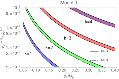
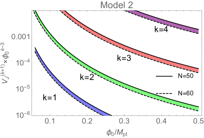
Figure 2: The parameter regions that produce the observed value of the scalar perturbation $A_{s}=2.2\times 10^{-9}$. The upper (lower) panel corresponds to Model 1 (2). Here, the different color bands represent different $k$’s respectively, and the solid (dashed) lines corresponds to $N=50\ (60)$.

In Fig.3, we also show the inflationary predictions obtained from the analytic formulas Eq.(11). Here, the different color lines represent different $k$’s and the small (large) dots correspond to $N=50\ (60)$. Note that $n_{s}$ does not change within this analytic formula because it only depends on the $e$-folding $N$. As is already mentioned in Ref.Jinno:2017lun , the higher order terms of the inflaton potential can have slightly large contributions to the inflationary dynamics, and numerical studies are necessary in order to give more precise predictions. This is left for future investigations.

III Conclusion

In this letter, we have applied the idea of the hillclimbing inflation to the models where the inflaton potential has a saddle point around the Planck scale and shown that it is possible to archive a successful inflation. A notable feature of this class of models is that the leading exponent of the Jordan-frame potential as a function of the conformal factor is typically given by $2/(k+1)$, which leads to a large tensor-to-scalar ratio. Although we have just concentrated on a saddle point of the inflaton potential, we can also consider various realizations of the hillclimbing inflation by using a variety of $V_{J}$ and $\Omega$. So it might be interesting to investigate such possibilities and construct a phenomenological model that can realize a successful inflation.

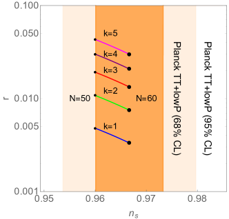
Figure 3: The inflationary predictions of the hillclimbing saddle point inflation. Here, the different color lines represent different $k$’s and the small (large) dots correspond to $N=50\ (60)$.

Acknowledgement

We thank H. Kawai and R.Jinno for valuable comments. The work of KK (KS) is supported by the Grant-in-Aid for JSPS Research Fellow, Grant Number 17J03848 (17J02185).

References

- (1) R. Jinno and K. Kaneta, “Hill-climbing inflation,” Phys. Rev. D 96, no. 4, 043518 (2017) doi:10.1103/PhysRevD.96.043518 [arXiv:1703.09020 [hep-ph]].
- (2) R. Jinno, K. Kaneta and K. y. Oda, “Hillclimbing Higgs inflation,” arXiv:1705.03696 [hep-ph].
- (3) C. D. Froggatt and H. B. Nielsen, “Standard model criticality prediction: Top mass 173 +- 5-GeV and Higgs mass 135 +- 9-GeV,” Phys. Lett. B 368, 96 (1996) doi:10.1016/0370-2693(95)01480-2 [hep-ph/9511371].
- (4) M. Holthausen, K. S. Lim and M. Lindner, “Planck scale Boundary Conditions and the Higgs Mass,” JHEP 1202, 037 (2012) doi:10.1007/JHEP02(2012)037 [arXiv:1112.2415 [hep-ph]].
- (5) F. Bezrukov, M. Y. Kalmykov, B. A. Kniehl and M. Shaposhnikov, “Higgs Boson Mass and New Physics,” JHEP 1210, 140 (2012) doi:10.1007/JHEP10(2012)140 [arXiv:1205.2893 [hep-ph]].
- (6) G. Degrassi, S. Di Vita, J. Elias-Miro, J. R. Espinosa, G. F. Giudice, G. Isidori and A. Strumia, “Higgs mass and vacuum stability in the Standard Model at NNLO,” JHEP 1208, 098 (2012) doi:10.1007/JHEP08(2012)098 [arXiv:1205.6497 [hep-ph]].
- (7) H. B. Nielsen, Bled Workshops Phys. 13, no. 2, 94 (2012) [arXiv:1212.5716 [hep-ph]].
- (8) D. Buttazzo, G. Degrassi, P. P. Giardino, G. F. Giudice, F. Sala, A. Salvio and A. Strumia, “Investigating the near-criticality of the Higgs boson,” JHEP 1312, 089 (2013) doi:10.1007/JHEP12(2013)089 [arXiv:1307.3536 [hep-ph]].
- (9) F. L. Bezrukov and M. Shaposhnikov, “The Standard Model Higgs boson as the inflaton,” Phys. Lett. B 659, 703 (2008) doi:10.1016/j.physletb.2007.11.072 [arXiv:0710.3755 [hep-th]].
- (10) Y. Hamada, H. Kawai, K. y. Oda and S. C. Park, “Higgs inflation from Standard Model criticality,” Phys. Rev. D 91, 053008 (2015) doi:10.1103/PhysRevD.91.053008 [arXiv:1408.4864 [hep-ph]].
- (11) Y. Hamada, H. Kawai and K. Kawana, “Evidence of the Big Fix,” Int. J. Mod. Phys. A 29, 1450099 (2014) doi:10.1142/S0217751X14500997 [arXiv:1405.1310 [hep-ph]].
- (12) Y. Hamada, H. Kawai and K. Kawana, “Weak Scale From the Maximum Entropy Principle,” PTEP 2015, 033B06 (2015) doi:10.1093/ptep/ptv011 [arXiv:1409.6508 [hep-ph]].
- (13) Y. Hamada, H. Kawai and K. Kawana, “Natural solution to the naturalness problem: The universe does fine-tuning,” PTEP 2015, no. 12, 123B03 (2015) doi:10.1093/ptep/ptv168 [arXiv:1509.05955 [hep-th]].
- (14) K. Kawana, “Possible explanations for fine-tuning of the universe,” Int. J. Mod. Phys. A 32, no. 10, 1750048 (2017) doi:10.1142/S0217751X17500488 [arXiv:1609.00513 [hep-th]].
- (15) M. Galante, R. Kallosh, A. Linde and D. Roest, “Unity of Cosmological Inflation Attractors,” Phys. Rev. Lett. 114, no. 14, 141302 (2015) doi:10.1103/PhysRevLett.114.141302 [arXiv:1412.3797 [hep-th]].
- (16) R. Kallosh, A. Linde and D. Roest, “Superconformal Inflationary -Attractors,” JHEP 1311, 198 (2013) doi:10.1007/JHEP11(2013)198 [arXiv:1311.0472 [hep-th]].
- (17) R. Kallosh, A. Linde and D. Roest, “Large field inflation and double -attractors,” JHEP 1408, 052 (2014) doi:10.1007/JHEP08(2014)052 [arXiv:1405.3646 [hep-th]].