AN OPTIMAL ALGORITHM FOR CHANGING FROM LATITUDINAL TO LONGITUDINAL FORMATION OF AUTONOMOUS AIRCRAFT SQUADRONS

?abstractname?

This work presents an algorithm for changing from latitudinal to longitudinal formation of autonomous aircraft squadrons. The maneuvers are defined dynamically by using a predefined set of 3D basic maneuvers. This formation changing is necessary when the squadron has to perform tasks which demand both formations, such as lift off, georeferencing, obstacle avoidance and landing. Simulations show that the formation changing is made without collision. The time complexity analysis of the transformation algorithm reveals that its efficiency is optimal, and the proof of correction ensures its longitudinal formation features.

?abstractname?

Este trabalho apresenta um algoritmo de mudança de formação em latitude para formação longitudinal de esquadrilhas de aeronaves autônomas. As manobras são definidas dinamicamente utilizando-se um conjunto pré-definido de manobras 3D básicas. Esta mudança de formação é necessária quando a esquadrilha tem que desenvolver tarefas que demandam ambas as formações, tais como decolagem, georreferenciamento, desvio de obstáculos e aterrissagem. As simulações mostram que a mudança de formação é feita sem colisão. A análise de complexidade de tempo do algoritmo de transformação revela que sua eficiência é ótima, e a prova de correção assegura suas características de formação longitudinal.

1 Introduction

Recently, it has been possible to see a growing interest in the development of autonomous aircraft that can cooperate with police and other organizations in the solution of public security problems. The basic motivations are: the autonomous agents can deal with dangerous or unhealthy problems, like fires, violence monitoring, inspection of nuclear areas, deforestation monitoring and monitoring of areas with armed conflict, without exposing humans to the risks.

When several agents are used in the solution of these problems, some advantages arise: a) distributed systems are usually more robust than the centralized ones, and b) it is possible to make a better use of sensors, since they can be shared by the network. As an additional example, when autonomous aircraft squadrons are used in georeferencing, the visual field of the cameras increases, as showed in Figure 1, and the captured images can be mosaicked. Besides, autonomous aircraft typically fly at low heights, hence good quality images can be captured.

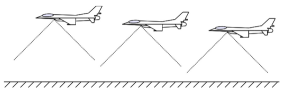
?figurename? 1: The visual field of the aircraft is increased by using squadrons, enabling larger mosaics.

The latitudinal formation presented in Figure 2 is an attractive formation to deal with the georeferencing problem, since better area coverage can be achieved. However, obstacles can appear during the flight, and it may be necessary to change the squadron formation to avoid them. For example, the squadron can assume the longitudinal formation presented in Figure 3 for collision avoidance. Thus, if the first aircraft succeeds in avoiding the collision, all other aircraft in the squadron can also avoid the obstacle by using the same behavior.

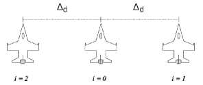
?figurename? 2: The latitudinal formation. It is possible to achieve good area coverage with it.

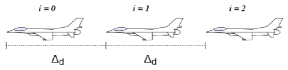
?figurename? 3: The longitudinal formation. It can be used for collision avoidance, landing and lift off.

The longitudinal formation is also necessary when the squadron is landing and doing lift off. Therefore, if the same squadron needs to perform georeferencing, landing, lift off and obstacle avoidance, it will eventually be necessary for the squadron to change between its latitudinal and longitudinal formations.

Therefore, the problem considered in this work is: assuming that there are $n$ aircraft in latitudinal formation, equally spaced by $\Delta_{d}$ meters, we want to develop an algorithm that changes the squadron to the longitudinal formation, where the aircraft will also be equally spaced by $\Delta_{d}$ meters, without collision among them.

This problem involves aircraft formation, trajectory generation and control. The nonlinear model predictive control approach of [Chao] and the leader-follower approach of [You] and [Gu] deal with the formation problem, but changing between well defined geometric formations is not considered. Trajectory generation made by using optimization algorithms are usually found in the literature. Some examples are the works of [Cheng] and [Xu], but works like these do not focus on well defined geometric formations. Other techniques are also used in the trajectory definition, like the geometric moments, controlled via nonlinear gradient [Morbidi], the modern matrix analysis used by [Coker], the combination of the hybrid navigation architecture with the local obstacle avoidance methodology and with the model predictive control [Jansen], the navigation functions [Roussos], and the variation of rapidly-exploring random trees [Neto]. But they also do not consider the changing between well defined geometric formations during the flight. Control techniques, like the reinforcement learning [Santos] do not focus on the changing of formation.

The formation reconfiguration is studied by [Venkataramanan], where the aircraft move their position inside a formation, and the same formation is considered before and after the reconfiguration. The autonomous decision-making architecture [Knoll] also considers this problem, but neither [Venkataramanan] nor [Knoll] consider the transition between different formations. After exhaustive literature searching, it was not found an algorithm that deals with the problem considered here. Thus, the main contributions of this work are:

1. An algorithm for changing from the latitudinal to the longitudinal formation of the squadron. The time complexity analysis of the proposed algorithm shows its efficiency is optimal.

2. A proof of correction of the proposed algorithm, that ensures its longitudinal formation features.

3. The simulation results by considering a case study, in which the aircraft do not collide.

These contributions are described in the next sections, namely: 2 - Methodology, 3 - Simulation Results, 4 - Theoretical Analysis and 5 - Conclusion.

2 Methodology

The proposed algorithm needs to create references to be followed by the aircraft. To do this, a set of maneuvers is specified.

2.1 The Maneuver Schemes

The proposed algorithm employs two 3D basic maneuver schemes, as shown in Figures 4 and 5. For details see [Giacomin-cobem]. Algorithms are used to create the references by using the specifications presented in these figures. Here they are called FW and C to implement the go forward and to turn maneuvers, respectively. The go forward interface is FW($P$, $\varphi$, $\beta$, $vel$, $d$, $T$) and the to turn interface is C($P$, $\varphi$, $\beta$, $\theta$, $\alpha$, $vel$, $r$, $T$), where $P$ is the initial position $(x_{0},y_{0},h_{0})$, $T$ is a vector time to be filled with time intervals, and the other parameters are shown in Figures 4 and 5. These algorithms are used by the transition algorithm described at Subsection 2.2.

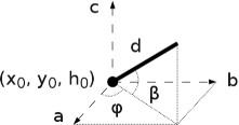
?figurename? 4: Go forward maneuver: two angles, a point and a distance are specified, with $\vec{a}\parallel\vec{x}$, $\vec{b}\parallel\vec{y}$ and $\vec{c}\parallel\vec{h}$.

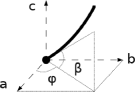
(a) Part a

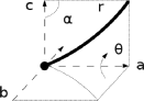
(b) Part b

?figurename? 5: To turn maneuver: four angles, a 3D point and a radius need to be specified.

2.2 The Transition Algorithm

The transition algorithm is shown in Algorithm 1. It is called FLATLO due to the initial characters that describe its function: From Latitudinal To Longitudinal formation. It basically performs the maneuvers presented in Figure 6 by each aircraft on the left of the squadron, and the equivalent mirrored one for each aircraft on the right of the squadron.

Algorithm 1 The transition algorithm

1:procedure FLATLO($i$, $\Delta_{d}$, $vel$, $r$, $\varphi$, $\beta$, $P$)

2:     $T\leftarrow\varnothing$

3:     $Ref\leftarrow\varnothing$

4:     $\Delta_{m}\leftarrow move\_forward(i,\Delta_{d})$

5:     $side\leftarrow get\_side(i,N)$

6:     $a\leftarrow FW(P,\varphi,\beta,vel,\Delta_{m},T)$

7:     $Ref\leftarrow Ref\cup a$

8:     if $|Ref|\neq 0$ then

9:         $P_{1}\leftarrow last(Ref)$

10:     else

11:         $P_{1}\leftarrow P$

12:     end if

13:     $k\leftarrow 0$

14:     while $k<4$ do

15:         if $|Ref|\neq 0$ then

16:              $P_{1}\leftarrow last(Ref)$

17:              $P_{0}\leftarrow penultimate(Ref)$

18:              $D\leftarrow distance(P_{1},P_{0})$

19:              $\varphi_{2}\leftarrow sin^{-1}(\Delta_{y}/D)$

20:              $\beta_{2}\leftarrow sin^{-1}(\Delta_{h}/D)$

21:         else

22:              $\varphi_{2}=\varphi$

23:              $\beta_{2}=\beta$

24:         end if

25:         if $k=0$ then

26:              if $side=LEFT$ then

27:                  $a\leftarrow C(P_{1},\varphi_{2},\beta_{2},\pi,\frac{\pi}{4},vel,r,T)$

28:              else

29:                  $a\leftarrow C(P_{1},\varphi_{2},\beta_{2},0,\frac{\pi}{4},vel,r,T)$

30:              end if

31:         else if $k=1$ then

32:              if $even(N)$ then

33:                  $\Delta\leftarrow\Delta_{d}/2+\lfloor i/2\rfloor\cdot\Delta_{d}$

34:              else

35:                  if $i\neq 0$ then

36:                       $\Delta\leftarrow\Delta_{d}\cdot\lfloor(i+1)/2\rfloor$

37:                  else

38:                       $\Delta\leftarrow 0$

39:                  end if

40:              end if

41:              $\Delta_{2}\leftarrow\sqrt{2}\cdot(\Delta-2\cdot r\cdot(1-cos(\pi/4)))$

42:              $a\leftarrow FW(P_{1},\varphi_{2},\beta_{2},vel,\Delta_{2},T)$

43:         else if $k=2$ then

44:              if $side=LEFT$ then

45:                  $a\leftarrow C(P_{1},\varphi_{2},\beta_{2},0,\frac{\pi}{4},vel,r,T)$

46:              else

47:                  $\varphi_{3}\leftarrow-\varphi_{2}$

48:                  $a\leftarrow C(P_{1},\varphi_{3},\beta_{2},\pi,\frac{\pi}{4},vel,r,T)$

49:              end if

50:         else

51:              $a\leftarrow FW(P_{1},\varphi_{2},\beta_{2},vel,K_{2},T)$

52:         end if

53:         $Ref\leftarrow Ref\cup a$

54:         $k\leftarrow k+1$

55:     end while

56:     return $Ref$

57:end procedure

Algorithm 2 The advancing algorithm

1:procedure move_forward($i$, $\Delta_{d}$)

2:     if $odd(N)$ then

3:         if $odd(i)$ then

4:              $k\leftarrow\lfloor(N-i)/2\rfloor$

5:              $\Delta_{m}\leftarrow k\cdot\Delta_{d}+2\cdot(k-1)\cdot\Delta_{d}$

6:         else

7:              $\Delta_{m}\leftarrow 3\cdot\Delta_{d}\cdot\lfloor(N-i-1)/2\rfloor$

8:         end if

9:     else

10:         if $odd(i)$ then

11:              $\Delta_{m}\leftarrow 3\cdot\Delta_{d}\cdot\lfloor(N-i-1)/2\rfloor$

12:         else

13:              $k\leftarrow\lfloor(N-i)/2\rfloor$

14:              $\Delta_{m}\leftarrow k\cdot\Delta_{d}+2\cdot(k-1)\cdot\Delta_{d}$

15:         end if

16:     end if

17:     return $\Delta_{m}$

18:end procedure

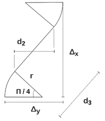
?figurename? 6: An aircraft goes to the middle of squadron when it assumes the longitudinal formation.

The interface of the transition algorithm is FLATLO($i$, $\Delta_{d}$, $vel$, $r$, $\varphi$, $\beta$, $P$), where $i$ is the aircraft index shown in Figures 2 and 3, $vel$ is the aircraft airspeed, $r$ is the radius of the to turn maneuvers used by the transition algorithm, $\varphi$ and $\beta$ are shown in Figure 5a, and $P$ is the aircraft initial position $(x_{0},y_{0},h_{0})$.

Algorithm 1 is executed by each aircraft processor, in parallel. For all aircraft, except the last one, it is calculated the forward displacement, called $\Delta_{m}$, at Line 4. See Algorithm 2 for details. Thereafter, each aircraft executes four maneuvers. The values that are determined between Lines 15 and 24 are used to fit each maneuver with the next one.

Each aircraft moves in direction to the longitudinal line of the squadron between Lines 26 and 30. At Line 42, the aircraft goes forward in direction to the longitudinal line. Between Lines 44 and 49, the aircraft moves to enter smoothly on the longitudinal line. Finally, the aircraft flies over the longitudinal line at Line 51.

The references created by the Algorithm 1 were tested by using the aircraft model presented at Subsection 2.3.

2.3 The Aircraft Model

The simple and well-tested aircraft state space model, [Anderson], is employed, and is given by

$$\frac{dV}{dt}=g\cdot\left[\frac{(T-D)}{W}-sin(\gamma)\right]$$ (1)

$$\frac{d\gamma}{dt}=\frac{g}{V}\cdot[n\cdot cos(\mu)-cos(\gamma)]$$ (2)

$$\frac{d\chi}{dt}=\frac{g\cdot n\cdot sin(\mu)}{V\cdot cos(\gamma)}$$ (3)

$$\frac{dx}{dt}=V\cdot cos(\gamma)\cdot cos(\chi)$$ (4)

$$\frac{dy}{dt}=V\cdot cos(\gamma)\cdot sin(\chi)$$ (5)

$$\frac{dh}{dt}=V\cdot sin(\gamma)$$ (6)

where the state variables are: airspeed (V), flight path angle ($\gamma$), flight path heading ($\chi$), and the position variables (x, y, h).

A control scheme is presented in [Giacomin-cobem] by using the above aircraft model. Here, the references created by Algorithm 1 are submitted to this control scheme.

3 Simulation Results

The Algorithm 1 is programmed in parallel by using the C++ programming language and the GNU Message Passing Interface (MPI) Compiler. It is allocated one processor for each aircraft. The graphics are plotted by using the software Gnuplot.

The initial condition for all aircraft are: height: $3,050.00$ meters, airspeed: $30.5$ m/s, $\Delta_{d}=18,300.00$ meters, assuming the latitudinal formation. The references are created by Algorithm 1 by using radius of $4,575.00$ meters, and different airspeeds for each aircraft, that allow all aircraft to arrive on longitudinal formation at the same time instant. The simulation is made by using the Runge-Kutta-4 algorithm. The results are shown in Figures 7, 8 and 9.

?figurename? 7: The aircraft references. The marks are used in the aircraft crossing analysis.

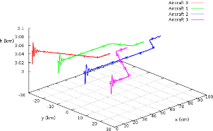
?figurename? 8: The aircraft trajectories. The aircraft succeed in following the references.

The marks shown in Figures 7 and 8 are used to analyze the aircraft crossing. When the aircraft number zero is flying over the third mark, the aircraft number one is ahead, and when aircraft number tree is flying over fourth mark, the aircraft number two is ahead. An automatic verification did show that the minimum distance between aircraft $0$ and $1$ and between aircraft $2$ and $3$ was $14.5$ km and $18.3$ km, respectively. Therefore, there is no collision.

The simulation is made by considering a noise of $0,25\%$ for airspeed, heading and gamma angles. From Figures 7, 8 and 9 it is possible to conclude that Algorithm 1 creates the references correctly and that the aircraft succeed in following the references.

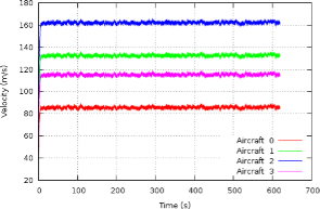
?figurename? 9: All aircraft velocities.

It remains to analyze the time complexity of the Algorithm 1 and to prove its correction. This is made in Section 4.

4 Theoretical Analysis

The theoretical analysis of Algorithm 1 is divided into two parts: its time complexity analysis and its proof of correction.

4.1 The Time Complexity Analysis

The go forward and to turn functions are executed over a fixed number of maneuvers, and all other functions used in Algorithm 1 have constant time complexity. Let $Q=\{q_{0},\cdots,q_{|Q|-1}\}$ be the set of maneuvers, and let $R=\{r_{0},\cdots,r_{|Q|-1}\}$ be the set of references, with $r_{i}=ref(q_{i})$, and the function ref be implemented by using the functions FW or C in the Algorithm 1. Then, $R$ is a set of sets, and $|r_{i}|$ is the references quantity for each maneuver $q_{i}$. The time complexity of Algorithm 1 is

$$O(|r_{0}|+|r_{1}|+|r_{2}|+|r_{3}|+|r_{4}|)$$

$$m=|r_{0}|+\cdots+|r_{4}|$$

$$O(m)$$

where $m$ represents the total time steps for each aircraft trajectory. Since this is also the lower bound for the problem, it is concluded that the FLATLO algorithm is optimal with regard to the time complexity [Cormen].

4.2 The Proof of Correction

The proof of correction takes into account that the maneuvers executed by Algorithm 1 are basically described in Figure 6, except the first one, that is created by Algorithm 2.

Note that when an aircraft on latitudinal formation advances the distance $\Delta_{d}$ before executing the trajectory of Figure 6, $\Delta_{x}$ advances $\Delta_{d}$ on its longitudinal formation. This information is used in the proof of the next theorem.

Theorem 4.1

Let assume a set of aircraft initially flying in latitudinal formation, with each aircraft equally spaced by $\Delta_{d}$ from its neighbors. Then, if the FLATLO algorithm is executed by each aircraft, the longitudinal formation, with spacing $\Delta_{d}$ between its neighbors, is achieved.

Proof 4.2

It is considered $n$ aircraft in the squadron. Clearly, if $n$ is even and $i$ is even, it can be concluded by analyzing Algorithm 2 that $\Delta_{m}^{i}-\Delta_{m}^{i+1}=\Delta_{d}$. Then

$$\Delta_{x}^{i}=k\cdot\Delta_{d}+2\cdot r\cdot sin(\pi/4)+\Delta_{y}-2\cdot r\cdot(1-cos(\pi/4))$$

$$\Delta_{x}^{i+1}=(k-1)\cdot\Delta_{d}+2\cdot r\cdot sin(\pi/4)+\Delta_{y}-\cdots$$

$$\cdots-2\cdot r\cdot(1-cos(\pi/4))$$

$$\Delta_{x}^{i}-\Delta_{x}^{i+1}=\Delta_{d}$$

that is the obvious case where the two aircraft $i$ and $i+1$ are mirrored by the middle line. If $i$ is odd, it follows, by analyzing Algorithm 2, that $\Delta_{m}^{i}-\Delta_{m}^{i+1}=2\cdot\Delta_{d}$. Then

$$\Delta_{x}^{i}=k\cdot\Delta_{d}+2\cdot r\cdot sin(\pi/4)+\Delta_{y}-2\cdot r\cdot(1-cos(\pi/4))$$

$$\Delta_{x}^{i+1}=(k-2)\cdot\Delta_{d}+2\cdot r\cdot sin(\pi/4)+(\Delta_{d}+\Delta_{y})-\cdots$$

$$\cdots-2\cdot r\cdot(1-cos(\pi/4))$$

$$\Delta_{x}^{i}-\Delta_{x}^{i+1}=k\cdot\Delta_{d}-(k-2)\cdot\Delta_{d}-\Delta_{d}$$

$$\Delta_{x}^{i}-\Delta_{x}^{i+1}=\Delta_{d}$$

On the other hand, if $n$ is odd and $i$ is even, it follows, by analyzing Algorithm 2, that $\Delta_{m}^{i}-\Delta_{m}^{i+1}=2\cdot\Delta_{d}$, that is the same case that happens when $n$ is even and $i$ is odd. If $n$ is odd and $i$ is odd, then it follows, by analyzing Algorithm 2, that $\Delta_{m}^{i}-\Delta_{m}^{i+1}=\Delta_{d}$, which has the same result obtained when $n$ is even and $i$ is even. Therefore, $\Delta_{x}^{i}-\Delta_{x}^{i+1}=\Delta_{d}$ for every $n$ and for every $i$.

Similar reasoning can be applied to $\Delta_{y}$. Lines 32 to 40 show that $\Delta^{i+2}-\Delta^{i}=\Delta_{d}$, for every $n$ and every $i$. Then, if $n$ is even

$$\Delta_{y}^{i}=2\cdot r\cdot(1-cos(\pi/4))+\Delta_{d}/2+k\cdot\Delta_{d}+\Delta_{x}-\cdots$$

$$\cdots-2\cdot r\cdot sin(\pi/4)$$

$$\Delta_{y}^{i+2}=2\cdot r\cdot(1-cos(\pi/4))+\Delta_{d}/2+\Delta_{d}+\cdots$$

$$\cdots+(k-1)\cdot\Delta_{d}+\Delta_{x}-2\cdot r\cdot sin(\pi/4)$$

$$\Delta_{y}^{i+2}-\Delta_{y}^{i}=0$$

and if $n$ if odd it follows that

$$\Delta_{y}^{i}=2\cdot r\cdot(1-cos(\pi/4))+k\cdot\Delta_{d}+\Delta_{x}-\cdots$$

$$\cdots-2\cdot r\cdot sin(\pi/4)$$

$$\Delta_{y}^{i+2}=2\cdot r\cdot(1-cos(\pi/4))+\Delta_{d}+(k-1)\cdot\Delta_{d}+\cdots$$

$$\cdots+\Delta_{x}-2\cdot r\cdot sin(\pi/4)$$

$$\Delta_{y}^{i+2}-\Delta_{y}^{i}=0$$

and therefore, $\Delta_{y}^{i+2}-\Delta_{y}^{i}=0$ for every $n$ and for every $i$. Since this same reasoning can be made for other coordinate system bases, and since all aircraft arrive on longitudinal formation at the same time instant, then the proof follows.

5 Conclusion

An algorithm for changing from latitudinal to longitudinal formation for autonomous aircraft squadrons is proposed in this paper. Despite the relevance of this problem, extensive literature review did not produce relevant results.

The proposed FLATLO algorithm time complexity is equal to the problem lower bound, hence it is optimal [Cormen].

It was proved that if the squadron is initially on latitudinal formation, with each aircraft equally spaced from its neighbors by distance $\Delta_{d}$, then the proposed algorithm makes the squadron to change its formation to longitudinal one, keeping the same distance $\Delta_{d}$ from each aircraft and its neighbors.

The theoretical analysis was confirmed by the simulations, by showing that the aircraft do not collide during the formation transition, and that the references were created correctly by the proposed algorithm, such that they could be followed by a control scheme. Additionally, since the aircraft use different velocities, the number of aircraft has to be limited, and the velocities have to be verified at design time, for security reasons.

- [1] \harvarditemAnderson \harvardand Robbins1998Anderson Anderson, M. R. \harvardand Robbins, A. C. \harvardyearleft1998\harvardyearright. Formation flight as a cooperative game, Collection of Technical AIAA Guidance, Navigation, and Control Conference and Exhibit 10(12): 244–251.
- [2] \harvarditem[Chao et al.]Chao, Zhou, Ming \harvardand Zhang2012Chao Chao, Z., Zhou, S.-L., Ming, L. \harvardand Zhang, W.-G. \harvardyearleft2012\harvardyearright. Uav formation flight based on nonlinear model predictive control, Mathematical Problems in Engineering 2012(261367): 1–15.
- [3] \harvarditemCheng \harvardand Leung2012Cheng Cheng, C. \harvardand Leung, H. \harvardyearleft2012\harvardyearright. A genetic algorithm-inspired uuv path planner based on dynamic programming, IEEE Transactions on Systems, Man and Cybernetics – Part C: Applications and Reviews 42(6): 1128–1134.
- [4] \harvarditemCoker \harvardand Tewfik2011Coker Coker, J. \harvardand Tewfik, A. \harvardyearleft2011\harvardyearright. Performance synthesis of uav trajectories in multistatic sar, Aerospace and Electronic Systems, IEEE Transactions on 47(2): 848–863.
- [5] \harvarditem[Cormen et al.]Cormen, Leiserson, Rivest \harvardand Stein2009Cormen Cormen, T. H., Leiserson, C. E., Rivest, R. L. \harvardand Stein, C. \harvardyearleft2009\harvardyearright. Introduction to Algorithms, MIT Press.
- [6] \harvarditemGiacomin \harvardand Hemerly2013Giacomin-cobem Giacomin, P. A. S. \harvardand Hemerly, E. M. \harvardyearleft2013\harvardyearright. Parallel simulation for autonomous aircrafts squadrons using virtual structure and a 3d maneuvers scheme, 22nd International Congress of Mechanical Engineering, Submitted.
- [7] \harvarditem[Gu et al.]Gu, Campa \harvardand Seanor2009Gu Gu, Y., Campa, G. \harvardand Seanor, B. \harvardyearleft2009\harvardyearright. Aherial Vehicles, InTech, chapter Autonomous formation flight - desing and experiments, pp. 235–257.
- [8] \harvarditemJansen \harvardand Ramirez-Serrano2011Jansen Jansen, F. \harvardand Ramirez-Serrano, A. \harvardyearleft2011\harvardyearright. Agile unmanned vehicle navigation in highly confined environments, IEEE International Conference on Systems, Man, and Cybernetics, p. 2381–2386.
- [9] \harvarditemKnoll \harvardand Beck2006Knoll Knoll, A. \harvardand Beck, J. \harvardyearleft2006\harvardyearright. Autonomous decision-making applied onto uav formation flight, AIAA Modeling and Simulation Technologies Conference and Exhibit.
- [10] \harvarditem[Morbidi et al.]Morbidi, Freeman \harvardand Lynch2011Morbidi Morbidi, F., Freeman, R. \harvardand Lynch, K. \harvardyearleft2011\harvardyearright. Estimation and control of uav swarms for distributed monitoring tasks, American Control Conference (ACC), 2011, pp. 1069–1075.
- [11] \harvarditem[Neto et al.]Neto, Macharet \harvardand Campos2010Neto Neto, A. A., Macharet, D. G. \harvardand Campos, M. F. \harvardyearleft2010\harvardyearright. On the generation of trajectories for multiple uavs in environments with obstacles, J. Intell. Robotics Syst. 57(1-4): 123–141.
- [12] \harvarditemRoussos \harvardand Kyriakopoulos2012Roussos Roussos, G. \harvardand Kyriakopoulos, K. J. \harvardyearleft2012\harvardyearright. Decentralized navigation and conflict avoidance for aircraft in 3-d space, IEEE Transactions on Control Systems Technology 20(6): 1622 – 1629.
- [13] \harvarditem[Santos et al.]Santos, Givigi \harvardand Nascimento Junior2012Santos Santos, S. B. d., Givigi, S. \harvardand Nascimento Junior, C. \harvardyearleft2012\harvardyearright. An experimental validation of reinforcement learning applied to the position control of uavs, Systems, Man, and Cybernetics (SMC), 2012 IEEE International Conference on, pp. 2796–2802.
- [14] \harvarditemVenkataramanan \harvardand Dogan2004Venkataramanan Venkataramanan, S. \harvardand Dogan, A. \harvardyearleft2004\harvardyearright. A multi-uav simulation for formation reconfiguration, AIAA Modeling and Simulation Technologies Conference and Exhibit.
- [15] \harvarditem[Xu et al.]Xu, Kang, Cai \harvardand Chen2012Xu Xu, N., Kang, W., Cai, G. \harvardand Chen, B. M. \harvardyearleft2012\harvardyearright. Minimum-time trajectory planning for helicopter uavs using computational dynamic optimization, IEEE International Conference on Systems, Man and Cybernetics, pp. 2732–2737.
- [16] \harvarditemYou \harvardand Shim2011You You, D. I. \harvardand Shim, D. H. \harvardyearleft2011\harvardyearright. Autonomous formation flight test of multi-micro aerial vehicles, J Intell Robot Syst 61(1-4): 321–337.
- [17]