Abstract

We present a comprehensive analysis of the muon magnetic moment $a_{\mu}$ in the flavour-aligned two-Higgs doublet model (2HDM) and parameter constraints relevant for $a_{\mu}$. We employ a recent full two-loop computation of $a_{\mu}$ and take into account experimental constraints from Higgs and flavour physics on the parameter space. Large $a_{\mu}$ is possible for light pseudoscalar Higgs $A$ with large Yukawa couplings to leptons, and it can be further increased by large $A$ coupling to top quarks. We investigate in detail the maximum possible Yukawa couplings to leptons and quarks of a light $A$, finding values of around $50\ldots 100$ (leptons) and ${\cal O}(0.5)$ (quarks). As a result we find that an overall maximum of $a_{\mu}$ in the 2HDM of more than $45\times 10^{-10}$ is possible in a very small parameter region around $M_{A}=20$ GeV. The parameter regions in which the currently observed deviation can be explained are characterized.

1 Introduction

The two-Higgs doublet model (2HDM) is one of the most common extensions of the Standard Model (SM). It is the simplest model with non-minimal electroweak symmetry breaking, comprising two SU(2) doublets and five physical Higgs bosons $h$, $H$, $A$, $H^{\pm}$, where $h$ must be SM-like to agree with LHC-data. The extra Higgs bosons are actively searched for at the LHC.

For more than a decade the measured value [1] of the anomalous magnetic moment of the muon $a_{\mu}=(g-2)_{\mu}/2$ has shown a persisting deviation from the current SM prediction (for recent developments see Refs. [2, 3, 4, 5] (QED and electroweak corrections), [6, 7, 8, 9, 10, 11, 12, 13, 14, 15, 16, 17, 18, 19] (QCD corrections)). Using the evaluation of the indicated references, the current deviation is

$$a_{\mu}^{\text{Exp$-$SM}} =\begin{cases}(26.8\pm 7.6)\times 10^{-10}\mbox{\cite[cite]{[\@@bibref{}{Davier}{}{}]}},\\ (28.1\pm 7.3)\times 10^{-10}\mbox{\cite[cite]{[\@@bibref{}{KNTTalks}{}{}]}},\\ (31.3\pm 7.7)\times 10^{-10}\mbox{\cite[cite]{[\@@bibref{}{Jegerlehner:2017lbd}{}{}]}}.\end{cases}$$ (1)

$a_{\mu}$ provides a tantalizing hint for new physics. The hint might be strongly sharpened by a new generation of $a_{\mu}$ measurements at Fermilab and J-PARC [20, 21]. Hence it is of high interest to identify new physics models which are able to explain the current deviation, or a future larger or smaller deviation.

Recently it has been repeatedly stressed that the 2HDM is such a model. This is a non-trivial observation since the leading 2HDM contributions to $a_{\mu}$ arise only at the two-loop level and small Higgs masses are needed to compensate the two-loop suppression. Specifically, Refs. [22, 24, 25, 26, 27, 23] have studied the so-called type X (or lepton-specific) model, Refs. [29, 28, 30] the more general (flavour-)aligned model [31, 32]. In all these cases it was shown that a light pseudoscalar $A$ boson with large couplings to leptons is viable and could explain Eq. (1) or at least most of it. Ref. [28] has also found an additional small parameter region with very light scalar $H$; furthermore, Ref. [33] has studied a $Z_{4}$-symmetric, “muon-specific” model which can explain Eq. (1) for $\tan\beta\sim 1000$.

At the same time, the accuracy of the $a_{\mu}$ prediction in the 2HDM has increased. Ref. [30] has computed the 2HDM contributions fully at the two-loop level, including all bosonic contributions (from Feynman diagrams without closed fermion loop). Prior to that, Ref. [29] had computed all contributions of the Barr-Zee type [34]. As a result of these calculations, the 2HDM theory uncertainty is fully under control and significantly below the theory uncertainty of the SM prediction and the resolution of the future $a_{\mu}$ measurements.

Here we employ the full two-loop prediction to carry out a detailed phenomenological study of $a_{\mu}$ in the general flavour-aligned 2HDM and of the parameters relevant for $a_{\mu}$. In detail, the questions we consider are

• What are the constraints on the 2HDM parameters most relevant for $a_{\mu}$ (the mass of the $A$ boson and its Yukawa couplings to leptons and quarks, and further 2HDM masses and Higgs potential parameters)?

• In which parameter region can the 2HDM accommodate the current deviation in $a_{\mu}$ (or a future, possibly larger or smaller deviation)?

• What is the overall maximum possible value of $a_{\mu}$ that can be obtained in the 2HDM (for various choices of restrictions on the Yukawa couplings)?

We will generally focus on the promising scenario with $M_{A}<M_{h}$ and allow for general flavour-aligned Yukawa couplings but will comment also on the more restrictive case of the lepton-specific type X model. We will take into account constraints from theoretical considerations such as tree-level unitarity and perturbativity, experimental constraints from collider data from LHC and LEP, and constraints from B- and $\tau$-physics.

The outline of the paper is as follows. In section 2, we describe our setup and give details on the definition of the 2HDM. Section 3 then discusses the detailed constraints on the parameters most relevant for $a_{\mu}$ in the 2HDM: on the Higgs masses, on the Yukawa couplings, and on Higgs potential parameters and Higgs self couplings. Section 4 gives an updated discussion of the full bosonic two-loop contributions, taking into account detailed constraints on the parameters. Section 5 finally gives the results on $a_{\mu}$ in the 2HDM. The results are presented both as contour plots in parameter planes, and as plots showing the maximum possible values of $a_{\mu}$ in the 2HDM.

2 Setup

In this section we provide the basic relations for the two-Higgs doublet model (2HDM) and describe our technical setup.

2.1 Definition of the 2HDM

We use the 2HDM with general Higgs potential in the notation of Ref. [35, 36],

$$V\left(\phi_{1},\phi_{2}\right) =m^{2}_{11}\phi^{\dagger}_{1}\phi_{1}+m^{2}_{22}\phi^{\dagger}_{2}\phi_{2}-\{m^{2}_{12}\phi^{\dagger}_{1}\phi_{2}+{\text{H.c.}}\}$$

$$+\frac{\lambda_{1}}{2}(\phi^{\dagger}_{1}\phi_{1})^{2}+\frac{\lambda_{2}}{2}(\phi^{\dagger}_{2}\phi_{2})^{2}+\lambda_{3}(\phi^{\dagger}_{1}\phi_{1})(\phi^{\dagger}_{2}\phi_{2})$$

$$+\lambda_{4}(\phi^{\dagger}_{1}\phi_{2})(\phi^{\dagger}_{2}\phi_{1})+\frac{1}{2}\left\{\lambda_{5}(\phi^{\dagger}_{1}\phi_{2})^{2}+{\text{H.c.}}\right\}$$

$$+\left\{[\lambda_{6}(\phi^{\dagger}_{1}\phi_{1})+\lambda_{7}(\phi^{\dagger}_{2}\phi_{2})]\phi^{\dagger}_{1}\phi_{2}+{\text{H.c.}}\right\}.$$ (2)

In the usual type I, II, X, Y models a $Z_{2}$ symmetry is assumed which enforces the two parameters $\lambda_{6}$ and $\lambda_{7}$ to vanish. In the following we will investigate both the case with $\lambda_{6}=\lambda_{7}=0$ and the case with non-vanishing $\lambda_{6},\lambda_{7}$. Since we focus on the muon magnetic moment, which is not enhanced by CP violation, we assume all parameters to be real. In the minimum of the potential the two Higgs doublets acquire the vacuum expectation values (VEVs) $v_{1,2}$ with the ratio $\tan\beta=v_{2}/v_{1}$. It is then instructive to rotate the doublets by the angle $\beta$ to the so-called Higgs basis [35], in which one doublet has the full SM-like VEV $v=\sqrt{v_{1}^{2}+v_{2}^{2}}$ and the other doublet has zero VEV. The second doublet then contains the physical CP-odd Higgs $A$ and the charged Higgs $H^{\pm}$, and the physical CP-even Higgs fields $h,H$ correspond to mixtures between the two doublets in the Higgs basis with mixing angle $(\alpha-\beta)$. In practice we will choose the following set of independent input parameters:

$$M_{h,H,A,H^{\pm}},\tan\beta,c_{\beta\alpha},\lambda_{1},\lambda_{6},\lambda_{7},$$ (3)

where $c_{\beta\alpha}\equiv\cos(\beta-\alpha)$ and similar for $s_{\beta\alpha}$. We will further choose $h$ to be the approximately SM-like Higgs state, which means that the mass $M_{h}$ is fixed to the observed value of $125$ GeV and that the mixing angle $c_{\beta\alpha}$ is small. It should be noted that all parameters in this list enter the prediction of the muon $g-2$ only at the two-loop level and hence do not have to be renormalized.

For the Yukawa couplings we choose the setup of the (flavour-)aligned 2HDM of Ref. [31]. In this setup one assumes the following structure of the Yukawa couplings in the Higgs basis: the SM-like doublet has SM-like Yukawa couplings by construction; the other doublet has couplings proportional to the SM-like ones, with proportionality factors $\zeta_{l}$ (for charged leptons), $\zeta_{u,d}$ (for up- and down-type quarks). For the mass-eigenstate Higgs bosons this implies the following Yukawa Lagrangian:

$${\cal{L}}_{Y}= -\frac{\sqrt{2}}{v}H^{+}\Big{(}{\bar{u}}[\zeta_{d}V_{\text{CKM}}M_{d}P_{\text{R}}-\zeta_{u}M_{u}V_{\text{CKM}}P_{\text{L}}]d+\zeta_{l}{\bar{\nu}}M_{l}P_{\text{R}}l\Big{)}$$

$$-\sum_{{{\cal S}=h,H,A}}\sum_{{f=u,d,l}}\,{\cal S}{\bar{f}}y_{f}^{\cal S}P_{\text{R}}f+{\text{H.c.}},$$ (4)

where $P_{{\text{R}},{\text{L}}}=\frac{1}{2}(1\pm\gamma_{5})$, and $V_{\text{CKM}}$ is the Cabibbo-Kobayashi-Maskawa matrix. $M_{f}$ denotes the diagonal $3\times 3$ mass matrices. The Yukawa coupling matrices are defined as

$$y_{f}^{\cal S} =\frac{Y_{f}^{\cal S}}{v}M_{f},$$ (5)

where

$$Y^{h}_{f} =s_{\beta\alpha}+c_{\beta\alpha}\zeta_{f},$$

$$Y^{H}_{f} =c_{\beta\alpha}-s_{\beta\alpha}\zeta_{f},$$

$$Y^{A}_{d,l} =i\zeta_{d,l},$$

$$Y^{A}_{u} =-i\zeta_{u}.$$ (6)

The flavour-aligned 2HDM contains the usual type I, II, X, Y models as special cases, see table 1. Most notably, in type II, the product $|\zeta_{u}\zeta_{d}|=\cot\beta\;\tan\beta=1$ is never small, implying very strong constraints from $b\to s\gamma$ for all values of $\tan\beta$ [37]. And in type X, $\zeta_{l}=-\tan\beta$ and $\zeta_{u}=\zeta_{d}=\cot\beta$ cannot be simultaneously large.

	Type I	Type II	Type X	Type Y
$\zeta_{u}$	$\cot\beta$	$\cot\beta$	$\cot\beta$	$\cot\beta$
$\zeta_{d}$	$\cot\beta$	$-\tan\beta$	$\cot\beta$	$-\tan\beta$
$\zeta_{l}$	$\cot\beta$	$-\tan\beta$	$-\tan\beta$	$\cot\beta$

Table 1: Relation between the Yukawa parameters $\zeta_{f}$ in the general, aligned 2HDM and the usual type I, II, X, and Y models.

As shown in Refs. [32, 38] the flavour-aligned scenario is minimal flavour violating and even though the alignment is not strictly protected by a symmetry, it is numerically rather stable under renormalization-group running. Hence we regard it as a theoretically and phenomenologically well motivated and very general scenario.

2.2 Technical remarks

In order to check the viability of parameter points against experimental and theoretical constraints, we have adopted the routines implemented in the 2HDMC code [39], which allows checks regarding theoretical constraints such as stability, unitarity, and perturbativity of the quartic couplings; the S, T, U precision electroweak parameters; and data from colliders implemented in the HiggsBounds and HiggsSignals packages [40, 41].

For our later scans of parameter space we started with a wide range of all Higgs potential parameters in Eq. (3) and the Yukawa parameters $\zeta_{l,u,d}$. This range was narrowed down to

$$\zeta_{d} =-0.7\ldots 1.1, \lambda_{1} =0\ldots 2\pi,$$

$$\lambda_{6} =-2\ldots 2, \lambda_{7} =-3\ldots 3,$$ (7)

$$\tan\beta =0.3\ldots 2, |c_{\beta\alpha}| <1/|\zeta_{l}|,$$

after checking that this covers the parameter space with the largest possible contributions to all quantities of interest. Unless specified differently, these are the parameter ranges used in our scatter plots. In the plots evaluating $a_{\mu}$, in addition we set $\zeta_{d}=0$ to be specific, because this parameter has a very small influence on $a_{\mu}$.

Regarding statistics, we have adopted the following procedure: first we constructed a $\chi^{2}$ distribution for the physical process under consideration, and then computed its respective p-value distribution, assuming that the errors are gaussian and robust as usual [42]. Finally, we required that the p-value for the considered observable (or set of observables) is greater than 0.05 (corresponding to a 95% CL region). For the constraints to be discussed in Sec.3.2, this approach is slightly different from the one implemented in Ref. [23], but we checked that the resulting exclusion contours are very similar.

3 Constraints

In this section we provide a detailed investigation of experimental constraints on the 2HDM parameter space with general flavour-aligned Yukawa couplings. Earlier studies [22, 24, 29, 25, 26, 27, 28, 23, 30] and our later considerations show that $a_{\mu}$ can be promisingly large for small $M_{A}$ and large $\zeta_{l}$ and $\zeta_{u}$, so we focus on this scenario. Our study can be regarded as a generalization of Refs. [22, 23, 25], which focused on the lepton-specific (type X) case, where $\zeta_{u}=-1/\zeta_{l}=1/\tan\beta$, and as complementary to Ref. [28], which focused on correlations in scans of parameter space. Our questions are: what are the maximum values of $\zeta_{l}$ and $\zeta_{u}$ and other relevant parameters, and how do these maximum values depend on the value of the small Higgs mass $M_{A}$ or the heavy Higgs masses?

We will begin with the most direct and basic constraints on the scenario with small $M_{A}$ from collider physics, then focus on maximum possible values of $\zeta_{l}$ and $\zeta_{u}$ and correlated parameters.

3.1 Basic collider constraints on small $M_{A}$ and on mixing angle $\cos(\beta-\alpha)$

The scenario with light CP-odd Higgs boson $A$ is obviously strongly constrained by collider physics. The most immediate constraints arise from negative results of direct $A$ searches. On the one hand these results imply upper limits of the couplings between the $A$ and $W$ and $Z$ bosons and thus on the mixing angle $c_{\beta\alpha}$. However, below we will find much more severe limits on $c_{\beta\alpha}$, which are specific to our scenario with large $\zeta_{l}$, so we will discuss only those in detail. On the other hand the negative searches for $A$ imply upper limits on $\zeta_{u}$ in a restricted range of $A$ masses; we will discuss these in subsection 3.3.

In the remainder of this subsection we will discuss more interesting collider constraints on our scenario, which arise from measurements of the decays of the observed SM-like Higgs boson at the LHC. First, the LHC measurements of/searches for SM-like Higgs decays into $\tau$ pairs or muon pairs imply limits on the coupling of the SM-like Higgs boson to $\tau$-leptons and muons. Expressed in terms of signal strengths, the recent Refs. [43, 44] obtain

$$\mu_{\tau} =1.09^{+0.27}_{-0.26},$$ (8)

$$\mu_{\mu} =-0.1\pm 1.4,$$ (9)

implying that the effective coupling of the SM-like Higgs to leptons $Y^{h}_{l}$ in Eq. (2.1) cannot deviate strongly from unity and thus,

$$|c_{\beta\alpha}\zeta_{l}|<{\cal O}(1),$$ (10)

The approximate form of this relation is sufficient for our purposes. The important points are that ($i$) for a given, large $\zeta_{l}$, the mixing angle $c_{\beta\alpha}$ is strongly constrained particularly by the $\tau$-coupling to be at most of the order of a percent, and ($ii$) the product $c_{\beta\alpha}\zeta_{l}$ cannot constitute an enhancement factor.

A second important implication of the SM-like Higgs decay measurements comes from the decay mode $h\to AA$, which is possible if $M_{A}<M_{h}/2$. A significant branching fraction for this decay is excluded by the agreement of the observed Higgs decays with the SM predictions. This implies strong constraints on the corresponding triple Higgs coupling $C_{hAA}$, given explicitly in Eq. (A) in the Appendix. It is therefore illuminating to analyze analytically the conditions for vanishing coupling $C_{hAA}$. We have to distinguish two cases:

• $M_{A}<M_{h}/2$ and large $\tan\beta$: In this limit, the requirement $C_{hAA}=0$ reduces to

  $$c_{\beta\alpha}=2/\tan\beta+{\cal O}(1/\tan^{2}\beta)$$ (11)

  For the type X model, where $\tan\beta=-\zeta_{l}$, this and Eq.  (5) implies $Y^{h}_{l}\approx-1$, the so-called wrong-sign muon Yukawa coupling, discussed recently in Ref. [27]. In the general case, this relation, together with the limit on $c_{\beta\alpha}$ from Eq. (10), implies a lower limit on $\tan\beta$, which is of the form $\tan\beta\gg|\zeta_{l}|$. This parameter region does not lead to distinctive phenomenology; we will not discuss it further.

• $M_{A}<M_{h}/2$ and small $\tan\beta$: In this case, one can solve the requirement $C_{hAA}=0$ for $\lambda_{1}$. The exact solution can be read off from Eq. (A). We provide the solution here for $c_{\beta\alpha}=0$,

  $$\lambda_{1} =\frac{M_{h}^{2}}{v^{2}}\left(1-\frac{t_{\beta}^{2}}{2}\right)+\left(\frac{M_{H}^{2}-M_{A}^{2}}{v^{2}}\right)t_{\beta}^{2}-\frac{3}{2}\lambda_{6}t_{\beta}+\frac{1}{2}\lambda_{7}t_{\beta}^{3}.$$ (12)

We checked that even if we allow $C_{hAA}\neq 0$, no significant deviations from relations (11) or (12) are experimentally allowed if $M_{A}<M_{h}/2$. Hence we will always impose these relations exactly and fix either $c_{\beta\alpha}$ or $\lambda_{1}$ in terms of these relations if $M_{A}<M_{h}/2$.

3.2 Constraints on the lepton Yukawa coupling $\zeta_{l}$

Next we present the upper limits on $|\zeta_{l}|$, the lepton Yukawa coupling parameter in the flavour-aligned 2HDM. This parameter governs in particular the couplings $Y^{A}_{l}$ of $A$ to $\tau$-leptons or muons. After earlier similar studies in Ref. [25], precise limits on $\zeta_{l}$ have been obtained in Ref. [23] for the case of the type X model, where $\zeta_{l}=-\tan\beta$. We have repeated the analysis for the case of the flavour-aligned model, finding essentially the same upper limit on $|\zeta_{l}|$ as Ref. [23] finds on $\tan\beta$ (except at small $M_{A}$ due to additional collider constraints, see below).

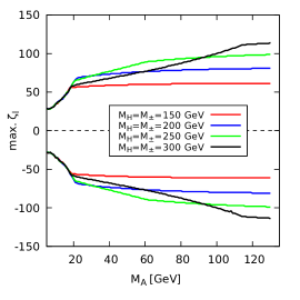
Figure 1: Maximum possible values of the lepton Yukawa parameter $\zeta_{l}$, given constraints from $\tau$- and $Z$-decays and collider data, as a function of $M_{A}$ for several values of $M_{H}=M_{H^{\pm}}$ as indicated.

The upper limits on $|\zeta_{l}|$ arise on the one hand from experimental constraints on the $\tau$-decay mode $\tau\to\mu\nu_{\tau}\bar{\nu}_{\mu}$ versus other decay modes and on leptonic $Z$-boson decays. 2HDM diagrams contributing to these decays involve tree-level or loop exchange of $A$ or $H^{\pm}$. They are enhanced by $\zeta_{l}$ and lead to disagreement with observations if $|\zeta_{l}|$ is too large. We computed the $\tau$- and $Z$-boson decays and the $\Delta\chi^{2}$ corresponding to the deviation from experiment as described in Ref. [23] and sec. 2.2.

On the other hand, further constraints on $\zeta_{l}$ arise from collider data. In particular, for small $M_{A}$ ($5<M_{A}<20$ GeV) the upper bound of $|\zeta_{l}|$ is dominated by the LEP process $ee\to\tau\tau(A)\to\tau\tau(\tau\tau)$ which was probed by the DELPHI collaboration [45]. In this decay, the electron positron pair annihilates into a $Z$-boson which further generates a pair of $\tau$-leptons. From one of those, a short-lived $A$ boson is created in resonance, producing finally two more taus.

Our resulting upper limits on $|\zeta_{l}|$ are shown in Fig. 1 as functions of $M_{A}$ for various choices of $M_{H^{\pm}}$. The limits are generally between $|\zeta_{l}|<40$ and $|\zeta_{l}|<100$. In most of the parameter space the limits are dominated by the $\tau$-decay constraints, which become weaker for larger $M_{A}$ and larger $M_{H},M_{H^{\pm}}$. The constraints from $Z$-boson decays become dominant for heavy Higgs masses above around 250 GeV. For even higher Higgs masses, these limits reduce the maximum $|\zeta_{l}|$ (see the black lines in Fig. 1). Aiming for largest possible Yukawa couplings, the $Z$-boson decay constraints imply that even larger heavy Higgs masses will not help. The constraints from LEP data are dominant for small $M_{A}<20$ GeV and significantly reduce the maximum $|\zeta_{l}|$ in this parameter region.

3.3 Constraints on the up-type Yukawa coupling $\zeta_{u}$

In this subsection we present the upper limits on $\zeta_{u}$, the parameter for up-type quark Yukawa couplings. This is a central part of our analysis, showing characteristic differences between the case of the type X model and the general flavour-aligned model. In what follows, we will focus on negative $\zeta_{l}$ (like in the type X model where $\zeta_{l}=-\tan\beta$) and positive $\zeta_{u}$, which leads to larger contributions to $a_{\mu}$.

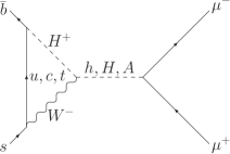
(a)

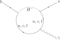
(b)

Figure 2: Sample Feynman diagrams for the processes $B_{s}\to\mu^{+}\mu^{-}$ and $b\to s\gamma$, which depend on the Yukawa couplings of up- and down-type quarks and leptons.

In type II or type X models $\zeta_{u}$ is always small for large lepton Yukawa coupling, because $\zeta_{u}=-1/\zeta_{l}=1/\tan\beta$. However, if general Yukawa couplings are allowed, $\zeta_{u}$ can be larger. The maximum possible value is interesting not only for $g-2$ but also in view of future LHC searches for a low-mass $A$.

We find that $\zeta_{u}$, in the scenario of $M_{A}<M_{h}$ and large $\zeta_{l}$, is constrained in a complementary way by B-physics on the one hand, and by LHC-data on the other hand.

Beginning with B-physics, the most constraining observables for this scenario are $b\to s\gamma$ and $B_{s}\to\mu^{+}\mu^{-}$. The sample diagrams shown in Fig. 2 illustrate that the 2HDM predictions depend on combinations of all Yukawa parameters $\zeta_{l}$, $\zeta_{u}$, $\zeta_{d}$ and on the Higgs masses $M_{A}$ and $M_{H^{\pm}}$. We have implemented the analytical results for the predictions presented in Refs. [46, 47] (Ref. [47] has also considered further observables, which however do not constrain the parameter space further; see also Ref. [48] for improvements on the precision of B-physics observables).

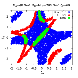
(a)

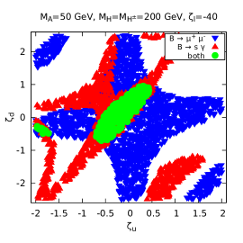
(b)

Figure 3: Allowed parameter regions in the $\zeta_{u}$–$\zeta_{d}$-plane given constraints from $b\to s\gamma$ or $B_{s}\to\mu^{+}\mu^{-}$ or the combination. The parameters are chosen as indicated.

To illustrate the interplay between the observables we show first Fig. 3. It shows the $2\sigma$ regions in the $\zeta_{u}$–$\zeta_{d}$-plane allowed by either $b\to s\gamma$ or $B_{s}\to\mu^{+}\mu^{-}$ alone or by the combination. In the figure, the representative values $M_{H^{\pm}}=200\text{ GeV, and }(M_{A},\zeta_{l})=(40\text{ GeV, }-60)\text{ or }(50\text{ GeV, }-40)$ are fixed, as indicated.

Both observables on their own would allow values of $\zeta_{u}\gg 1$, by fine-tuning $\zeta_{d}$ and $\zeta_{u}$. However, the combination of both observables implies an upper limit on $\zeta_{u}$, which in this case is $\zeta_{u}<0.5$.

By performing a similar analysis repeatedly, we obtain maximum values of $\zeta_{u}$ as function of $M_{A}$, $M_{H^{\pm}}$ and $\zeta_{l}$. The result will be shown below in the plots of Fig. 4 as continuous lines. Each solid line corresponds to the maximum allowed value (by B-physics) of $\zeta_{u}$, as a function of $M_{A}$ and for fixed values of $M_{H^{\pm}}$ and $\zeta_{l}$. The dependence on $M_{A}$, $M_{H^{\pm}}$ and $\zeta_{l}$ is mild. Generally, the upper limit on $\zeta_{u}$ is between $0.3$ and $0.6$.

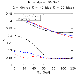
(a)

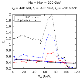
(b)

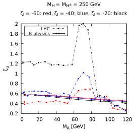
(c)

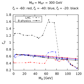
(d)

Figure 4: The maximum allowed values of $\zeta_{u}$ as function of $M_{A}$, for different values of $M_{H},M_{H^{\pm}}$ and $\zeta_{l}$ as indicated. The continuous lines correspond to the upper limit derived from B-physics alone, the dashed lines to the upper limit derived from LHC-Higgs physics alone.

Turning to LHC-Higgs physics, the dashed lines in the plots of Fig. 4 show the maximum $\zeta_{u}$ allowed by LHC collider constraints. These constraints on $\zeta_{u}$ arise from several processes and measurements:

• $pp\to A\to\tau\tau$ for $M_{A}>M_{Z}$ [49]. In our scenario $A$ decays essentially to $100\%$ into $\tau\tau$. Hence the measurement constrains the production rate of $A$, which proceeds via top-quark loop and gluon fusion and is thus governed by $\zeta_{u}$. Hence this measurement provides an essentially universal upper limit of approximately $\zeta_{u}<0.2$ which becomes valid above $M_{A}>100$ GeV.

• $pp\to H\to\tau\tau$ [49] if $H\to AA$ is kinematically forbidden. Similar to the previous case, $H$ is produced in gluon fusion via a top-loop, so its production rate is governed by $\zeta_{u}$; it decays essentially always into a $\tau$-pair. Hence, again, this measurement places an essentially universal upper limit on $\zeta_{u}$, valid if $M_{A}>M_{H}/2$. In the plots, this limit can be seen for $M_{H}=150$ GeV and $M_{A}>75$ GeV.

• $pp\to H\to\tau\tau$ [49] if $H\to AA$ is kinematically allowed. This case is relevant in the largest region of parameter space, including the regions with the peak structures in which the collider limits become rather weak and $\zeta_{l}$-dependent. The scalar Higgs $H$ is produced in gluon fusion via a top-loop, so its production rate is governed by $\zeta_{u}$; its two most important decay modes are $H\to AA$ and $H\to\tau\tau$. Hence, the signal strength for the full process depends not only on $\zeta_{u}$ but also on the triple Higgs coupling $C_{HAA}$, which is strongly correlated with $C_{HH^{+}H^{-}}$ given in Eq. (20). The signal strength can be suppressed by small $\zeta_{u}$ (which suppresses the production) or by large $C_{HH^{+}H^{-}}$ (which suppresses the decay to $\tau\tau$).

  Hence we show the allowed ranges of $\zeta_{u}$ and the triple Higgs coupling $C_{HH^{+}H^{-}}$ in Fig. 5, for the representative values $M_{A}=50/80$ GeV, $M_{H}=M_{H^{\pm}}=200$ GeV, $\zeta_{l}=-40$. The colours indicate the successive application of constraints from the electroweak S, T, U parameters, HiggsBounds, HiggsSignals, and tree-level stability, unitarity and perturbativity (as implemented in 2HDMC [39]). The border of the yellow region shows clearly the correlation between the two couplings mentioned above, needed to evade the constraints from $pp\to H\to\tau\tau$ searches. The larger the triple Higgs coupling, the larger $\zeta_{u}$ can be. However, perturbativity restricts the triple Higgs coupling, and this restriction depends on whether $M_{A}<M_{h}/2$ holds or not. If $M_{A}<M_{h}/2$, the relation (12) following from setting to zero Eq. (A) has to be used, and the maximum triple Higgs coupling and thus the maximum $\zeta_{u}$ is smaller.

  As a result of this combination of constraints, the LHC-Higgs limits on $\zeta_{u}$ are rather loose for $M_{A}$ between $M_{h}/2$ and around $M_{Z}$ (explaining the peaks in Fig. 4), and stronger for lower $M_{A}$. The precise value of the limits depends on $\zeta_{l}$, which also influences the branching ratio $H\to\tau\tau$.

• We also mention the analysis of Ref. [27], where LHC-constraints on the type X model have been studied; since $\zeta_{u}$ is negligible in the type X model, those constraints are weaker than the ones we consider here, and they do not limit $\zeta_{u}$. Still, that analysis shows that data from multi-Higgs production followed by decays into multi-$\tau$ final states leads to interesting (mild) constraints on heavy $M_{H}$, $M_{H^{\pm}}$.

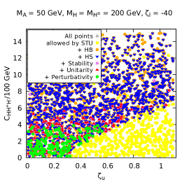
(a)

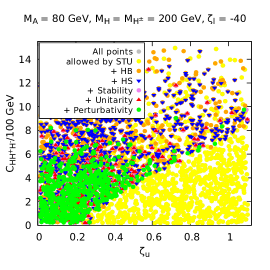
(b)

Figure 5: Allowed ranges of $\zeta_{u}$ and the triple Higgs coupling $C_{HH^{+}H^{-}}$, given certain constraints, see legend and text. The constraints are applied successively. The scanned parameter space is defined by Eq. (7), with Eq. (12) in case $M_{A}<M_{h}/2$.

4 Bosonic contributions to $a_{\mu}$ and relevant parameter constraints

As discussed in the previous section, the 2HDM parameter region of interest for $a_{\mu}$ is characterized by large Yukawa coupling parameter $\zeta_{l}$ and small pseudoscalar mass $M_{A}$. The bosonic two-loop contributions $a_{\mu}^{\text{B}}$ computed in Ref. [30] depend on a large number of additional parameters: the physical Higgs masses $M_{H}$, $M_{H^{\pm}}$, the mixing angle $c_{\beta\alpha}$, $\tan\beta$, and the Higgs potential parameters $\lambda_{1}$ and $\lambda_{6,7}$. In the present section we provide an overview of the influence of these parameters, constraints on their values, and update the analysis of Ref. [30] given those constraints. As a result we derive the maximum possible values of the bosonic two-loop contributions to $a_{\mu}$.

The bosonic two-loop contributions can be split into three parts [30],

$$a_{\mu}^{\text{B}} =a_{\mu}^{\text{EW add.}}+a_{\mu}^{\text{non-Yuk}}+a_{\mu}^{\text{Yuk}},$$ (13)

where $a_{\mu}^{\text{EW add.}}$ denotes the difference between the contribution of the SM-like Higgs in the 2HDM and its SM counterpart; $a_{\mu}^{\text{non-Yuk}}$ and $a_{\mu}^{\text{Yuk}}$ denote remaining bosonic contributions without/with Yukawa couplings.

We begin with a discussion of $a_{\mu}^{\text{EW add.}}$, which is approximately given by $a_{\mu}^{\text{EW add.}}=2.3\times 10^{-11}\,c_{\beta\alpha}\,\zeta_{l}$. As discussed in section 3.1, the product $c_{\beta\alpha}\,\zeta_{l}$ is restricted by Higgs signal strength measurements to be smaller than unity. Hence this product can never be an enhancement factor. Specifically, as a result we obtain the conservative limit

$$|a_{\mu}^{\text{EW add.}}| <0.2\times 10^{-10}\,,$$ (14)

such that these contributions are negligible.

Next we consider $a_{\mu}^{\text{non-Yuk}}$, the contribution from diagrams in which the extra 2HDM Higgs bosons couple only to SM gauge bosons and not to fermions. Similar to the quantity $\Delta\rho$, this contribution is enhanced by large mass splittings $|M_{H}-M_{H^{\pm}}|$ between the heavy Higgs bosons. Conversely, constraints on $\Delta\rho$ restrict this mass splitting [22, 50] and thus $a_{\mu}^{\text{non-Yuk}}$. We find that $a_{\mu}^{\text{non-Yuk}}$ is similarly negligible as Eq. (14).

Finally we turn to $a_{\mu}^{\text{Yuk}}$, the potentially largest bosonic two-loop contribution. Ref. [30] has decomposed this contribution into several further subcontributions depending on the appearance of triple Higgs couplings, the mixing angle $c_{\beta\alpha}$ and the Yukawa parameter $\zeta_{l}$. Among these parameters, the product $c_{\beta\alpha}\,\zeta_{l}$ is restricted as discussed above; furthermore, the triple Higgs couplings are constrained by perturbativity. Inspection of the results of Figs. 5 and 6 of Ref. [30] then shows that all subcontributions to $a_{\mu}^{\text{Yuk}}$ are at most of the order $10^{-11}$, with the exception of the ones enhanced by the triple Higgs coupling $C_{HH^{+}H^{-}}$.

Hence the overall bosonic two-loop contributions are essentially proportional to the value of the coupling $C_{HH^{+}H^{-}}$. Likewise, all the parameters $\tan\beta$, $\lambda_{1,6,7}$ enter the prediction for $a_{\mu}$ essentially via this coupling. This proportionality is shown in Fig. 6(a), which displays the ratio $\rho$, defined via

$$|a_{\mu}^{\text{B}}| =\rho|C_{HH^{+}H^{-}}/\text{GeV}|\,|\zeta_{l}|\times 10^{-15}$$ (15)

as a function of $a_{\mu}^{\text{B}}$ in a scan of parameter space. The approximate proportionality clearly emerges, if $a_{\mu}^{\text{B}}$ is larger than around $0.5\times 10^{-10}$. The quantity $\rho$ then only depends on the heavy Higgs masses, and its value is $\rho\approx 6,3,2,1$ (for $M_{H}=M_{H^{\pm}}=150,200,250,300$ GeV, respectively). In Fig. 6(a) we display only positive $a_{\mu}^{\text{B}}$. The sign of $a_{\mu}^{\text{B}}$ also depends on the triple Higgs coupling (see the explicit formula in the appendix). For small $c_{\beta\alpha}$ it is thus determined essentially by $(\tan\beta-1)$. If $\tan\beta<1$, $a_{\mu}^{\text{B}}$ is positive (for negative $\zeta_{l}$ and with small corrections if $c_{\beta\alpha}\neq 0$).

Hence we mainly need to discuss the behaviour of the coupling $C_{HH^{+}H^{-}}$. We need to distinguish two cases:

• 2HDM type I, II, X, Y: here $\tan\beta$ and the Yukawa parameters are correlated. Specifically in the most interesting case of the type X model, $\tan\beta=-\zeta_{l}$ and is therefore large. As a result, the triple Higgs coupling is suppressed, and the overall bosonic contribution $a_{\mu}^{\text{B}}$ is negligible.

• General aligned 2HDM: in this case $\tan\beta$ is independent of $\zeta_{l}$, and the triple Higgs coupling $C_{HH^{+}H^{-}}$ can be largest if $\tan\beta={\cal O}(1)$.

Focusing now on the second case of the aligned 2HDM, the range of possible values of $C_{HH^{+}H^{-}}$ can already be seen in Fig. 5 for particular choices of $M_{A}=50/80$ GeV, $M_{H}=M_{H^{\pm}}=200$ GeV, $\zeta_{l}=-40$. There, large $C_{HH^{+}H^{-}}$ was important to suppress the branching ratio of $H\to\tau\tau$ and allow large values for $\zeta_{u}$. For $M_{A}=80$ GeV all parameters $\lambda_{1,6,7}$ and $\tan\beta$ have been varied in the full range of Eq. (7), and the maximum allowed triple Higgs coupling is around $1000$ GeV. For $M_{A}=50$ GeV, on the other hand, $\lambda_{1}$ is fixed as explained in sec. 3.1 to suppress the decay $h\to AA$. Hence the maximum triple Higgs coupling is smaller, in this case around 400 GeV.

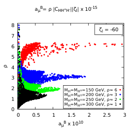
(a)

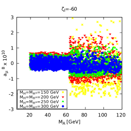
(b)

Figure 6: The bosonic contributions $a_{\mu}^{\text{B}}$. (a) The proportionality factor $\rho$ defined in Eq. (15) for a scan of parameter space with different values of the heavy Higgs masses. (b) The range of possible values for $a_{\mu}^{\text{B}}$. The scanned parameter space is defined by Eq. (7), with Eq. (12) in case $M_{A}<M_{h}/2$. Only points passing all constraints of sec. 3 are shown. Plot (a) would remain essentially the same for other choices of $\zeta_{l}$, and plot (b) would change essentially linearly with $\zeta_{l}$. In plot (b), part of the region below $M_{A}<20$ GeV is excluded for $\zeta_{l}=-60$, corresponding to the limit in Fig. 1.

The results generalize to other values of $M_{A}$. The maximum triple Higgs coupling essentially only depends on whether $M_{A}$ is smaller or larger than $M_{h}/2$. In the latter case, the triple Higgs coupling reaches around $1000$ GeV, in the former case only around $400\ldots 600$ GeV, depending on the heavy Higgs masses $M_{H}$, $M_{H^{\pm}}$.

Figure 6(b) shows the range of possible bosonic contributions $a_{\mu}^{\text{B}}$ as a function of $M_{A}$ for various values of $M_{H}=M_{H^{\pm}}$. The result is fully understood with the proportionality (15) and the maximum values for $C_{HH^{+}H^{-}}$ just discussed. We display the result only for a particular value of $\zeta_{l}$ but we have checked that the results are exactly linear in $\zeta_{l}$ as expected. We have also checked that the maximum results do not change significantly if the heavy Higgs masses are varied independently, $M_{H}\neq M_{H^{\pm}}$, or if $\lambda_{6,7}$ are set to zero.

As a result of the analysis of the individual contributions to $a_{\mu}^{\text{B}}$ and of $C_{HH^{+}H^{-}}$ we can now summarize the maximum possible $a_{\mu}^{\text{B}}$ in the simple approximation formula

$$|a_{\mu}^{\text{B}}|^{\text{max}} \approx\left\{\begin{array}[]{c}1\\ 0.5\end{array}\right\}\,\rho\,|\zeta_{l}|\times 10^{-12}$$ (18)

where the upper (lower) result holds for $M_{A}>M_{h}/2$ $(<M_{h}/2)$ and where $\rho=6,3,2,1$ for $M_{H}=M_{H^{\pm}}=150,200,250,300$ GeV, respectively.

5 Muon $g-2$ in the 2HDM

In this section we use the previous results on limits on relevant parameters to discuss in detail the possible values of $a_{\mu}$ in the 2HDM, answering the two questions raised in the introduction. Subsection 5.1 discusses $a_{\mu}$ as a function of the relevant parameters and characterizes parameter regions giving particular values for $a_{\mu}$; subsection 5.2 provides the maximum $a_{\mu}$ that can be obtained in the 2HDM overall or for certain parameter values.

Before entering details, we provide here useful approximation formulas for $a_{\mu}$ in the 2HDM, which provide the correct qualitative behaviour in the parameter region of interest with small $M_{A}$ and large lepton Yukawa coupling $\zeta_{l}$. The one-loop contributions $a_{\mu}^{{\text{2HDM}},1}$ are dominated by diagrams with $A$ exchange; the fermionic two-loop contributions $a_{\mu}^{\text{F}}$ are dominated by diagrams with $\tau$-loop and $A$ exchange or top-loop and $A,H,H^{\pm}$ exchange; the bosonic two-loop contributions $a_{\mu}^{\text{B}}$ are dominated by diagrams with $H$ exchange and $H^{\pm}$-loop. The numerical approximations for these contributions are, using $\hat{x}_{\cal S}\equiv{M_{\cal S}}/{100\;\text{GeV}}$ and $M_{H^{\pm}}=M_{H}$,

$$a_{\mu}^{{\text{2HDM}},1} \simeq\Big{(}\frac{\zeta_{l}}{100}\Big{)}^{2}\,\Big{\{}\frac{-3-0.5\ln(\hat{x}_{A})}{\hat{x}_{A}^{2}}\Big{\}}\,\times 10^{-10}\,,$$ (19a)

$$a_{\mu}^{\text{F}}{}^{\tau} \simeq\left(\frac{\zeta_{l}}{100}\right)^{2}\,\Big{\{}\frac{8+4\hat{x}_{A}^{2}+2\ln(\hat{x}_{A})}{\hat{x}_{A}^{2}}\Big{\}}\,\times 10^{-10}\,,$$ (19b)

$$a_{\mu}^{\text{F}}{}^{t} \simeq\left(\frac{-\zeta_{l}\zeta_{u}}{100}\right)\,\Big{\{}22-14\ln(\hat{x}_{A})+32-15\ln(\hat{x}_{H})\Big{\}}\,\times 10^{-10}\,,$$ (19c)

$$|a_{\mu}^{\text{B}}| \simeq\rho|C_{HH^{+}H^{-}}/\text{GeV}|\,|\zeta_{l}|\times 10^{-15}\,.$$ (19d)

The sign of the $\tau$-loop contribution is positive in our parameter region; the one-loop contributions are negative but are subdominant except at very small $M_{A}$. The top-loop contribution is positive if $\zeta_{u}$ has a sign opposite to $\zeta_{l}$, which is why we choose $\zeta_{l}<0$ and focus on $\zeta_{u}>0$. $a_{\mu}^{\text{B}}$ is positive if $\zeta_{l}<0$ and $\tan\beta<1$ (up to small corrections if $a_{\mu}^{\text{B}}$ is small); see sec. 4 for further details on the quantity $\rho$ and the approximation for $a_{\mu}^{\text{B}}$.

For the exact results we refer to the literature. The full two-loop result has been obtained and documented in Ref. [30]; the full set of Barr-Zee diagrams has been obtained in Ref. [29]; for earlier results we refer to the references therein. In our numerical evaluation we use the results of Ref. [30].

5.1 $a_{\mu}$ in different parameter regions

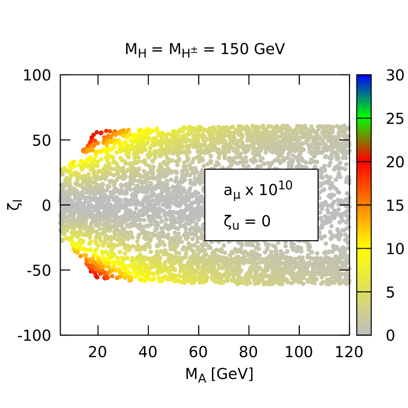
(a)

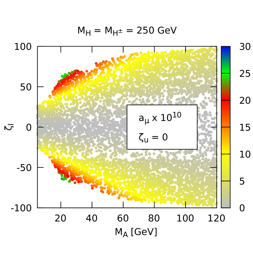
(b)

Figure 7: $a_{\mu}$ in the 2HDM (from two-loop fermionic and one-loop contributions, and in units of $10^{-10}$), as a function of $M_{A}$ and the $\tau$-Yukawa parameter $\zeta_{l}$; the current deviation (1) corresponds to green points. Only points in the allowed region of Fig. 1 are shown. The parameter $\zeta_{u}$ is set to zero, corresponding to the case with vanishing top-loop contributions and approximately to the type X model case. The parameters $M_{H}$, $M_{H^{\pm}}$ are fixed as indicated. Corresponding plots with $M_{H},M_{H^{\pm}}=200,300$ GeV would look very similar, except for the slightly different allowed regions.

Here we discuss the question raised in the introduction: In which parameter region can the 2HDM accommodate the current deviation in $a_{\mu}$ (or a future, possibly larger or smaller deviation)?

We begin by listing several remarks which can be obtained from the results of the previous sections.

• All important contributions to $a_{\mu}$ are proportional to the lepton Yukawa coupling parameter $\zeta_{l}$ or $\zeta_{l}^{2}$ (where e.g. in the type X model $\zeta_{l}=-\tan\beta$). Hence $\zeta_{l}$ must be much larger than unity in order to obtain significant $a_{\mu}$. From section 3.3 we then obtain that the quark Yukawa parameters $\zeta_{u}$, $\zeta_{d}$ can be at most of order unity.

  This implies that the bottom loop contribution is negligible, and that the type X model is the only of the usual four discrete symmetry models with significant $a_{\mu}$ (see also Ref. [22]).

• The single most important contribution to $a_{\mu}$ is the one from the $\tau$-loop, see Eq. (19). It depends on $\zeta_{l}$ and $M_{A}$. In the general flavour-aligned model, the top-loop contribution can also be significant provided $\zeta_{u}$ is close to its maximum value of order unity.

• The masses of the heavy Higgs bosons $H$ and $H^{\pm}$ are relatively unimportant for $a_{\mu}$. However, they are important for the limits on the possible values of $\zeta_{l}$ and $\zeta_{u}$. If these Higgs bosons have masses around 250 GeV the largest $|\zeta_{l}|$ up to 100 are allowed in most of the parameter space. For even higher masses the limits on $|\zeta_{l}|$ become slightly stronger and the limits on $\zeta_{u}$ saturate thanks to Z-decay and LHC search limits.

• The mass splitting between $M_{H}$ and $M_{H^{\pm}}$ is unimportant. It is strongly restricted by limits from electroweak precision observables [22, 50] and we have checked that its remaining influence on the limits on $\zeta_{l}$, $\zeta_{u}$ and on the bosonic contributions $a_{\mu}^{\text{B}}$ is negligible. Hence we set $M_{H}=M_{H^{\pm}}$ in all our numerical examples.

• The Higgs mixing angle $c_{\beta\alpha}$ is unimportant for $a_{\mu}$. For our scenario of interest it is mostly limited by LHC measurements of Higgs couplings to leptons, which restrict $|c_{\beta\alpha}\zeta_{l}|$ to be smaller than order one. Hence all contributions to $a_{\mu}$ depending on $c_{\beta\alpha}$ are strongly suppressed.

• The parameters $\lambda_{1,6,7}$ and $\tan\beta$ from the Higgs potential appear in $a_{\mu}$ essentially only via the triple Higgs coupling $C_{HH^{+}H^{-}}$, which in turn is maximized for $\tan\beta={\cal O}(1)$. In the type X model with large $\tan\beta=-\zeta_{l}$ this strongly suppresses the bosonic contributions $a_{\mu}^{\text{B}}$; in the more general aligned model, the bosonic diagrams behave as given in Eq. (19d).

  In the plots of this subsection we do not include the bosonic contributions $a_{\mu}^{\text{B}}$ because their parameter dependence is clear from this discussion, because their sign can be positive or negative, and because their numerical impact is small.

Figures 7 and 8 show $a_{\mu}$ as a function of the most important parameters $M_{A}$, $\zeta_{l}$ and $\zeta_{u}$ and the heavy Higgs masses $M_{H},M_{H^{\pm}}$.

Fig. 7 focuses on the two most important parameters $M_{A}$ and the lepton Yukawa coupling $\zeta_{l}$. It shows $a_{\mu}$ (including one-loop and fermionic two-loop contributions) as a function of $M_{A}$ and $\zeta_{l}$. The top-Yukawa parameter $\zeta_{u}$ is fixed to $\zeta_{u}=0$; hence only the $\tau$-loop and the one-loop contributions are significant. The result also corresponds to the type X model, in which $\zeta_{u}$ is negligible. We further fix $M_{H}=M_{H^{\pm}}=150,250$ GeV and show only parameter points allowed by the constraints of sec. 3.2. The results for $a_{\mu}$ are not very sensitive to the choice of $M_{H},M_{H^{\pm}}$, but for $M_{H}=M_{H^{\pm}}=250$ GeV the allowed parameter space is largest.

Even at the border of the allowed region, a contribution as large as the deviation (1) can barely be obtained (see also the discussions in Refs. [25, 23]). Only in the small corner with $M_{A}\sim 20$ GeV and $|\zeta_{l}|\sim 70$, $a_{\mu}$ comes close to explaining Eq. (1). More generally, the plot reflects the behaviour that $a_{\mu}$ is dominated by the $\tau$-loop which in turn is approximately proportional to $(\zeta_{l}/M_{A})^{2}$. A contribution above approximately $20$ (in units of $10^{-10}$) is possible in the small region where $|\zeta_{l}/M_{A}|>2\text{GeV}^{-1}$, which is allowed for around $M_{A}\sim 20\ldots 40$ GeV. Even smaller contributions above $10$ are difficult to obtain. They require $|\zeta_{l}/M_{A}|>1\text{GeV}^{-1}$ and are possible for $M_{A}$ up to around $60\ldots 80$ GeV.

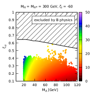
(a)

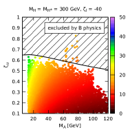
(b)

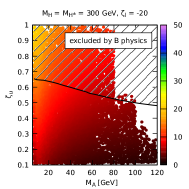
(c)

Figure 8: $a_{\mu}$ in the 2HDM (from two-loop fermionic and one-loop contributions, and in units of $10^{-10}$), as a function of $M_{A}$ and the top-Yukawa parameter $\zeta_{u}$; the current deviation (1) corresponds to yellow/green points. Only points allowed by the collider constraints of Fig. 4 are shown; the B-physics constraints are shown as the hatched regions. The parameters $\zeta_{l}$ and $M_{H}$, $M_{H^{\pm}}$ are fixed as indicated. Corresponding plots with other choices of $M_{H}$, $M_{H^{\pm}}$ would look very similar, except for the different allowed parameter regions.

The impact of the top-loop for $\zeta_{u}\neq 0$ can be seen in Fig. 8. It shows $a_{\mu}$ (including one-loop and fermionic two-loop contributions) as a function of $M_{A}$ and $\zeta_{u}$. In the plot, $\zeta_{l}$ is fixed to exemplary values $\zeta_{l}=-20,-40,-60$. Because of the sum of $\tau$- and top-loops the dependence on $\zeta_{l}$ is non-linear, and the relative importance of the top-loop and thus of the parameter $\zeta_{u}$ is higher for smaller $\zeta_{l}$.

We display $a_{\mu}$ for all points which pass the collider constraints discussed in sec. 3.3, and we display the constraints from B-physics on the maximum $\zeta_{u}$ as a line in the plots. In Fig. 8 we do not show all choices of the heavy Higgs masses $M_{H},M_{H^{\pm}}$ but fix $M_{H}=M_{H^{\pm}}=300$ GeV. Like in the previous figure, the values of $a_{\mu}$ would be essentially independent of the heavy Higgs masses; the behaviour of the collider and B-physics constraints can be obtained from Fig. 4.

Nonzero $\zeta_{u}$ helps in explaining the current $a_{\mu}$ deviation (1) of around $30$ (in units of $10^{-10}$). The fan-shaped structure of the plots shows that higher values of the Higgs mass $M_{A}$ can be compensated by larger $\zeta_{u}$ to obtain the same $a_{\mu}$. For instance, for $\zeta_{l}=-60$, contributions to $a_{\mu}$ around $30$ can be obtained up to $M_{A}\sim 40$ GeV. Contributions above $20$ can be obtained up to $M_{A}\sim M_{Z}$, by taking advantage of the larger allowed values of $\zeta_{u}$ in this mass range.

For smaller $\zeta_{l}=-40$, contributions above $20$ are possible for $M_{A}$ up to around $60$ GeV, and contributions above $10$ are possible up to $A\sim M_{Z}$. For $\zeta_{l}=-20$, the contributions to $a_{\mu}$ are generally smaller than $20\times 10^{-10}$, but even here nonzero $\zeta_{u}$ strongly increases $a_{\mu}$.

5.2 Maximum possible $a_{\mu}$ in the 2HDM

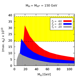
(a)

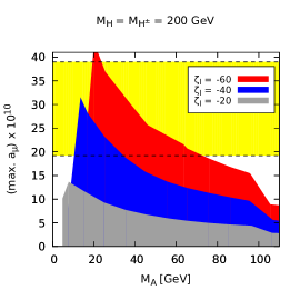
(b)

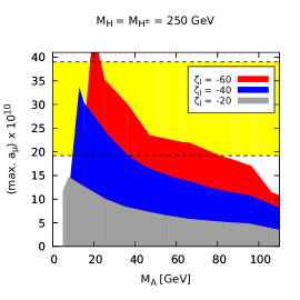
(c)

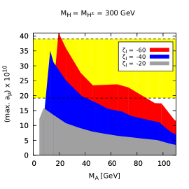
(d)

Figure 9: The maximum $a_{\mu}$ (including one-loop and all two-loop contributions) for several fixed values of $\zeta_{l}$ and $M_{H}=M_{H^{\pm}}$. For each $M_{A}$ and $\zeta_{l}$, the maximum $\zeta_{u}$ is obtained from the results of sec. 3.3. The yellow band indicates the current $a_{\mu}$ deviation, defined by taking the envelope of the $1\sigma$ bands given by Eq. (1).

Now we discuss the question: What is the overall maximum possible value of $a_{\mu}$ that can be obtained in the 2HDM? Fig. 9 and 10 show the maximum possible $a_{\mu}$ in the 2HDM, first for fixed choices of the lepton Yukawa coupling $\zeta_{l}=-20,-40,-60$, then overall.

Fig. 9 is obtained by maximizing $\zeta_{u}$ for each parameter point, given all constraints discussed in sec. 3.3. The plots clearly show the prominent role of $M_{A}$ and the lepton Yukawa coupling $\zeta_{l}$. The values of the heavy Higgs bosons $M_{H},M_{H^{\pm}}$ mainly matter because they influence the maximum allowed value of $\zeta_{u}$. Only two cases need to be clearly distinguished: small $M_{H},M_{H^{\pm}}=150$ GeV and larger $M_{H},M_{H^{\pm}}=200,250,300$ GeV, which all lead to similar results for $a_{\mu}$.

For each value of $\zeta_{l}$, there is a sharp maximum around $M_{A}\sim 20$ GeV. At the maximum, $a_{\mu}$ obviously depends on $\zeta_{l}$, but also on the heavy Higgs masses $M_{H},M_{H^{\pm}}$, because their values influence the maximum allowed value of $\zeta_{u}$. For $\zeta_{l}=-60(-40)$ and large $M_{H},M_{H^{\pm}}$, $a_{\mu}$ reaches $40(30)\times 10^{-10}$, which is larger than the currently observed deviation (1). For $M_{H}=M_{H^{\pm}}=150$ GeV or $\zeta_{l}=-20$, the contributions to $a_{\mu}$ are smaller.

For values of $M_{A}$ lower than at the peaks in Fig. 9, the maximum $a_{\mu}$ values drop sharply (the drop is at lower $M_{A}$ if $\zeta_{l}$ is smaller). The reason is that for each $\zeta_{l}$ there is a minimum allowed value of $M_{A}$ mainly because of the collider limits discussed in sec. 3.2. Even if lower values of $M_{A}$ were allowed, $a_{\mu}$ would be suppressed by the negative one-loop contribution.

For higher values of $M_{A}$, $a_{\mu}$ is suppressed by $M_{A}$. As can be estimated from the approximation (19), the suppression is weaker than $1/M_{A}^{2}$. Further the suppression is modulated by the maximum possible value of $\zeta_{u}$. In particular, above $M_{A}>M_{h}/2$, higher values of $\zeta_{u}$ are allowed, and the maximum $a_{\mu}$ drops more slowly with $M_{A}$.

In summary, the deviation (1) can be explained at the $1\sigma$ level for $M_{A}=20\ldots 40$ GeV and for $\zeta_{l}=-40$ and high $M_{H},M_{H^{\pm}}$ or $\zeta_{l}=-60$ independently of $M_{H},M_{H^{\pm}}$. It can further be explained for $M_{A}=20\ldots 80$ GeV for $\zeta_{l}=-60$ if $M_{H},M_{H^{\pm}}$ are high.

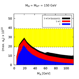
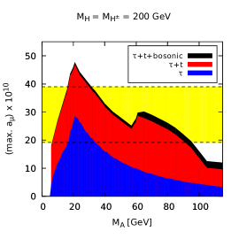
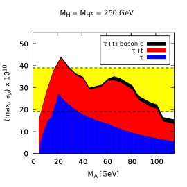
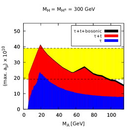
Figure 10: The overall maximum $a_{\mu}$ (including one-loop and all two-loop contributions) as a function of $M_{A}$, for several fixed values of $M_{H}=M_{H^{\pm}}$. For each value of $M_{A}$, the maximum value of $|\zeta_{l}|$ is determined as in sec. 3.2; then the maximum $\zeta_{u}$ is obtained from the results of sec. 3.3. The result without top-loop and bosonic contributions (which would correspond to the maximum in the type X model) is shown in blue; the result without bosonic two-loop contributions in red; the total maximum result, including the maximum bosonic contributions in black. The yellow band indicates the current $a_{\mu}$ deviation, defined by taking the envelope of the $1\sigma$ bands given by Eq. (1).

The overall maximum $a_{\mu}$ in the flavour-aligned 2HDM can be seen in Fig. 10 for several choices of $M_{H},M_{H^{\pm}}$. The figure is obtained by maximizing first $\zeta_{l}$ (i.e. the $\tau$-loop contribution), then $\zeta_{u}$ (i.e. the top-loop contribution), and finally the bosonic two-loop contribution for each parameter point. All constraints discussed in secs. 3.2, 3.3 are employed.

The plots display not only the final total result for $a_{\mu}$ including all one- and two-loop contributions. They also display the results of the $\tau$-loop (plus one-loop) contribution alone, and the results including the top-loop but excluding the bosonic two-loop contributions. In this way the plots allow to read off the results corresponding to the 2HDM type X, and to read off the influence of the bosonic two-loop corrections.

Starting the discussion with the type X model result (blue), the plots confirm that the type X model can barely explain the current deviation (1). The largest values that can be obtained are around $27\times 10^{-10}$ at $M_{A}=20$ GeV for $M_{H},M_{H^{\pm}}=200\ldots 250$ GeV. For higher or lower values of $M_{A}$ the maximum type X contributions drop quickly, and values above $20\times 10^{-10}$ can only be obtained between $M_{A}=20\ldots 40$ GeV.

Hence going beyond the type X model and allowing general Yukawa couplings significantly widens the parameter space which can lead to significant contributions to $a_{\mu}$. Both the top-loop and the bosonic two-loop contributions can significantly increase $a_{\mu}$. Thanks to the behaviour discussed in sec. 4 and expressed in Eqs. (19) both of these contributions are not significantly suppressed by heavier $M_{A}$. On the contrary, for heavier $M_{A}$, larger $\zeta_{u}$ and larger triple Higgs couplings $C_{HH^{+}H^{-}}$ are allowed, and the loop functions are not strongly suppressed by heavy $M_{A}$.

Thus, in the general (flavour-)aligned 2HDM one can obtain even $a_{\mu}>45\times 10^{-10}$ if $M_{A}\sim 20$ GeV and if $M_{H},M_{H^{\pm}}$ are in the range 200…250 GeV. Hence the 2HDM could even accommodate a larger deviation than (1), which might be established at forthcoming $a_{\mu}$ measurements. Thanks to the large possible values of the top Yukawa parameter $\zeta_{u}$, the current deviation can be explained at the $1\sigma$ level in all the range $M_{A}=20\ldots 100$ GeV.

6 Summary and conclusions

The 2HDM is a potential source of significant contributions to the anomalous magnetic moment of the muon $a_{\mu}$, and it could explain the current deviation (1). Here we have provided a comprehensive analysis of the relevant parameter space and of possible flavour-aligned 2HDM contributions to $a_{\mu}$. Our analysis was kept general, anticipating that future $a_{\mu}$ measurements might further increase or decrease the deviation (1).

The relevant parameter space is characterized by light pseudoscalar Higgs with mass $M_{A}<100$ GeV and large Yukawa couplings to leptons. Among the usual 2HDM models with discrete symmetries this is only possible in the lepton-specific type X model. In the type X model, large lepton Yukawa couplings imply negligible quark Yukawa couplings to the $A$ boson. We considered the more general flavour-aligned model, which contains type X as a special case but in which simultaneously significant Yukawa couplings to quarks are possible.

We first investigated the allowed values of the Yukawa coupling parameters $\zeta_{l}$ and $\zeta_{u,d}$ (which would be given by $-\tan\beta$ and $1/\tan\beta$ in the type X model). An extensive summary of the results is provided at the beginning of sec. 5.1. In short, the lepton Yukawa coupling $|\zeta_{l}|$ can take values up to $40\ldots 100$, depending on the values of all Higgs masses. For very light $M_{A}<20$ GeV, very severe limits from LEP data reduce the maximum $|\zeta_{l}|$ and thus the maximum $a_{\mu}$. For large lepton Yukawa coupling, both quark Yukawa couplings $\zeta_{u,d}$ can be ${\cal O}(0.5)$ at most because of B-physics data and LHC-Higgs searches. While $\zeta_{d}$ has negligible influence on $a_{\mu}$, in particular the upper limit on the top Yukawa coupling $\zeta_{u}$ is critical for $a_{\mu}$. Interestingly, for $M_{A}>M_{h}/2$ GeV, slightly larger values of $\zeta_{u}$ are allowed thanks to an interplay between the triple Higgs couplings and the Yukawa coupling.

As an intermediate result and an update of the results of Ref. [30] on the full two-loop calculation of $a_{\mu}$ in the 2HDM, we evaluated the maximum contributions $a_{\mu}^{\text{B}}$ from bosonic two-loop diagrams. Going beyond the type X model can also increase $a_{\mu}^{\text{B}}$. The maximum is mainly determined by the maximum triple Higgs coupling, which is obtained if $\tan\beta\ll|\zeta_{l}|$. It reaches $3\times 10^{-10}$ if $\zeta_{l}$ is also maximized and if $M_{A}$ is around 100 GeV and the heavy Higgs masses $M_{H},M_{H^{\pm}}$ are not much higher.

Figures 7,8,9,10 answer the questions how $a_{\mu}$ depends on the 2HDM parameters, and what is the maximum $a_{\mu}$ that can be obtained in the 2HDM. The overall maximum is above $45\times 10^{-10}$, and it can be obtained for $M_{A}\sim 20$ GeV. More generally contributions significantly above the current deviation (1) can be obtained for $M_{A}$ up to $40$ GeV. Thanks to the large allowed top Yukawa coupling, the current deviation (1) can be explained at the $1\sigma$ level for $M_{A}$ up to 100 GeV. Even if the lepton Yukawa coupling is not maximized but fixed at only $\zeta_{l}=-40$, a $1\sigma$ explanation is possible up to $M_{A}=40$ GeV. The heavy Higgs masses $M_{H}$ and $M_{H^{\pm}}$ are not very critical; the maximum $a_{\mu}$ is obtained if they are in the range 200…300 GeV; for lower or higher masses the limits on the Yukawa couplings become stronger, and significantly higher masses are disfavoured by triviality constraints [22, 25].

For the type X model, the maximum contributions are significantly smaller, only slightly above $25\times 10^{-10}$. A $1\sigma$ explanation of the current deviation is only possible in the small range of $M_{A}$ between 20 and 40 GeV, and even a potential future deviation of only $10\times 10^{-10}$ can be explained only for $M_{A}<80$ GeV.

In view of these results it is of high interest to test this parameter space more fully at the LHC. In view of the significant couplings of the low-mass $A$ boson to $\tau$ leptons and top quarks, it is promising to derive more stringent upper limits on these couplings, particularly on the product $|\zeta_{l}\zeta_{u}|$. Such more stringent limits will have immediate impact on the possible values of $a_{\mu}$ in the 2HDM. At the same time, the future $a_{\mu}$ measurements have a high potential to constrain the 2HDM parameter space. In particular the type X model might be excluded by a confirmation of a large $a_{\mu}$ deviation, and in the more general model, lower limits on the top Yukawa coupling and upper limits on $M_{A}$ might be derived.

Appendix A Explicit results for triple Higgs couplings

Here we provide the explicit results for the triple Higgs couplings which are required for our analysis. The triple Higgs couplings of the heavy Higgs $H$ to either $AA$ or $H^{\pm}H^{\mp}$ are correlated as

$$C_{HH^{+}H^{-}}= C_{HAA}-2\left(\frac{M_{H^{\pm}}^{2}-M_{A}^{2}}{v}\right)c_{\beta\alpha}\,,$$ (20)

and $C_{HAA}$ is given by

$$C_{HAA}= \lambda_{1}v\Big{(}s_{\beta\alpha}\frac{1-t_{\beta}^{2}}{t_{\beta}^{3}}-c_{\beta\alpha}\frac{2}{t_{\beta}^{2}}\Big{)}+s_{\beta\alpha}\frac{M_{h}^{2}}{v}\frac{t_{\beta}^{2}-1}{t_{\beta}^{3}}+c_{\beta\alpha}\Big{(}\frac{M_{h}^{2}}{v}\frac{2+t_{\beta}^{2}}{t_{\beta}^{2}}-2\frac{M_{A}^{2}}{v}\Big{)}$$

$$+ c_{\beta\alpha}\frac{M_{h}^{2}-M_{H}^{2}}{v}\Big{(}\frac{2}{t_{\beta}^{2}}-3+c_{\beta\alpha}s_{\beta\alpha}\frac{1-6t_{\beta}^{2}+t_{\beta}^{4}}{t_{\beta}^{3}}+4c_{\beta\alpha}^{2}\frac{t_{\beta}^{2}-1}{t_{\beta}^{2}}\Big{)}$$

$$+ \lambda_{6}v\Big{(}s_{\beta\alpha}\frac{2-t_{\beta}^{2}}{t_{\beta}^{2}}-c_{\beta\alpha}\frac{3}{t_{\beta}}\Big{)}+\lambda_{7}v(-s_{\beta\alpha}+c_{\beta\alpha}t_{\beta})\,.$$ (21)

The triple Higgs coupling relevant for the potential SM-like Higgs decay $h\to AA$ is given by

$$C_{hAA}= \lambda_{1}v\Big{(}c_{\beta\alpha}\frac{t_{\beta}^{2}-1}{t_{\beta}^{3}}-s_{\beta\alpha}\frac{2}{t_{\beta}^{2}}\Big{)}+c_{\beta\alpha}\frac{M_{h}^{2}}{v}\frac{1-t_{\beta}^{2}}{t_{\beta}^{3}}+s_{\beta\alpha}\Big{(}\frac{M_{h}^{2}}{v}\frac{2+t_{\beta}^{2}}{t_{\beta}^{2}}-2\frac{M_{A}^{2}}{v}\Big{)}$$

$$+ \frac{M_{h}^{2}-M_{H}^{2}}{v}\Big{(}c_{\beta\alpha}\frac{t_{\beta}^{2}-1}{t_{\beta}^{3}}+c_{\beta\alpha}s_{\beta\alpha}^{2}\frac{1-6t_{\beta}^{2}+t_{\beta}^{4}}{t_{\beta}^{3}}-2s_{\beta\alpha}+4s_{\beta\alpha}c_{\beta\alpha}^{2}\frac{t_{\beta}^{2}-1}{t_{\beta}^{2}}\Big{)}$$

$$+ \lambda_{6}v\Big{(}c_{\beta\alpha}\frac{t_{\beta}^{2}-2}{t_{\beta}^{2}}-s_{\beta\alpha}\frac{3}{t_{\beta}}\Big{)}+\lambda_{7}v(c_{\beta\alpha}+s_{\beta\alpha}t_{\beta})\,.$$ (22)

References

- [1] G.W. Bennett, et al., (Muon Collaboration), Phys. Rev. D 73, 072003 (2006).
- [2] T. Aoyama, M. Hayakawa, T. Kinoshita and M. Nio, Phys. Rev. Lett. 109, 111808 (2012) [arXiv:1205.5370 [hep-ph]].
- [3] C. Gnendiger, D. Stöckinger and H. Stöckinger-Kim, Phys. Rev. D 88, 053005 (2013) [arXiv:1306.5546 [hep-ph]].
- [4] A. L. Kataev, Phys. Rev. D 86 (2012) 013010 [arXiv:1205.6191 [hep-ph]].
- [5] R. Lee, P. Marquard, A. V. Smirnov, V. A. Smirnov and M. Steinhauser, JHEP 1303 (2013) 162 [arXiv:1301.6481 [hep-ph]]; A. Kurz, T. Liu, P. Marquard and M. Steinhauser, Nucl. Phys. B 879 (2014) 1 [arXiv:1311.2471 [hep-ph]]; A. Kurz, T. Liu, P. Marquard, A. V. Smirnov, V. A. Smirnov and M. Steinhauser, Phys. Rev. D 92 (2015) no.7, 073019 [arXiv:1508.00901 [hep-ph]]; Phys. Rev. D 93 (2016) no.5, 053017 [arXiv:1602.02785 [hep-ph]].
- [6] M. Davier, A. Hoecker, B. Malaescu and Z. Zhang, Eur. Phys. J. C 71 (2011) 1515 [Erratum-ibid. C 72 (2012) 1874] [arXiv:1010.4180 [hep-ph]]; arXiv:1706.09436 [hep-ph].
- [7] K. Hagiwara, R. Liao, A. D. Martin, D. Nomura and T. Teubner, J. Phys. G 38 (2011) 085003 [arXiv:1105.3149 [hep-ph]].
- [8] K. Hagiwara, A. Keshavarzi, A. D. Martin, D. Nomura and T. Teubner, Nucl. Part. Phys. Proc. 287-288 (2017) 33. doi:10.1016/j.nuclphysbps.2017.03.039
- [9] A. Keshavarzi, T. Teubner, talks at “g-2 theory initiative,” June 2017, Fermilab, and at “PhiPsi 2017”, June 2017, Mainz.
- [10] F. Jegerlehner, arXiv:1705.00263 [hep-ph].
- [11] F. Jegerlehner and R. Szafron, Eur. Phys. J. C 71 (2011) 1632 [arXiv:1101.2872 [hep-ph]].
- [12] M. Benayoun, P. David, L. DelBuono and F. Jegerlehner, Eur. Phys. J. C 73 (2013) 2453 [arXiv:1210.7184 [hep-ph]]; Eur. Phys. J. C 75 (2015) no.12, 613 [arXiv:1507.02943 [hep-ph]]; arXiv:1605.04474 [hep-ph].
- [13] A. Kurz, T. Liu, P. Marquard and M. Steinhauser, Phys. Lett. B 734 (2014) 144 [arXiv:1403.6400 [hep-ph]].
- [14] G. Colangelo, M. Hoferichter, A. Nyffeler, M. Passera and P. Stoffer, Phys. Lett. B 735 (2014) 90 [arXiv:1403.7512 [hep-ph]].
- [15] G. Colangelo, M. Hoferichter, M. Procura and P. Stoffer, JHEP 1409 (2014) 091 [arXiv:1402.7081 [hep-ph]]; G. Colangelo, M. Hoferichter, B. Kubis, M. Procura and P. Stoffer, Phys. Lett. B 738 (2014) 6 [arXiv:1408.2517 [hep-ph]]; G. Colangelo, M. Hoferichter, M. Procura and P. Stoffer, JHEP 1509 (2015) 074 [arXiv:1506.01386 [hep-ph]]; Phys. Rev. Lett. 118 (2017) no.23, 232001 doi:10.1103/PhysRevLett.118.232001 [arXiv:1701.06554 [hep-ph]]; JHEP 1704 (2017) 161 doi:10.1007/JHEP04(2017)161 [arXiv:1702.07347 [hep-ph]].
- [16] V. Pauk and M. Vanderhaeghen, Phys. Rev. D 90 (2014) 11, 113012 [arXiv:1409.0819 [hep-ph]].
- [17] T. Blum, S. Chowdhury, M. Hayakawa and T. Izubuchi, Phys. Rev. Lett. 114 (2015) 1, 012001 [arXiv:1407.2923 [hep-lat]]; T. Blum, N. Christ, M. Hayakawa, T. Izubuchi, L. Jin and C. Lehner, Phys. Rev. D 93 (2016) no.1, 014503 [arXiv:1510.07100 [hep-lat]]. T. Blum, N. Christ, M. Hayakawa, T. Izubuchi, L. Jin, C. Jung and C. Lehner, Phys. Rev. Lett. 118 (2017) no.2, 022005 doi:10.1103/PhysRevLett.118.022005 [arXiv:1610.04603 [hep-lat]].
- [18] M. Ablikim et al. [BESIII Collaboration], Phys. Lett. B 753, 629 (2016) [arXiv:1507.08188 [hep-ex]].
- [19] B. Chakraborty, C. T. H. Davies, J. Koponen, G. P. Lepage, M. J. Peardon and S. M. Ryan, Phys. Rev. D 93 (2016) no.7, 074509 [arXiv:1512.03270 [hep-lat]].
- [20] R. M. Carey, K. R. Lynch, J. P. Miller, B. L. Roberts, W. M. Morse, Y. K. Semertzides, V. P. Druzhinin and B. I. Khazin et al., FERMILAB-PROPOSAL-0989. B. L. Roberts, Chin. Phys. C 34 (2010) 741 [arXiv:1001.2898 [hep-ex]].
- [21] H. Iinuma [J-PARC New g-2/EDM experiment Collaboration], J. Phys. Conf. Ser. 295 (2011) 012032.
- [22] A. Broggio, E. J. Chun, M. Passera, K. M. Patel and S. K. Vempati, JHEP 1411, 058 (2014) doi:10.1007/JHEP11(2014)058 [arXiv:1409.3199 [hep-ph]].
- [23] E. J. Chun and J. Kim, JHEP 1607, 110 (2016) doi:10.1007/JHEP07(2016)110 [arXiv:1605.06298 [hep-ph]].
- [24] L. Wang and X. F. Han, JHEP 1505, 039 (2015) [arXiv:1412.4874 [hep-ph]].
- [25] T. Abe, R. Sato and K. Yagyu, JHEP 1507, 064 (2015) [arXiv:1504.07059 [hep-ph]].
- [26] A. Crivellin, J. Heeck and P. Stoffer, Phys. Rev. Lett. 116 (2016) no.8, 081801 [arXiv:1507.07567 [hep-ph]].
- [27] E. J. Chun, Z. Kang, M. Takeuchi and Y. L. S. Tsai, JHEP 1511 (2015) 099 [arXiv:1507.08067 [hep-ph]].
- [28] T. Han, S. K. Kang and J. Sayre, JHEP 1602, 097 (2016) doi:10.1007/JHEP02(2016)097 [arXiv:1511.05162 [hep-ph]].
- [29] V. Ilisie, JHEP 1504 (2015) 077 [arXiv:1502.04199 [hep-ph]].
- [30] A. Cherchiglia, P. Kneschke, D. Stöckinger and H. Stöckinger-Kim, JHEP 1701 (2017) 007 doi:10.1007/JHEP01(2017)007 [arXiv:1607.06292 [hep-ph]].
- [31] A. Pich and P. Tuzon, Phys. Rev. D 80, 091702 (2009) [arXiv:0908.1554 [hep-ph]].
- [32] M. Jung, A. Pich and P. Tuzon, JHEP 1011, 003 (2010) doi:10.1007/JHEP11(2010)003 [arXiv:1006.0470 [hep-ph]].
- [33] T. Abe, R. Sato and K. Yagyu, JHEP 1707 (2017) 012 doi:10.1007/JHEP07(2017)012 [arXiv:1705.01469 [hep-ph]].
- [34] S. M. Barr and A. Zee, Phys. Rev. Lett. 65 (1990) 21 [Erratum-ibid. 65 (1990) 2920].
- [35] J. F. Gunion and H. E. Haber, Phys. Rev. D 67, 075019 (2003) [hep-ph/0207010].
- [36] G. C. Branco, P. M. Ferreira, L. Lavoura, M. N. Rebelo, M. Sher and J. P. Silva, Phys. Rept. 516, 1 (2012) [arXiv:1106.0034 [hep-ph]].
- [37] M. Misiak and M. Steinhauser, Eur. Phys. J. C 77 (2017) no.3, 201 doi:10.1140/epjc/s10052-017-4776-y [arXiv:1702.04571 [hep-ph]].
- [38] S. Gori, H. E. Haber and E. Santos, JHEP 1706, 110 (2017) doi:10.1007/JHEP06(2017)110 [arXiv:1703.05873 [hep-ph]].
- [39] D. Eriksson, J. Rathsman and O. Stal, Comput. Phys. Commun. 181, 189 (2010) [arXiv:0902.0851 [hep-ph]]; Comput. Phys. Commun. 181 (2010) 833.
- [40] P. Bechtle, O. Brein, S. Heinemeyer, G. Weiglein and K. E. Williams, Comput. Phys. Commun. 181 (2010) 138 [arXiv:0811.4169 [hep-ph]]; Comput. Phys. Commun. 182 (2011) 2605 [arXiv:1102.1898 [hep-ph]]; P. Bechtle, O. Brein, S. Heinemeyer, O. Stål, T. Stefaniak, G. Weiglein and K. E. Williams, Eur. Phys. J. C 74 (2014) no.3, 2693 [arXiv:1311.0055 [hep-ph]].
- [41] P. Bechtle, S. Heinemeyer, O. Stål, T. Stefaniak and G. Weiglein, Eur. Phys. J. C 74 (2014) no.2, 2711 [arXiv:1305.1933 [hep-ph]].
- [42] C. Patrignani et al. [Particle Data Group], Chin. Phys. C 40, no. 10, 100001 (2016).
- [43] A. M. Sirunyan et al. [CMS Collaboration], arXiv:1708.00373 [hep-ex].
- [44] M. Aaboud et al. [ATLAS Collaboration], Phys. Rev. Lett. 119 (2017) no.5, 051802 doi:10.1103/PhysRevLett.119.051802 [arXiv:1705.04582 [hep-ex]].
- [45] J. Abdallah et al. [DELPHI Collaboration], Eur. Phys. J. C 38, 1 (2004) doi:10.1140/epjc/s2004-02011-4 [hep-ex/0410017].
- [46] X. Q. Li, J. Lu and A. Pich, JHEP 1406, 022 (2014) doi:10.1007/JHEP06(2014)022 [arXiv:1404.5865 [hep-ph]].
- [47] T. Enomoto and R. Watanabe, JHEP 1605, 002 (2016) doi:10.1007/JHEP05(2016)002 [arXiv:1511.05066 [hep-ph]].
- [48] P. Arnan, D. Bečirević, F. Mescia and O. Sumensari, Eur. Phys. J. C 77, no. 11, 796 (2017) doi:10.1140/epjc/s10052-017-5370-z [arXiv:1703.03426 [hep-ph]].
- [49] CMS Collaboration [CMS Collaboration], CMS-PAS-HIG-14-029.
- [50] S. Hessenberger and W. Hollik, Eur. Phys. J. C 77 (2017) no.3, 178 doi:10.1140/epjc/s10052-017-4734-8 [arXiv:1607.04610 [hep-ph]].
- [51] V. Keus, N. Koivunen and K. Tuominen, arXiv:1712.09613 [hep-ph].