Hybrid VAE: Improving Deep Generative Models using Partial Observations

Abstract

Deep neural network models trained on large labeled datasets are the state-of-the-art in a large variety of computer vision tasks. In many applications, however, labeled data is expensive to obtain or requires a time consuming manual annotation process. In contrast, unlabeled data is often abundant and available in large quantities. We present a principled framework to capitalize on unlabeled data by training deep generative models on both labeled and unlabeled data. We show that such a combination is beneficial because the unlabeled data acts as a data-driven form of regularization, allowing generative models trained on few labeled samples to reach the performance of fully-supervised generative models trained on much larger datasets. We call our method Hybrid VAE (H-VAE) as it contains both the generative and the discriminative parts. We validate H-VAE on three large-scale datasets of different modalities: two face datasets: (MultiPIE, CelebA) and a hand pose dataset (NYU Hand Pose). Our qualitative visualizations further support improvements achieved by using partial observations.

1 Introduction

Understanding the world from images or videos requires reasoning about ambiguous and uncertain information. For example, when an object is occluded we receive only partial information about it, making our resulting inferences about the object class, shape, location, or material uncertain. To represent this uncertainty in a coherent manner we can use probabilistic models. A key distinction is between generative and discriminative probabilistic models, see Lasserre et al. (2006).

Generative models represent a joint distribution $p(\mathbf{d},\mathbf{h})$ over an observation $\mathbf{d}$ and a quantity $\mathbf{h}$ that we would like to infer. We can inspect a generative model by drawing samples $(\mathbf{d},\mathbf{h})\sim p(\mathbf{d},\mathbf{h})$ (see Fig. 1), and we can make predictions by conditioning, evaluating $p(\mathbf{h}|\mathbf{d})$. In contrast, discriminative models directly model the distribution $p(\mathbf{h}|\mathbf{d})$, always assuming that $\mathbf{d}$ is observed. We can make predictions but no longer inspect the internals of the model through sampling. Discriminative models often outperform generative models on prediction tasks where a large amount of labeled data is available. Conversely, generative models have the advantage that in principle they can make use of abundant unlabeled data, but in practice there are computational challenges.

Today, the majority of popular computer vision models are discriminative, but recently deep learning revolutionized how we build generative models and perform inference in them. In particular, current works on generative adversarial networks (GANs) (Goodfellow et al. (2014); Nowozin et al. (2016)) and variational autoencoders (VAEs) (Kingma and Welling (2014); Rezende et al. (2014); Doersch (2016)) allow for rich and tractable generative models. In the current study, we extend the generative VAE framework to represent a joint distribution $p(\mathbf{d},\mathbf{h})$ and derive a generative-discriminative hybrid making use of abundant unlabeled data.

To derive our hybrid model we start with a generative VAE model of the form $p_{\theta}(\mathbf{d},\mathbf{h})$, where $\theta$ are neural network parameters. Since labeled data is costly, we assume that only a small subset of the training instances is labeled $\{(\mathbf{d},\mathbf{h})\}$, while a much larger training subset contains a collection of unlabeled observations $\{(\mathbf{d})\}$ only. To allow learning from the unlabeled set we consider the marginal likelihood $p_{\theta}(\mathbf{d})=\int p_{\theta}(\mathbf{d},\mathbf{h})\,\textrm{d}\mathbf{h}$ and derive a tractable variational lower bound. Interestingly, through a particular choice in the derivation of this lower bound we can create an auxiliary discriminative neural network model $q(\mathbf{h}|\mathbf{d})$. With the help of the bound the maximum likelihood learning objective for our generative model now becomes the sum of the full likelihood and the marginal likelihood.

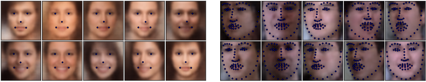
Figure 1: Samples $(\mathbf{d},\mathbf{h})\sim p(\mathbf{d},\mathbf{h})$ of two generative models trained on the CelebA dataset (top), and on the MultiPIE dataset (bottom). Note how the models consistently sample both the image and the corresponding pose.

The benefit of this hybrid approach is that it allows learning from partial observations in a principled manner and scales to realistic computer vision applications. In summary, our contributions are:

• Deriving a principled hybrid variational autoencoder model that allows for high-dimensional continuous output labels.

• Using unsupervised data as data-driven regularization for large scale deep learning models.

• Experimentally validating the improved generative model performance in terms of better likelihoods and improved sample quality for facial landmarks.

2 Full Variational Autoencoder Framework

We extend the deep VAE framework originally presented in Kingma and Welling (2014); Rezende et al. (2014); Doersch (2016) to the case of pairs of observations. This extension is technically straightforward and, like the VAE approach, has three components: first, a probabilistic model formulated as an infinite latent mixture model; second, an efficient approximate maximum likelihood learning procedure; and third, an effective variance reduction method that allows effective maximum likelihood training using backpropagation.

For the probabilistic model, we are interested in representing a distribution $p(\mathbf{d},\mathbf{h})$. Here $\mathbf{d}$ is an image, and $\mathbf{h}$ is an encoding of a continuous image label, e.g. a set of locations of the markers for face alignments. We define an infinite mixture model using an additional latent variable ${\mathbf{z}}$ as

$$p(\mathbf{d},\mathbf{h})=\int p_{\theta}(\mathbf{d},\mathbf{h}|{\mathbf{z}})\,p({\mathbf{z}})\,\textrm{d}{\mathbf{z}}.$$ (1)

The conditional distribution $p_{\theta}(\mathbf{d},\mathbf{h}|{\mathbf{z}})$ is described by a neural network and has parameters $\theta$ to be learned from a training data set. In practice this is implemented by outputting the parameters of a multivariate Normal distribution, $\mathcal{N}(\mu_{\theta}({\mathbf{z}}),\Sigma_{\theta}({\mathbf{z}}))$ so that the conditional likelihood $p_{\theta}(\mathbf{d},\mathbf{h}|{\mathbf{z}})$ can be computed easily. The distribution $p({\mathbf{z}})$ is fixed to be a multivariate standard Normal distribution, $p({\mathbf{z}})=\mathcal{N}(\mathbf{0},\mathbf{I})$. The above model is expressive, because it corresponds to an infinite Gaussian mixture model and hence can approximate complicated distributions.

To learn the parameters of the model using maximum likelihood, Kingma and Welling (2014); Rezende et al. (2014) introduce a tractable lower-bound on the log-likelihood. Consider the log-likelihood of a single joint training sample $(\mathbf{d},\mathbf{h})$. Using variational Bayesian bounding techniques (see Doersch (2016)) we can lower bound the log-likelihood via an auxiliary model $q({\mathbf{z}}|\mathbf{d},\mathbf{h})$ by

$$\log p(\mathbf{d},\mathbf{h})\geq \mathbb{E}_{{\mathbf{z}}\sim q_{\omega}({\mathbf{z}}|\mathbf{d},\mathbf{h})}\left[\log p_{\theta}(\mathbf{d},\mathbf{h}|{\mathbf{z}})\right]-D_{\textrm{KL}}(q_{\omega}({\mathbf{z}}|\mathbf{d},\mathbf{h})\|p({\mathbf{z}}))=:\mathcal{L}_{F}(\theta,\mathbf{d},\mathbf{h}),$$ (2)

where $D_{\textrm{KL}}$ is the Kullback-Leibler divergence between the variational distribution and the prior, which for the case of two Normal distributions has a simple analytic form.

\begin{overpic}[width=433.62pt]{figures/nn-figure.pdf} \end{overpic}

Figure 2: The architecture of the F-VAE deep generative neural network model we use to implement Equation (2). Here FC denotes a fully-connected neural network.

To optimize the bound (2) we can use stochastic gradient descent, approximating the expectation using a few samples, perhaps using only a single sample. A naive sampling approach would incur a high variance in the estimated gradients; the reparametrization trick (see Kingma and Welling (2014); Rezende et al. (2014)) allows significant variance reduction in estimating (2). In the following, we refer to the models trained using eq. 2 as Full VAE or F-VAE, as they use only fully observed data for training. Fig. 2 shows the architecture of the F-VAE model.

3 Hybrid Learning: Using Unlabeled Data

Obtaining a large amount of $\{\mathbf{d}_{i}\}$ is possible for many computer vision tasks; however, it may be expensive to collect large amounts of paired data $(\mathbf{d}_{i},\mathbf{h}_{i})$ because it involves some procedure for ground truth collection or manual labelling of images. In the case of abundant unlabeled data where only the image part is observed, we would like to train our model from both the expensive labeled set and the partially observed data.

Given an unlabeled image $\mathbf{d}$, we consider the marginal likelihood $p(\mathbf{d})$ of the image as

$$\log p(\mathbf{d})=\log\int\int p_{\theta}(\mathbf{d},\mathbf{h}|{\mathbf{z}})p({\mathbf{z}})\,\textrm{d}{\mathbf{z}}\,\textrm{d}\mathbf{h}.$$ (3)

The above is a difficult high-dimensional integration problem. In what follows, we drop neural network parameters $\theta$ and $w$ for brevity of notation. Using a variational Bayes bounding technique we derive a tractable lower bound on this marginal log-likelihood by introducing one auxiliary model, $q(\mathbf{h}|\mathbf{d})$ and reusing $q({\mathbf{z}}|\mathbf{d},\mathbf{h})$ introduced in the Full VAE framework, (2),

$$\log\int\int q(\mathbf{h}|\mathbf{d})\frac{p(\mathbf{d},\mathbf{h}|{\mathbf{z}})}{q(\mathbf{h}|\mathbf{d})}q({\mathbf{z}}|\mathbf{d},\mathbf{h})\frac{p({\mathbf{z}})}{q({\mathbf{z}}|\mathbf{d},\mathbf{h})}\,\textrm{d}{\mathbf{z}}\,\textrm{d}\mathbf{h}.$$ (4)

Replacing the integrals with expectations and moving the logarithm inside gives the variational lower bound on the log-likelihood:

$$\log p(\mathbf{d})\!\!\! = \!\!\!\log\mathbb{E}_{\mathbf{h}}\left[\mathbb{E}_{{\mathbf{z}}}\Big{[}\frac{p(\mathbf{d},\mathbf{h}|{\mathbf{z}})}{q(\mathbf{h}|\mathbf{d})}\frac{p({\mathbf{z}})}{q({\mathbf{z}}|\mathbf{d},\mathbf{h})}\Big{]}\right]\geq\mathbb{E}_{\mathbf{h}}\mathbb{E}_{{\mathbf{z}}}\left[\log\frac{p(\mathbf{d},\mathbf{h}|{\mathbf{z}})}{q(\mathbf{h}|\mathbf{d})}+\log\frac{p({\mathbf{z}})}{q({\mathbf{z}}|\mathbf{d},\mathbf{h})}\right]$$ (5)

$$= \!\!\!\mathbb{E}_{\mathbf{h}}\Big{[}\mathbb{E}_{{\mathbf{z}}}\Big{[}\log p(\mathbf{d},\mathbf{h}|{\mathbf{z}})-\log q(\mathbf{h}|\mathbf{d})\Big{]}-D_{\textrm{KL}}(q({\mathbf{z}}|\mathbf{d},\mathbf{h})\|p({\mathbf{z}}))\Big{]}.$$

Here, $\mathbb{E}_{\mathbf{h}}$ is shorthand for $\mathbb{E}_{\mathbf{h}\sim q(\mathbf{h}|\mathbf{d})}$, and likewise $\mathbb{E}_{{\mathbf{z}}}$ stands for $\mathbb{E}_{{\mathbf{z}}\sim q({\mathbf{z}}|\mathbf{d},\mathbf{h})}$. We rewrite (5) by recognizing the entropy term $H(q(\mathbf{h}|\mathbf{d}))=-\mathbb{E}_{{\mathbf{z}}}[\log q(\mathbf{d}|\mathbf{h})]$, giving

$$\log p(\mathbf{d})\geq\mathbb{E}_{\mathbf{h}}\Big{[}\mathbb{E}_{{\mathbf{z}}}\left[\log p_{\theta}(\mathbf{d},\mathbf{h}|{\mathbf{z}})\right]-D_{\textrm{KL}}(q({\mathbf{z}}|\mathbf{d},\mathbf{h})\|p({\mathbf{z}}))\Big{]}+H(q(\mathbf{h}|\mathbf{d}))\,=:\mathcal{L}_{P}(\theta,\mathbf{d}).$$ (6)

In our case, the entropy $H(q(\mathbf{h}|\mathbf{d}))$ is available as a simple analytic form because we use a multivariate Normal distribution for $q(\mathbf{h}|\mathbf{d})$. Note that $q(\mathbf{h}|\mathbf{d})$ represents essentially a discriminative model, implemented using a deep neural network.

We now combine $\mathcal{L}_{F}$ and $\mathcal{L}_{P}$ into one learning objective. For this, we assume we have a dataset $\{(\mathbf{d}_{i},\mathbf{h}_{i})\}_{i=1,\dots,n}$ of fully-observed samples and another dataset $\{(\mathbf{d}_{j})\}_{j=1,\dots,m}$ of partially-observed data, so that only $\mathbf{d}$ is observed. Typically $m\gg n$ because it is easier to obtain unlabeled images. Because both $\mathcal{L}_{F}$ and $\mathcal{L}_{P}$ are log-likelihood bounds for a single instance, one principled way to combine the two learning objectives is to simply sum them over all instances,

$$\mathcal{L}_{1}(\theta):=\sum_{i=1}^{n}\mathcal{L}_{F}(\theta,\mathbf{d}_{i},\mathbf{h}_{i})+\sum_{j=1}^{m}\mathcal{L}_{P}(\theta,\mathbf{d}_{j}).$$ (7)

While (7) is a valid log-likelihood bound, we found that empirically learning is faster when the relative contribution of each sum is weighted equally. We achieve this through the learning objective

$$\mathcal{L}(\theta):=\frac{1}{n}\sum_{i=1}^{n}\mathcal{L}_{F}(\theta,\mathbf{d}_{i},\mathbf{h}_{i})+\frac{1}{m}\sum_{j=1}^{m}\mathcal{L}_{P}(\theta,\mathbf{d}_{j}).$$ (8)

We optimize (8) using minibatch stochastic gradient descent, sampling one separate minibatch for each sum per iteration. We consider $\mathcal{L}(\theta)$ in (8) to be a hybrid learning objective, as it couples together generative and discriminative models. Hence the name of the model: Hybrid VAE (H-VAE).

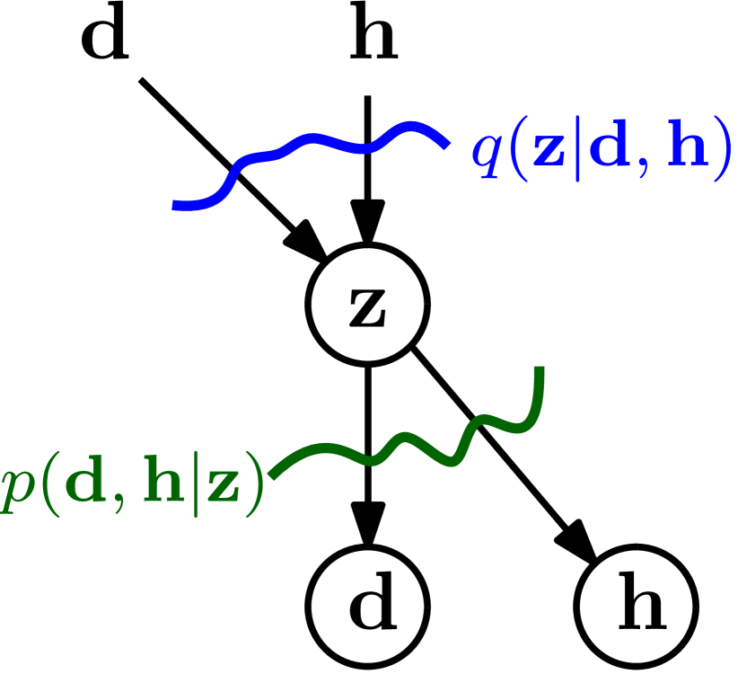
(a) Full VAE

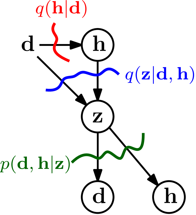
(b) Hybrid VAE

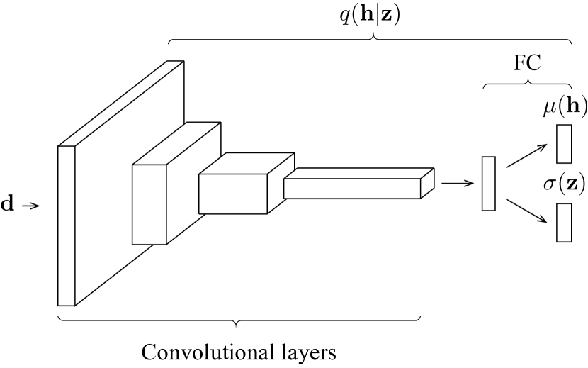
(c) Architecture of $\color[rgb]{1,0,0}q(\mathbf{h}|\mathbf{d})$

Figure 3: Extending the variational autoencoder (VAE) model to the case of hybrid labeled/unlabeled observations. (3(a)) the standard VAE model extended to the paired observation case: an encoder $q({\mathbf{z}}|\mathbf{d},\mathbf{h})$ and decoder $p(\mathbf{d},\mathbf{h}|{\mathbf{z}})$ mapping to/from a latent code ${\mathbf{z}}$; (3(b)) the hybrid VAE model introducing a discriminative variational model $q(\mathbf{h}|\mathbf{d})$ (3(c)) The architecture of the discriminative network.

We show in the experimental section that hybrid learning using (8) greatly improves the log-likelihood on the hold-out set of the generative model. Additionally we show that the use of a large set of partially observed instances prevents overfitting of the generative models. Fig. 3(a) and Fig. 3(b) outline the components of the F-VAE and H-VAE frameworks respectively.

3.1 Modeling Depth Images

Compared to natural images, depth images have the additional property that depth values could be unobserved. This is either because a pixel is outside the operating range of the camera or because the pixel is invalidated by the depth engine.

To model this effect accurately, we proceed in two steps: for each pixel, we first compute a probability of being observed, $p(\mathbf{b}|{\mathbf{z}})$, where $\mathbf{b}$ is a probability map with one probability $b_{u}\in[0,1]$ for each position $u$. If $b_{u}=1$ then the normal continuous model $p(d_{u}|{\mathbf{z}})$ is used, but if $b_{u}=0$, then the depth value is set to $d_{u}=\emptyset$, a symbolic “unobserved” value. Formally this corresponds to enlarging the domain of depth observations to $\mathbb{R}\cup\{\emptyset\}$ and using the probability model $p(\mathbf{d}|{\mathbf{z}})=\int p(\mathbf{d}|\mathbf{b},{\mathbf{z}})\,p(\mathbf{b}|{\mathbf{z}})\,\textrm{d}\mathbf{b}$. We can implement this simple model efficiently as a summation over two maps because there are only two states for each pixel.

4 Experiments

4.1 Implementation Details

An H-VAE model has three neural networks as shown in Fig. 3(b). Each of these networks uses either convolutional or deconvolutional subnetworks, and these parts closely follow the encoder-decoder architecture proposed in Radford et al. (2015). We visualize the network architectures in Fig. 2 and Fig. 3(c). Every convolutional layer doubles the number of channels, while shrinking the width and height by a factor of two. Deconvolutatal layers perform the opposite operation: they reduce the number of channels by the factor of two, but double the width and height by a factor of two.

Given a pair of $(\mathbf{d},\mathbf{h})$ the encoding network $q({\mathbf{z}}|\mathbf{d},\mathbf{h})$ independently processes $\mathbf{d}$ using the convolutional subnetwork, while $\mathbf{h}$ is processed by the three-layer fully-connected neural network (FC-NN). These two outputs are then concatenated and passed through another FC-NN, producing a diagonal multivariate Normal distribution over ${\mathbf{z}}$. The decoder network $p(\mathbf{d},\mathbf{h}|{\mathbf{z}})$ first processes ${\mathbf{z}}$ using an FC-NN, the pipeline then split, and the deconvolutional subnetwork is used to produce a diagonal multivariate Normal distribution over $\mathbf{d}$. The distribution over $\mathbf{h}$ is computed by yet another FC-NN, again as a diagonal multivariate Normal. We use ReLU activations (Nair and Hinton (2010)) throughout all the networks and every FC-NN hidden layer has 256 units. In every stochastic layer, we use unbiased estimates for the expectations by averaging three samples from the corresponding distribution. We implement the pipeline in Chainer (Tokui et al. (2015)) and train it end-to-end using SGD with learning rate $0.01$ and momentum $0.9$.

4.2 Datasets

Previous work on generative models used data sets such as MNIST (LeCun et al. (1998)) and SVHN (Netzer et al. (2011)) for evaluating their models. In our work, however, these datasets do not allow us to show the benefits of the proposed H-VAE approach, as they include categorical labels only, whereas our method extends the standard VAE framework to deal with continuous annotation $\mathbf{h}$.

We evaluate our method on two up-to-date datasets used in the computer vision community. To simulate partially observed samples, we shuffle the dataset and split it into fully- and partially-observed subsets and separate a holdout test set, not available during training.

MultiPIE. The MultiPIE (Gross et al. (2010)) dataset consists of face images of 337 subjects taken under different pose, illumination and expressions. The pose range contains 15 discrete views, capturing a face profile-to-profile. Illumination changes were modeled using 19 flashlights located in different places of the room. The database has been extensively used in the community for face alignment (Xiong and De la Torre (2013); Zhu and Ramanan (2012); Tulyakov et al. (2017a)). For our purposes we use only the views annotated either with 68 or 66-points markup, in total producing 47250 images. We drop the inner mouth corner points, so that all the images have the same 66-point markup. Images were cropped around the landmarks and downscaled to 48$\times$48 size. We reserve 2K $(\mathbf{d},\mathbf{h})$ pairs from the MultiPIE dataset for testing purposes.

CelebA face dataset. The CelebA (Liu et al. (2015)) is a large scale face attributes dataset containing more that 200K celebrity images annotated with 40 attributes (such as eyeglasses, pointy nose etc.) and 5 landmark locations (eyes, nose, mouth corners). It contains more than 10K distinct identities. As in Lamb et al. (2016) we center and crop all images around the face and resize to $64\times 64$. We use the provided landmarks as continuous labels $\mathbf{h}$. The testing set consists of 10K fully observed instances.

NYU Hand Pose dataset. The NYU Hand Pose Dataset (Tompson et al. (2014)) contains 72757 training frames of RGBD data and 8252 testing set frames. For every frame, the RGBD data from 3 kinects is available. In our experiments we use only depth frames captured from the front view. We resize depth maps to $128\times 128$ and preprocess the depth values using the code from Oberweger et al. (2015).

4.3 Quantitative Evaluation

Table 1: Comparison of F-VAE and H-VAE models on three datasets: (1(a)) MultiPIE, (1(b)) CelebA, (1(c)) NYU Hand Pose. The number of fully observed samples used for training is denoted by $n$, while $m$ corresponds to the total number of partially observed instances. We report the task-loss $E_{\text{task}}$ and the negative log-likelihood of the fully observed testing data computed using eq. 2.

(a) MultiPIE

	$n$	$m$	$E_{\text{task}}$	$-\log p(\mathbf{d},\mathbf{h})$
F-VAE	5k	-	-	-23.00
	15k	-	-	-27.33
	30k	-	-	-31.25
H-VAE	500	5k	0.1162	-20.43
	500	30k	0.1457	-25.75
	5k	5k	0.0935	-28.29
	5k	30k	0.0845	-32.36

(b) CelebA

	$n$	$m$	$E_{\text{task}}$	$-\log p(\mathbf{d},\mathbf{h})$
F-VAE	15k	-	-	-3.49
	30k	-	-	-7.40
	50k	-	-	-7.19
	100k	-	-	-8.15
H-VAE	5k	100k	0.1425	-6.90
	5k	150k	0.1420	-6.98
	15k	15k	0.1181	-5.90
	15k	100k	0.0929	-9.08

(c) NYU Hand Pose

	$n$	$m$	$E_{\text{task}}$	$-\log p(\mathbf{d},\mathbf{h})$
F-VAE	10k	-	-	29.31
	30k	-	-	26.27
H-VAE	10k	10k	4.54	29.31
	10k	20k	4.82	25.89
	10k	30k	4.56	21.13
	30k	10k	4.82	19.20
	30k	20k	4.56	18.42
	30k	30k	4.56	14.11

A commonly accepted comparison procedure for generative modeling is evaluation of the negative log-likelihood (NLL) on the testing data (Gneiting and Raftery (2007); Lamb et al. (2016); Kingma et al. (2016)). We compute the NLL using Eq. (2) on the same fully observed testing data for each model. This metric, however, is difficult to interpret, requiring visual samples from the model to assess their quality. Therefore, we additionally report the task-loss $E_{\text{task}}$. The task-loss in the case of face alignment is the average point-to-point Euclidean distance, normalized by the interocular distance (Tulyakov and Sebe (2015); Trigeorgis et al. (2016)). For hand pose experiment we report the average $L_{2}$ distance between the ground truth and the prediction. We report the task-loss by evaluating the mean of $q(\mathbf{h}|\mathbf{d})$ trained using the hybrid objective (8). This metric is not available for the F-VAE models. For brevity reasons, we denote F-VAE($n$) as a F-VAE model trained using $n$ fully observed samples, and similarly H-VAE($n$, $m$) trained with $n$ fully- and $m$ partially-observed instances.

Table 1(a) compares multiple F-VAE models against the proposed H-VAE models on the MultiPIE dataset. Clearly, using a hybrid learning objective with partially observed data helps drastically improve the likelihood: the H-VAE(500, 30K) model outperforms the F-VAE(5K). Similarly, the H-VAE(5K, 30K) model shows better NLL as compared to F-VAE(30K).

The same holds for the CelebA dataset, as seen in table 1(b). The F-VAE(5K) model is not able to accurately learn the distribution. Instead, it overfits, leading to the worse NLL. In contrast, the H-VAE(5K, 15K) has comparable results with the F-VAE(15K), advocating for the use of inexpensive partial observations. Additionally, H-VAE(30K, 150K) outperforms F-VAE(150K). Similar results can be observed on the NYU Hand Pose dataset (Table 1(c)), where the H-VAE(10k, 10k) models shows NLL comparable to F-VAE(30K), and clearly the model having the most of fully observed and partially observed data scores best.

4.4 Qualitative Evaluation

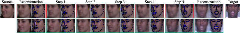
(a) Samples the first row (red) for every example are obtained using the F-VAE(5K) model, the bottom row (green) is produced by the H-VAE(5K, 30K) model. Both models were trained on the MultiPIE dataset.

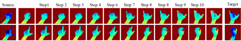
(b) Interpolating depth images using the H-VAE(30K, 30K) model trained on the NYU Hand Pose dataset.

Figure 4: Selected examples showing interpolations. For every interpolation, the source and the target images are taken from the testing set, projected to and reconstructed from the latent space, interpolation is performed from the source to the target.

One of the key benefits of generative modeling is the ability to analyze the learned distribution by performing sampling. Since ${\mathbf{z}}\sim\mathcal{N}(\mathbf{0},\mathbf{I})$ one can sample ${\mathbf{z}}$ and then sample $(\mathbf{d},\mathbf{h})\sim p(\mathbf{d},\mathbf{h}|{\mathbf{z}})$ to get an image and its label. Fig. 1 shows several examples of that. Note how a generative model can consistently represent pose and image information. The CelebA dataset consists of public images of celebrities, and therefore is biased towards smiling faces. The bottom half of Fig. 1 shows samples from the distribution learned using the MultiPIE dataset. Since the MultiPIE dataset consists of multiple poses, illuminations and expressions, the model is able to encode them. Interestingly, one can project two images onto the ${\mathbf{z}}$-space by sampling ${\mathbf{z}}\sim q({\mathbf{z}}|\mathbf{d},\mathbf{h})$ and analyze the structure of the learned space by linearly interpolating between the two points.

Source-target interpolation on the MultiPIE dataset is given in Fig. 4(a). The models were trained on the MultiPIE dataset. For this example, the top row is obtained using the F-VAE(5K) model that saw only 5K labeled examples during training. The bottom row is produced using the model trained on 5K fully observed samples and 30K of partial observations (H-VAE(5K, 30K)). Clearly, partial observations significantly improve image quality, making the texture less blurry, and better representing facial expressions. Interestingly, both models gradually transform between images (i.e. open a mouth or rotate a face), indicating that by exploring the latent representation one can generate plausible face trajectories. It also shows that, in general, useful semantics are linearized in the hidden representation of the model.

Similar interpolation on the NYU Hand Pose dataset is given in Fig. 4(b). Interestingly, gesture transformation is encoded in the representation. Traversing a line transforms to bending or unbending fingers in the image space.

5 Related work

We first discuss existing state-of-the-art deep generative models. Since our formulation is joint in terms of images and their labels we review previous attempts to create such a joint representation. Additionally, as our model is a hybrid consisting of discriminative and generative parts we outline previous related works in this area.

5.1 Deep Generative Models

Current research focuses on two classes of models, generative adversarial networks and variational autoencoders.

Generative adversarial networks (GAN) were proposed recently in the machine learning community as neural architectures for generative models (Goodfellow et al. (2014)). In a GAN two networks are trained together, competing against each other: the generator tries to produce realistic samples, e.g. images; the adversary tries to distinguish generated samples from training samples. Formally, this yields a challenging $\min-\max$ optimization problem and a variety of techniques have been proposed to stabilize learning in GANs, see Salimans et al. (2016); Sønderby et al. (2016); Metz et al. (2016).

Despite this difficulty, multiple extensions of the original work appeared in the literature. Deep convolutional generative adversarial network in Radford et al. (2015) and Denton et al. (2015) show surprisingly photo-realistic and sharp image samples as compared to previous works. The authors provide multiple architectural guidelines that improve the overall quality of the sampled images. As a result the models are able to produce samples for trajectories in the latent space, showing the internal structure of the learned space. The work in Nowozin et al. (2016) shows that GANs can be viewed as a special case of a more general variational divergence estimation approach. Further examples of GANs include generating images of birds from textual description, Reed et al. (2016), styling images, Ulyanov et al. (2016), and video generation, Vondrick et al. (2016); Tulyakov et al. (2017b).

Variational autoencoders were introduced independently by two groups (Kingma and Welling (2014); Rezende et al. (2014)). VAEs maximize a variational lower bound on the log-likelihood of the data. Similarly to GANs, this is a recently emerged and rapidly evolving area of generative modeling.

Since the original works, there have been many extensions introduced. The work in Kingma et al. (2014) extends the VAE framework to semi-supervised learning. In Maaløe et al. (2015) the idea of semi-supervised learning is exploited further, by introducing and auxiliary variables improving the variational approximation. The Deep Recurrent Attentive Writer (DRAW), Gregor et al. (2015), employs recurrent neural networks acting as encoder and decoder, in a way mimicking the foveation of the human eye. Inverse Autoregressive Flow (IAF) presented in Kingma et al. (2016) and auxiliary variables (Maaløe et al. (2015)) are two approaches to further improve the quality of the variational approximation and quality of the images generated by the model. Another recent attempt at improving inferences is to consider hybrid GAN-VAE models as in Wu et al. (2016).

5.2 Hybrid Models

Learning a probabilistic model from different levels of annotations has been proposed earlier in Navaratnam et al. (2007); in particular, using Gaussian processes (GP) the authors report improved person tracking performance. However, while GPs are analytically tractable they do not scale well and the work is limited to use very small data sets.

In Lasserre et al. (2006) the authors consider the problem of combining a generative models $p(\mathbf{d},\mathbf{h})$ with a discriminative model $p_{d}(\mathbf{h}|\mathbf{d})$. They achieve this in a satisfying manner by creating a new model whose likelihood function can smoothly balance between training objectives of the generative and discriminative models. However, the proposed coupling prior of Lasserre et al. (2006) is not useful in the context of neural networks because Euclidean distance in the parameter vector of two neural networks does not measure useful differences in the function realized by the neural network. The model is shown to work well for discrete labels $\mathbf{h}$ in the empirical study (Druck et al. (2007)).

Whereas the above work addresses semi-supervised learning with the goal to improve the predictive performance of $p(\mathbf{h}|\mathbf{d})$, our main interest is in improving the performance of the generative model $p(\mathbf{d},\mathbf{h})$. Moreover, our work shows to to handle the marginal likelihood over $\mathbf{h}$ in an efficient ant tractable manner.

6 Conclusions

We demonstrated a scalable and practical way to learn rich generative models of multiple output modalities. Compared to the ordinary deep generative model our hybrid VAE model does not require fully labelled observations for all samples. Because the hybrid VAE model derives from the principled variational autoencoder model it can represent complex distributions of images and pose and could be easily adapted to other modalities.

Our experiments demonstrate that when mixing fully labelled with unlabelled data the hybrid learning greatly improves over the standard generative model which can use only the fully labelled data. The improvement is both in terms of test set log-likelihood and in the quality of image samples generated by the model.

We believe that hybrid generative models such as our hybrid VAE model address one of the key limitation of deep learning: the requirement of having large scale labelled data sets. We hope that hybrid VAE model will enable large scale learning from unsupervised data for a variety of computer vision tasks.

References

- Denton et al. [2015] Emily L Denton, Soumith Chintala, Rob Fergus, et al. Deep generative image models using a laplacian pyramid of adversarial networks. In NIPS, 2015.
- Doersch [2016] Carl Doersch. Tutorial on Variational Autoencoders. arXiv, pages 1–23, 2016. URL http://arxiv.org/abs/1606.05908.
- Druck et al. [2007] Gregory Druck, Chris Pal, Andrew McCallum, and Xiaojin Zhu. Semi-supervised classification with hybrid generative/discriminative methods. In Proceedings of the 13th ACM SIGKDD international conference on Knowledge discovery and data mining, pages 280–289. ACM, 2007.
- Gneiting and Raftery [2007] Tilmann Gneiting and Adrian E Raftery. Strictly proper scoring rules, prediction, and estimation. Journal of the American Statistical Association, 102(477):359–378, 2007.
- Goodfellow et al. [2014] Ian Goodfellow, Jean Pouget-Abadie, Mehdi Mirza, Bing Xu, David Warde-Farley, Sherjil Ozair, Aaron Courville, and Yoshua Bengio. Generative adversarial nets. In NIPS, pages 2672–2680. 2014.
- Gregor et al. [2015] Karol Gregor, Ivo Danihelka, Alex Graves, Danilo Jimenez Rezende, and Daan Wierstra. Draw: A recurrent neural network for image generation. arXiv preprint arXiv:1502.04623, 2015.
- Gross et al. [2010] Ralph Gross, Iain Matthews, Jeffrey Cohn, Takeo Kanade, and Simon Baker. Multi-pie. Image and Vision Computing, 28(5):807–813, 2010.
- Kingma and Welling [2014] Diederik P Kingma and Max Welling. Auto-Encoding Variational Bayes. In ICLR, 2014.
- Kingma et al. [2014] Diederik P Kingma, Danilo J Rezende, Shakir Mohamed, and Max Welling. Semi-Supervised Learning with Deep Generative Models. In NIPS, 2014.
- Kingma et al. [2016] Diederik P Kingma, Tim Salimans, and Max Welling. Improving Variational Inference with Inverse Autoregressive Flow. In NIPS, 2016.
- Lamb et al. [2016] Alex Lamb, Vincent Dumoulin, and Aaron Courville. Discriminative regularization for generative models. arXiv preprint arXiv:1602.03220, 2016.
- Lasserre et al. [2006] Julia A. Lasserre, Christopher M. Bishop, and Thomas P. Minka. Principled hybrids of generative and discriminative models. In CVPR, 2006.
- LeCun et al. [1998] Yann LeCun, Corinna Cortes, and Christopher JC Burges. The mnist database of handwritten digits, 1998.
- Liu et al. [2015] Ziwei Liu, Ping Luo, Xiaogang Wang, and Xiaoou Tang. Deep learning face attributes in the wild. In ICCV, pages 3730–3738, 2015.
- Maaløe et al. [2015] Lars Maaløe, Casper Kaae Sønderby, Søren Kaae Sønderby, and Ole Winther. Auxiliary Deep Generative Models. In NIPS workshop, 2015.
- Metz et al. [2016] Luke Metz, Ben Poole, David Pfau, and Jascha Sohl-Dickstein. Unrolled generative adversarial networks. arXiv preprint arXiv:1611.02163, 2016.
- Nair and Hinton [2010] Vinod Nair and Geoffrey E Hinton. Rectified linear units improve restricted boltzmann machines. In ICML, 2010.
- Navaratnam et al. [2007] Ramanan Navaratnam, Andrew W Fitzgibbon, and Roberto Cipolla. The joint manifold model for semi-supervised multi-valued regression. In CVPR. IEEE, 2007.
- Netzer et al. [2011] Yuval Netzer, Tao Wang, Adam Coates, Alessandro Bissacco, Bo Wu, and Andrew Y Ng. Reading digits in natural images with unsupervised feature learning. 2011.
- Nowozin et al. [2016] Sebastian Nowozin, Botond Cseke, and Ryota Tomioka. f-GAN: Training generative neural samplers using variational divergence minimization. In NIPS, 2016.
- Oberweger et al. [2015] Markus Oberweger, Paul Wohlhart, and Vincent Lepetit. Hands deep in deep learning for hand pose estimation. arXiv preprint arXiv:1502.06807, 2015.
- Radford et al. [2015] Alec Radford, Luke Metz, and Soumith Chintala. Unsupervised representation learning with deep convolutional generative adversarial networks. arXiv preprint arXiv:1511.06434, 2015.
- Reed et al. [2016] Scott Reed, Zeynep Akata, Xinchen Yan, Lajanugen Logeswaran, Bernt Schiele, and Honglak Lee. Generative adversarial text to image synthesis. arXiv preprint arXiv:1605.05396, 2016.
- Rezende et al. [2014] D J Rezende, S Mohamed, and D Wierstra. Stochastic backpropagation and approximate inference in deep generative models. 2014.
- Salimans et al. [2016] Tim Salimans, Ian Goodfellow, Wojciech Zaremba, Vicki Cheung, Alec Radford, and Xi Chen. Improved techniques for training gans. In NIPS, 2016.
- Sønderby et al. [2016] Casper Kaae Sønderby, Jose Caballero, Lucas Theis, Wenzhe Shi, and Ferenc Huszár. Amortised map inference for image super-resolution. arXiv preprint arXiv:1610.04490, 2016.
- Tokui et al. [2015] Seiya Tokui, Kenta Oono, Shohei Hido, and Justin Clayton. Chainer: a next-generation open source framework for deep learning. In NIPS, 2015.
- Tompson et al. [2014] Jonathan Tompson, Murphy Stein, Yann Lecun, and Ken Perlin. Real-time continuous pose recovery of human hands using convolutional networks. ACM Transactions on Graphics, 33, August 2014.
- Trigeorgis et al. [2016] George Trigeorgis, Patrick Snape, Mihalis A Nicolaou, Epameinondas Antonakos, and Stefanos Zafeiriou. Mnemonic descent method: A recurrent process applied for end-to-end face alignment. In CVPR, 2016.
- Tulyakov and Sebe [2015] Sergey Tulyakov and Nicu Sebe. Regressing a 3d face shape from a single image. In ICCV, pages 3748–3755. IEEE, 2015.
- Tulyakov et al. [2017a] Sergey Tulyakov, László Jeni, Jeffrey Cohn, and Nicu Sebe. Viewpoint-consistent 3d face alignment. IEEE Transactions on Pattern Analysis and Machine Intelligence, 09 2017a.
- Tulyakov et al. [2017b] Sergey Tulyakov, Ming-Yu Liu, Xiaodong Yang, and Jan Kautz. Mocogan: Decomposing motion and content for video generation. arXiv preprint arXiv:1707.04993, 2017b.
- Ulyanov et al. [2016] Dmitry Ulyanov, Vadim Lebedev, Andrea Vedaldi, and Victor Lempitsky. Texture networks: Feed-forward synthesis of textures and stylized images. arXiv preprint arXiv:1603.03417, 2016.
- Vondrick et al. [2016] Carl Vondrick, Hamed Pirsiavash, and Antonio Torralba. Generating videos with scene dynamics. arXiv preprint arXiv:1609.02612, 2016.
- Wu et al. [2016] Jiajun Wu, Chengkai Zhang, Tianfan Xue, William T Freeman, and Joshua B Tenenbaum. Learning a probabilistic latent space of object shapes via 3d generative-adversarial modeling. arXiv preprint arXiv:1610.07584, 2016.
- Xiong and De la Torre [2013] Xuehan Xiong and Fernando De la Torre. Supervised descent method and its applications to face alignment. In CVPR, pages 532–539, 2013.
- Zhu and Ramanan [2012] Xiangxin Zhu and Deva Ramanan. Face detection, pose estimation, and landmark localization in the wild. In CVPR, pages 2879–2886, 2012.