All-Helicity Symbol Alphabets from Unwound Amplituhedra

Abstract

We review an algorithm for determining the branch points of general amplitudes in planar $\mathcal{N}=4$ super-Yang–Mills theory from amplituhedra. We demonstrate how to use the recent reformulation of amplituhedra in terms of ‘sign flips’ in order to streamline the application of this algorithm to amplitudes of any helicity. In this way we recover the known branch points of all one-loop amplitudes, and we find an ‘emergent positivity’ on boundaries of amplituhedra.

1 Introduction

Physical principles impose strong constraints on the scattering amplitudes of elementary particles. For example, when working at finite order in perturbation theory, unitarity and locality appear to constrain amplitudes to be holomorphic functions with poles and branch points at precisely specified locations in the space of complexified kinematic data describing the configuration of particles. Indeed, it has been a long-standing goal to understand how to use the tightly prescribed analytic structure of scattering amplitudes to determine them directly, without relying on traditional (and, often computationally complex) Feynman diagram techniques.

The connection between the physical and mathematical structure of scattering amplitudes has been especially well studied in planar $\mathcal{N}=4$ super-Yang–Mills Brink:1976bc SYM theory in four spacetime dimensions, where the analytic structure of amplitudes is especially tame. The overall aim of this paper, its predecessors Dennen:2015bet ; Dennen:2016mdk , and its descendant(s), is to ask a question that might be hopeless in another, less beautiful quantum field theory: can we understand the branch cut structure of general scattering amplitudes in SYM theory?

The motivation for asking this question is two-fold. The first is the expectation that the rich mathematical structure that underlies the integrands of SYM theory (the rational $4L$-forms that arise from summing $L$-loop Feynman diagrams, prior to integrating over loop momenta) is reflected in the corresponding scattering amplitudes. For example, it has been observed that both integrands ArkaniHamed:2012nw and amplitudes Golden:2013xva ; Golden:2014pua ; Drummond:2017ssj are deeply connected to the mathematics of cluster algebras.

Second, on a more practical level, knowledge of the branch cut structure of amplitudes is the key ingredient in the amplitude bootstrap program, which represents the current state of the art for high loop order amplitude calculations in SYM theory. In particular the hexagon bootstrap (see for example Dixon:2014xca ), which has succeeded in computing all six-particle amplitudes through five loops Caron-Huot:2016owq , is predicated on the hypothesis that at any loop order, these amplitudes can have branch points only on 9 specific loci in the space of external data. Similarly the heptagon bootstrap Drummond:2014ffa , which has revealed the symbols of the seven-particle four-loop MHV and three-loop NMHV amplitudes Dixon:2016nkn , assumes 42 particular branch points. One result we hope follows from understanding the branch cut structure of general amplitudes in SYM theory is a proof of this counting to all loop order for six- and seven-particle amplitudes.

It is a general property of quantum field theory (see for example Cutkosky:1960sp ; ELOP ) that the locations of singularities of an amplitude can be determined from knowledge of the poles of its integrand by solving the Landau equations Landau:1959fi . Constructing explicit representations for integrands can be a challenging problem in general, but in SYM theory this can be side-stepped by using various on-shell methods Bern:1994cg ; Cachazo:2004kj ; Britto:2005fq ; Elvang:2013cua to efficiently determine the locations of integrand poles. This problem is beautifully geometrized by amplituhedra Arkani-Hamed:2013jha , which are spaces encoding representations of integrands in such a way that the boundaries of an amplituhedron correspond precisely to the poles of the corresponding integrand. Therefore, as pointed out in Dennen:2016mdk (which we now take as our conceptual framework), the Landau equations can be interpreted as defining a map that associates to any boundary of an amplituhedron the locus in the space of external data where the corresponding amplitude has a singularity.

Only MHV amplitudes were considered in Dennen:2016mdk . In this paper we show how to extend the analysis to amplitudes of arbitrary helicity. This is greatly aided by a recent combinatorial reformulation of amplituhedra in terms of “sign flips” Arkani-Hamed:2017vfh . As a specific application of our algorithm we classify the branch points of all one-loop amplitudes in SYM theory. Although the singularity structure of these amplitudes is of course well-understood (see for example tHooft:1978jhc ; Bern:1993kr ; Bern:1994zx ; Bern:1994ju ; Brandhuber:2004yw ; Bern:2004ky ; Britto:2004nc ; Bern:2004bt ; Ellis:2007qk ), this exercise serves a useful purpose in preparing a powerful toolbox for the sequel Prlina:2017tvx to this paper where we will see that boundaries of one-loop amplituhedra are the basic building blocks at all loop order. In particular we find a surprising ‘emergent positivity’ on boundaries of one-loop amplituhedra that allows boundaries to be efficiently mapped between different helicity sectors, and recycled to higher loop levels.

The rest of this paper is organized as follows. In Sec. 2 we review relevant definitions and background material and summarize the general procedure for finding singularities of amplitudes. In Secs. 3 and 4 we classify the relevant boundaries of all one-loop amplituhedra. Section 5 outlines a simple graphical notation for certain boundaries and shows that the one-loop boundaries all assemble into a simple graphical hierarchy which will prove useful for organizing higher-loop computations. In Sec. 6 we show how to formulate and efficiently solve the Landau equations directly in momentum twistor space, thereby completing the identification of all branch points of one-loop amplitudes. The connection between these results and symbol alphabets is discussed in Sec. 7.

2 Review

This section provides a thorough introduction to the problem our work aims to solve. The concepts and techniques reviewed here will be illuminated in subsequent sections via several concrete examples.

2.1 The Kinematic Domain

Scattering amplitudes are (in general multivalued) functions of the kinematic data (the energies and momenta) describing some number of particles participating in some scattering process. Specifically, amplitudes are functions only of the kinematic information about the particles entering and exiting the process, called external data in order to distinguish it from information about virtual particles which may be created and destroyed during the scattering process itself. A general scattering amplitude in SYM theory is labeled by three integers: the number of particles $n$, the helicity sector $0\leq\textrm{k}\leq n-4$, and the loop order $L\geq 0$, with $L=0$ called tree level and $L>0$ called $L$-loop level. Amplitudes with $\textrm{k}=0$ are called maximally helicity violating (MHV) while those with $\textrm{k}>0$ are called (next-to-)${}^{\textrm{k}}$maximally helicity violating ($\textrm{N}^{\textrm{k}}\textrm{MHV}$).

The kinematic configuration space of SYM theory admits a particularly simple characterization: $n$-particle scattering amplitudes are multivalued functions on $\operatorname{Conf}_{n}(\mathbb{P}^{3})$, the space of configurations of $n$ points in $\mathbb{P}^{3}$ Golden:2013xva . A generic point in $\operatorname{Conf}_{n}(\mathbb{P}^{3})$ may be represented by a collection of $n$ homogeneous coordinates $Z_{a}^{I}$ on $\mathbb{P}^{3}$ (here $I\in\{1,\ldots,4\}$ and $a\in\{1,\ldots,n\}$) called momentum twistors Hodges:2009hk , with two such collections considered equivalent if the corresponding $4\times n$ matrices $Z\equiv(Z_{1}\cdots Z_{n})$ differ by left-multiplication by an element of $\operatorname{GL}(4)$. We use the standard notation

$$\langle a\,b\,c\,d\rangle=\epsilon_{IJKL}Z_{a}^{I}Z_{b}^{J}Z_{c}^{K}Z_{d}^{L}$$ (1)

for the natural $\operatorname{SL}(4)$-invariant four-bracket on momentum twistors and use the shorthand $\langle\cdots\,\overline{a}\,\cdots\rangle=\langle\cdots a{-}1\,a\,a{+}1\cdots\rangle$, with the understanding that all particle labels are always taken mod $n$. We write $(a\,b)$ to denote the line in $\mathbb{P}^{3}$ containing $Z_{a}$ and $Z_{b}$, $(a\,b\,c)$ to denote the plane containing $Z_{a},Z_{b}$ and $Z_{c}$, and so $\overline{a}$ denotes the plane $(a{-}1\,a\,a{+}1)$. The bar notation is motivated by parity, which is a $\mathbb{Z}_{2}$ symmetry of SYM theory that maps $\textrm{N}^{\textrm{k}}\textrm{MHV}$ amplitudes to $\textrm{N}^{n-\textrm{k}-4}\textrm{MHV}$ amplitudes while mapping the momentum twistors according to $\{Z_{a}\}\mapsto\{W_{a}=*(a{-}1\,a\,a{+}1)\}$.

When discussing $\textrm{N}^{\textrm{k}}\textrm{MHV}$ amplitudes it is conventional to consider an enlarged kinematic space where the momentum twistors are promoted to homogeneous coordinates $\mathcal{Z}_{a}$, bosonized momentum twistors Arkani-Hamed:2013jha on $\mathbb{P}^{\textrm{k}+3}$ which assemble into an $n\times(\textrm{k}+4)$ matrix $\mathcal{Z}\equiv(\mathcal{Z}_{1}\cdots\mathcal{Z}_{n})$. The analog of Eq. (1) is then the $\operatorname{SL}(\textrm{k}+4)$-invariant bracket which we denote by $[\cdot]$ instead of $\langle\cdot\rangle$. Given some $\mathcal{Z}$ and an element of the Grassmannian $\operatorname{Gr}(\textrm{k},\textrm{k}+4)$ represented by a $\textrm{k}\times(\textrm{k}+4)$ matrix $Y$, one can obtain an element of $\operatorname{Conf}_{n}(\mathbb{P}^{3})$ by projecting onto the complement of $Y$. The four-brackets of the projected external data obtained in this way are given by

$$\langle a\,b\,c\,d\rangle\equiv[Y\,\mathcal{Z}_{a}\,\mathcal{Z}_{b}\,\mathcal{Z}_{c}\,\mathcal{Z}_{d}]\,.$$ (2)

Tree-level amplitudes are rational functions of the brackets while loop-level amplitudes have both poles and branch cuts, and are properly defined on an infinitely-sheeted cover of $\operatorname{Conf}_{n}(\mathbb{P}^{3})$. For each k there exists an open set $\mathcal{D}_{n,\textrm{k}}\subset\operatorname{Conf}_{n}(\mathbb{P}^{3})$ called the principal domain on which amplitudes are known to be holomorphic and non-singular. Amplitudes are initially defined only on $\mathcal{D}_{n,\textrm{k}}$ and then extended to all of (the appropriate cover of) $\operatorname{Conf}_{n}(\mathbb{P}^{3})$ by analytic continuation.

A simple characterization of the principal domain for $n$-particle $\textrm{N}^{\textrm{k}}\textrm{MHV}$ amplitudes was given in Arkani-Hamed:2017vfh : $\mathcal{D}_{n,\textrm{k}}$ may be defined as the set of points in $\operatorname{Conf}_{n}(\mathbb{P}^{3})$ that can be represented by a $Z$-matrix with the properties

1. $\langle a\,a{+}1\,b\,b{+}1\rangle>0$ for all $a$ and $b\not\in\{a{-}1,a,a{+}1\}$, and

2. the sequence $\langle 1\,2\,3\,\bullet\rangle$ has precisely k sign flips,

where we use the notation $\bullet\in\{1\,,2\,,\ldots\,,n\}$ so that

$$\langle 1\,2\,3\,\bullet\rangle\equiv\{0,0,0,\langle 1\,2\,3\,4\rangle,\langle 1\,2\,3\,5\rangle,\ldots,\langle 1\,2\,3\,n\rangle\}\,.$$ (3)

It was also shown that an alternate but equivalent condition is to say that the sequence $\langle a\,a{+}1\,b\,\bullet\rangle$ has precisely k sign flips for all $a,b$ (omitting trivial zeros, and taking appropriate account of the twisted cyclic symmetry where necessary). The authors of Arkani-Hamed:2017vfh showed, and we review in Sec. 2.2, that for $Y$’s inside an N${}^{\textrm{k}}$MHV amplituhedron, the projected external data have the two properties above.

2.2 Amplituhedra …

A matrix is said to be positive or non-negative if all of its ordered maximal minors are positive or non-negative, respectively. In particular, we say that the external data are positive if the $n\times(\textrm{k}+4)$ matrix $\mathcal{Z}$ described in the previous section is positive.

A point in the $n$-particle $\textrm{N}^{\textrm{k}}\textrm{MHV}$ $L$-loop amplituhedron $\mathcal{A}_{n,\textrm{k},L}$ is a collection $(Y,\mathcal{L}^{(\ell)})$ consisting of a point $Y\in\operatorname{Gr}(\textrm{k},\textrm{k}+4)$ and $L$ lines $\mathcal{L}^{(1)},\ldots,\mathcal{L}^{(L)}$ (called the loop momenta) in the four-dimensional complement of $Y$. We represent each $\mathcal{L}^{(\ell)}$ as a $2\times(\textrm{k}+4)$ matrix with the understanding that these are representatives of equivalence classes under the equivalence relation that identifies any linear combination of the rows of $Y$ with zero.

For given positive external data $\mathcal{Z}$, the amplituhedron $\mathcal{A}_{n,\textrm{k},L}(\mathcal{Z})$ was defined in Arkani-Hamed:2013jha for $n\geq 4$ as the set of $(Y,\mathcal{L}^{(\ell)})$ that can be represented as

$$Y =C\mathcal{Z}\,,$$ (4)

$$\mathcal{L}^{(\ell)} =D^{(\ell)}\mathcal{Z}\,,$$ (5)

in terms of a $\textrm{k}\times n$ real matrix $C$ and $L$ $2\times n$ real matrices $D^{(\ell)}$ satisfying the positivity property that for any $0\leq m\leq L$, all $(2m+\textrm{k})\times n$ matrices of the form

$$\left(\begin{matrix}D^{(i_{1})}\cr D^{(i_{2})}\cr\vdots\cr D^{(i_{m})}\cr C\end{matrix}\right)$$ (6)

are positive. The $D$-matrices are understood as representatives of equivalence classes and are defined only up to translations by linear combinations of rows of the $C$-matrix.

One of the main results of Arkani-Hamed:2017vfh was that amplituhedra can be characterized directly by (projected) four-brackets, Eq. (2), without any reference to $C$ or $D^{(\ell)}$’s, by saying that for given positive $\mathcal{Z}$, a collection $(Y,\mathcal{L}^{(\ell)})$ lies inside $\mathcal{A}_{n,\textrm{k},L}(\mathcal{Z})$ if and only if

1. the projected external data lie in the principal domain $\mathcal{D}_{n,\textrm{k}}$,

2. $\langle\mathcal{L}^{(\ell)}\,a\,a{+}1\rangle>0$ for all $\ell$ and $a$,

3. for each $\ell$, the sequence $\langle\mathcal{L}^{(\ell)}\,1\,\bullet\rangle$ has precisely $\textrm{k}+2$ sign flips, and

4. $\langle\mathcal{L}^{(\ell_{1})}\,\mathcal{L}^{(\ell_{2})}\rangle>0$ for all $\ell_{1}\neq\ell_{2}$.

Here the notation $\langle\mathcal{L}\,a\,b\rangle$ means $\langle A\,B\,a\,b\rangle$ if the line $\mathcal{L}$ is represented as $(A\,B)$ for two points $A,B$. It was also shown that items 2 and 3 above are equivalent to saying that the sequence $\langle\mathcal{L}^{(\ell)}\,a\,\bullet\rangle$ has precisely $\textrm{k}+2$ sign flips for any $\ell$ and $a$.

2.3 … and their Boundaries

The amplituhedron $\mathcal{A}_{n,\textrm{k},L}$ is an open set with boundaries at loci where one or more of the inequalities in the above definitions become saturated. For example, there are boundaries where $Y$ becomes such that one or more of the projected four-brackets $\langle a\,a{+}1\,b\,b{+}1\rangle$ become zero. Such projected external data lie on a boundary of the principal domain $\mathcal{D}_{n,\textrm{k}}$. Boundaries of this type are already present in tree-level amplituhedra, which are well-understood and complementary to the focus of our work.

Instead, the boundaries relevant to our analysis occur when $Y$ is such that the projected external data are generic, but the $\mathcal{L}^{(\ell)}$ satisfy one or more on-shell conditions of the form

$$\langle\mathcal{L}^{(\ell)}\,a\,a{+}1\rangle=0\quad\text{and/or}\quad\langle\mathcal{L}^{(\ell_{1})}\,\mathcal{L}^{(\ell_{2})}\rangle=0\,.$$ (7)

We refer to boundaries of this type as $\mathcal{L}$-boundaries. The collection of loop momenta satisfying a given set of on-shell conditions comprises a set whose connected components we call branches. Consider two sets of on-shell conditions $S$, $S^{\prime}$, with $S^{\prime}\subset S$ a proper subset, and $B$ ($B^{\prime}$) a branch of solutions to $S$ ($S^{\prime}$). Since $S^{\prime}\subset S$, $B^{\prime}$ imposes fewer constraints on the degrees of freedom of the loop momenta than $B$ does. In the case when $B\subset B^{\prime}$, we say $B^{\prime}$ is a relaxation of $B$. We use $\overline{\mathcal{A}_{n,\textrm{k},L}}$ to denote the closure of the amplituhedron, consisting of $\mathcal{A}_{n,\textrm{k},L}$ together with all of its boundaries. We say that $\mathcal{A}_{n,\textrm{k},L}$ has a boundary of type $B$ if $B\cap\overline{\mathcal{A}_{n,\textrm{k},L}}\neq\emptyset$ and $\dim(B\cap\overline{\mathcal{A}_{n,\textrm{k},L}})=\dim(B)$.

2.4 The Landau Equations

In Dennen:2016mdk it was argued, based on well-known and general properties of scattering amplitudes in quantum field theory (see in particular Cutkosky:1960sp ), that all information about the locations of branch points of amplitudes in SYM theory can be extracted from knowledge of the $\mathcal{L}$-boundaries of amplituhedra via the Landau equations Landau:1959fi ; ELOP . In order to formulate the Landau equations we must parameterize the space of loop momenta in terms of $4L$ variables $d_{A}$. For example, we could take $\mathcal{L}^{(\ell)}=D^{(\ell)}\mathcal{Z}$ with

$$D^{(1)}=\left(\begin{matrix}1&0&d_{1}&d_{2}\cr 0&1&d_{3}&d_{4}\end{matrix}\right),\quad D^{(2)}=\left(\begin{matrix}1&0&d_{5}&d_{6}\cr 0&1&d_{7}&d_{8}\end{matrix}\right),\quad\text{etc.},$$ (8)

but any other parameterization works just as well.

Consider now an $\mathcal{L}$-boundary of some $\mathcal{A}_{n,\textrm{k},L}$ on which the $L$ lines $\mathcal{L}^{(\ell)}$ satisfy $d$ on-shell constraints

$$f_{J}=0\qquad(J=1,2,\ldots,d)\,,$$ (9)

each of which is of the form of one of the brackets shown in Eq. (7). The Landau equations for this set of on-shell constraints comprise Eq. (9) together with a set of equations on $d$ auxiliary variables $\alpha_{J}$ known as Feynman parameters:

$$\sum_{J=1}^{d}\alpha_{J}\frac{\partial f_{J}}{\partial d_{A}}=0\,\qquad(A=1,\ldots,4L)\,.$$ (10)

The latter set of equations are sometimes referred to as the Kirchhoff conditions.

We are never interested in the values of the Feynman parameters, we only want to know under what conditions nontrivial solutions to Landau equations exist. Here, “nontrivial” means that the $\alpha_{J}$ must not all vanish. Altogether we have $d+4L$ equations in $d+4L$ variables (the $d$ $\alpha_{J}$’s and the $4L$ $d_{A}$’s). However, the Kirchhoff conditions are clearly invariant under a projective transformation that multiplies all of the $\alpha_{J}$ simultaneously by a common nonzero number, so the effective number of free parameters is only $d+4L-1$. Therefore, we might expect that nontrivial solutions to the Landau equations do not generically exist, but that they may exist on codimension-one loci in $\operatorname{Conf}_{n}(\mathbb{P}^{3})$ — these are the loci on which the associated scattering amplitude may have a singularity according to Landau:1959fi ; ELOP .

However the structure of solutions is rather richer than this naive expectation suggests because the equations are typically polynomial rather than linear, and they may not always be algebraically independent. As we will see in the examples considered in Sec. 6, it is common for nontrivial solutions to exist for generic projected external data, and it can happen that there are branches of solutions that exist only on loci of codimension higher than one. We will not keep track of solutions of either of these types since they do not correspond to branch points in the space of generic projected external data.

There are two important points about our procedure which were encountered in Dennen:2016mdk and deserve to be emphasized. The first is a subtlety that arises from the fact that the on-shell conditions satisfied on a given boundary of some amplituhedron are not always independent. For example, the end of Sec. 3 of Dennen:2016mdk discusses a boundary of $\mathcal{A}_{n,0,2}$ described by nine on-shell conditions with the property that the ninth is implied by the other eight. This situation arises generically for $L>1$, and a procedure — called resolution — for dealing with these cases was proposed in Dennen:2016mdk . We postpone further discussion of this point to the sequel as this paper focuses only on one-loop examples.

Second, there is a fundamental asymmetry between the two types of Landau equations, (9) and (10), in two respects. When solving the on-shell conditions we are only interested in branches of solutions that (A1) exist for generic projected external data, and that (A2) have nonempty intersection with $\overline{\mathcal{A}_{n,\textrm{k},L}}$ with correct dimension. In contrast, when further imposing the Kirchhoff constraints on these branches, we are interested in solutions that (B1) exist on codimension-one loci in $\operatorname{Conf}_{n}(\mathbb{P}^{3})$, and (B2) need not remain within $\overline{\mathcal{A}_{n,\textrm{k},L}}$. The origin of this asymmetry was discussed in Dennen:2016mdk . In brief, it arises from Cutkoskian intuition whereby singularities of an amplitude may arise from configurations of loop momenta that are outside the physical domain of integration (by virtue of being complex; or, in the current context, being outside the closure of the amplituhedron), and are only accessible after analytic continuation to some higher sheet; whereas the monodromy of an amplitude around a singularity is computed by an integral over the physical domain with the cut propagators replaced by delta functions. The resulting monodromy will be zero, i.e. the branch point doesn’t really exist, if there is no overlap between the physical domain and the locus where the cuts are satisfied, motivating (A2) above. In summary, it is important to “solve the on-shell conditions first” and then impose the Kirchhoff conditions on the appropriate branches of solutions only afterwards.

2.5 Summary: The Algorithm

The Landau equations may be interpreted as defining a map which associates to each boundary of the amplituhedron $\mathcal{A}_{n,\textrm{k},L}$ a locus in $\operatorname{Conf}_{n}(\mathbb{P}^{3})$ on which the corresponding $n$-point $\textrm{N}^{\textrm{k}}\textrm{MHV}$ $L$-loop amplitude has a singularity. The Landau equations themselves have no way to indicate whether a singularity is a pole or branch point. However, it is expected that all poles in SYM theory arise from boundaries that are present already in the tree-level amplituhedra Arkani-Hamed:2013jha . These occur when some $\langle a\,a{+}1\,b\,b{+}1\rangle$ go to zero as discussed at the beginning of Sec. 2.3. The aim of our work is to understand the loci where amplitudes have branch points, so we confine our attention to the $\mathcal{L}$-boundaries defined in that section.

The algorithm for finding all branch points of the $n$-particle $\textrm{N}^{\textrm{k}}\textrm{MHV}$ $L$-loop amplitude is therefore simple in principle:

1. Enumerate all $\mathcal{L}$-boundaries of $\mathcal{A}_{n,\textrm{k},L}$ for generic projected external data.

2. For each $\mathcal{L}$-boundary, identify the codimension-one loci (if there are any) in $\operatorname{Conf}_{n}(\mathbb{P}^{3})$ on which the corresponding Landau equations admit nontrivial solutions.

However, it remains a difficult and important outstanding problem to fully characterize the boundaries of general amplituhedra. In the remainder of this paper we focus on the special case $L=1$, since all $\mathcal{L}$-boundaries of $\mathcal{A}_{n,\textrm{k},1}$ (which have been discussed extensively in Bai:2015qoa ) may be enumerated directly for any given $n$:

1. Start with a list of all possible sets of on-shell conditions of the form $\langle\mathcal{L}\,a\,a{+}1\rangle=0$.

2. For each such set, identify all branches of solutions that exist for generic projected external data.

3. For each such branch $B$, determine the values of k for which $\mathcal{A}_{n,\textrm{k},1}$ has a boundary of type $B$.

It would be enormously inefficient to carry out this simple-minded algorithm beyond one loop. Fortunately, we will see in the sequel that the one-loop results of this paper can be exploited very effectively to generate $\mathcal{L}$-boundaries of $L>1$ amplituhedra.

3 One-Loop Branches

In this section we carry out steps 1(a) and 1(b) listed at the end of Sec. 2.5. To that end we first introduce a graphical notation for representing sets of on-shell conditions via Landau diagrams. Landau diagrams take the form of ordinary Feynman diagrams, with external lines labeled $1,\ldots,n$ in cyclic order and one internal line (called a propagator) corresponding to each on-shell condition. Landau diagrams relevant to amplituhedra are always planar. Each internal face of an $L$-loop Landau diagram is labeled by a distinct $\ell\in\{1,\ldots,L\}$, and each external face may be labeled by the pair $(a\,a{+}1)$ of external lines bounding that face.

The set of on-shell conditions encoded in a given Landau diagram is read off as follows:

• To each propagator bounding an internal face $\ell$ and an external face $(a\,a{+}1)$ we associate the on-shell condition $\langle\mathcal{L}^{(\ell)}\,a\,a{+}1\rangle=0$.

• To each propagator bounding two internal faces $\ell_{1}$, $\ell_{2}$ we associate the on-shell condition $\langle\mathcal{L}^{(\ell_{1})}\,\mathcal{L}^{(\ell_{2})}\rangle=0$.

At one loop we only have on-shell conditions of the first type. Moreover, since $\mathcal{L}$ only has four degrees of freedom (the dimension of $\operatorname{Gr}(2,4)$ is four), solutions to a set of on-shell conditions will exist for generic projected external data only if the number of conditions is $d\leq 4$. Diagrams with $d=1,2,3,4$ are respectively named tadpoles, bubbles, triangles and boxes. The structure of solutions to a set of on-shell conditions can change significantly depending on how many pairs of conditions involve adjacent indices. Out of abundance of caution it is therefore necessary to consider separately the eleven distinct types of Landau diagrams shown in the second column of Tab. LABEL:tab:bigtable. For $d>1$ their names are qualified by indicating the number of nodes with valence greater than three, called masses. These rules suffice to uniquely name each distinct type of diagram except the two two-mass boxes shown in Tab. LABEL:tab:bigtable which are conventionally called “easy” and “hard”. This satisfies step 1(a) of the algorithm.

Proceeding now to step 1(b), we display in the third column of Tab. LABEL:tab:bigtable all branches of solutions (as always, for generic projected external data) to the on-shell conditions associated to each Landau diagram. These expressions are easily checked by inspection or by a short calculation. More details and further discussion of the geometry of these problems can be found for example in ArkaniHamed:2010gh . The three-mass triangle solution involves the quantities

$$\rho(\alpha) =-\alpha\langle i\,j{+}1\,k\,k{+}1\rangle-(1-\alpha)\langle i{+}1\,j{+}1\,k\,k{+}1\rangle\,,$$ (11)

$$\sigma(\alpha) =\alpha\langle i\,j\,k\,k{+}1\rangle+(1-\alpha)\langle i{+}1\,j\,k\,k{+}1\rangle\,,$$

and the four-mass box solution is sufficiently messy that we have chosen not to write it out explicitly.

Altogether there are nineteen distinct types of branches, which we have numbered (1) through (19) in Tab. LABEL:tab:bigtable for ease of reference. The set of solutions to any set of on-shell conditions of the form $\langle\mathcal{L}\,a\,a{+}1\rangle$ must be closed under parity, since each line $(a\,a{+}1)$ maps to itself. Most sets of on-shell conditions have two branches of solutions related to each other by parity. Only the tadpole, two-mass bubble, and three-mass triangle (branches (1), (4), and (9) respectively) have single branches of solutions that are closed under parity.

Table 1: This table shows: the eleven Landau diagrams corresponding to sets of one-loop on-shell conditions that can be satisfied for generic projected external data; the nineteen branches of solutions to these on-shell conditions; the range of k for which $\textrm{N}^{\textrm{k}}\textrm{MHV}$ amplituhedra have boundaries of each type; the twistor diagram depicting the low-k solution (or one low-k solution for the one-mass triangle and two-mass hard box); the loci in $\operatorname{Conf}_{n}(\mathbb{P}^{3})$ where the Landau equations for each branch admit nontrivial solutions (where the quantity in the last column vanishes). At one loop it happens that the loci are the same for each branch of solutions to a given set of on-shell conditions. Here $\alpha,\beta$ are arbitrary numbers, $A$ is an arbitrary point in $\mathbb{P}^{3}$, $P$ is an arbitrary plane in $\mathbb{P}^{3}$, $\rho(\alpha),\sigma(\alpha)$ are defined in Eq. (11), $f_{ab}\equiv\langle a\,a{+}1\,b\,b{+}1\rangle$, and $\langle i(i{-}1\,i{+}1)(j\,j{+}1)(k\,k{+}1)\rangle\equiv\langle i{-}1\,i\,j\,j\,{+}1\rangle\langle i\,i{+}1\,k\,k{+}1\rangle-(j\leftrightarrow k)$.

Name	Landau Diagram	Branches	k-Validity	Low-k Twistor Diagram	$\begin{array}[]{c}{\mbox{Singularity}}\\ {\mbox{Locus/Loci}}\end{array}$
tadpole ($n\geq 4$)		$\begin{array}[]{rcl}(1)~{}\mathcal{L}&=&(\alpha Z_{i}+(1{-}\alpha)Z_{i+1},A)\end{array}$	$\begin{array}[]{rcl}\hphantom{n{-}}0\leq\textrm{k}\leq n{-}4\end{array}$		$0$
one-mass bubble ($n\geq 4$)		$\begin{array}[]{rcl}(2)~{}\mathcal{L}&=&(Z_{i},A)\\[10.0pt] (3)~{}\mathcal{L}&=&\overline{i}\cap P\end{array}$	$\begin{array}[]{rcl}0&\leq\textrm{k}\leq&n{-}4\\[10.0pt] n{-}4&\geq\textrm{k}\geq&0\end{array}$		$0$
two-mass bubble ($n\geq 4$)		$\begin{array}[]{rcl}(4)~{}\mathcal{L}&=&(\alpha Z_{i}+(1{-}\alpha)Z_{i+1},\\ &&\hphantom{(}\beta Z_{j}+(1{-}\beta)Z_{j+1})\end{array}$	$\begin{array}[]{rcl}\hphantom{n{-}}0\leq\textrm{k}\leq n{-}4\end{array}$		$\langle i\,i{+}1\,j\,j{+}1\rangle$
one-mass triangle ($n\geq 4$)		$\begin{array}[]{rcl}(5)~{}\mathcal{L}&=&(Z_{i},\alpha Z_{i+1}+(1{-}\alpha)Z_{i+2})\\[10.0pt] (6)~{}\mathcal{L}&=&(Z_{i+1},\alpha Z_{i-1}+(1{-}\alpha)Z_{i})\end{array}$	$\begin{array}[]{rcl}0&\leq\textrm{k}\leq&n{-}4\\[10.0pt] n{-}4&\geq\textrm{k}\geq&0\end{array}$		$0$
two-mass triangle ($n\geq 5$)		$\begin{array}[]{rcl}(7)~{}\mathcal{L}&=&(Z_{i},\alpha Z_{j}+(1{-}\alpha)Z_{j+1})\\[10.0pt] (8)~{}\mathcal{L}&=&\overline{i}\cap(j\,j{+}1\,A)\end{array}$	$\begin{array}[]{rcl}0&\leq\textrm{k}\leq&n{-}5\\[10.0pt] n{-}4&\geq\textrm{k}\geq&1\end{array}$		$0$
three-mass triangle ($n\geq 6$)		$\begin{array}[]{rcl}(9)~{}\mathcal{L}&=&(\alpha Z_{i}+(1{-}\alpha)Z_{i+1},\\ &&\hphantom{(}\rho(\alpha)Z_{j}+\sigma(\alpha)Z_{j+1})\end{array}$	$\begin{array}[]{rcl}\hphantom{n{-}}1\leq\textrm{k}\leq n{-}5\end{array}$		$f_{ij}f_{jk}f_{ki}$
Name	Landau Diagram	Branches	k-Validity	Low-k Twistor Diagram	$\begin{array}[]{c}{\mbox{Singularity}}\\ {\mbox{Locus/Loci}}\end{array}$
one-mass box ($n\geq 5$)		$\begin{array}[]{rcl}(10)~{}\mathcal{L}&=&(i\,i{+}2)\\[10.0pt] (11)~{}\mathcal{L}&=&\overline{i}\cap\overline{i{+}2}\end{array}$	$\begin{array}[]{rcl}0&\leq\textrm{k}\leq&n{-}5\\[10.0pt] n{-}4&\geq\textrm{k}\geq&1\end{array}$		$\langle i\,\overline{i{+}2}\rangle\langle\overline{i}\,i{+}2\rangle$
two-mass easy box ($n\geq 6$)		$\begin{array}[]{rcl}(12)~{}\mathcal{L}&=&(i\,j)\\[10.0pt] (13)~{}\mathcal{L}&=&\overline{i}\cap\overline{j}\end{array}$	$\begin{array}[]{rcl}0&\leq\textrm{k}\leq&n{-}6\\[10.0pt] n{-}4&\geq\textrm{k}\geq&2\end{array}$		$\langle i\,\overline{j}\rangle\langle\overline{i}\,j\rangle$
two-mass hard box ($n\geq 6$)		$\begin{array}[]{rcl}(14)~{}\mathcal{L}&=&\overline{i{+}1}\cap(i\,j\,j{+}1)\\[10.0pt] (15)~{}\mathcal{L}&=&\overline{i}\cap(i{+}1\,j\,j{+}1)\end{array}$	$\begin{array}[]{rcl}1&\leq\textrm{k}\leq&n{-}5\\[10.0pt] n{-}5&\geq\textrm{k}\geq&1\end{array}$		$\langle\overline{i}\,i{+}2\rangle\langle i\,i{+}1\,j\,j{+}1\rangle$
three-mass box ($n\geq 7$)		$\begin{array}[]{l}(16)~{}\mathcal{L}=(i\,j\,j{+}1)\cap(i\,k\,k{+}1)\\[10.0pt] (17)~{}\mathcal{L}=(\overline{i}\cap(j\,j{+}1),\overline{i}\cap(k\,k{+}1))\end{array}$	$\begin{array}[]{rcl}1&\leq\textrm{k}\leq&n{-}6\\[10.0pt] n{-}5&\geq\textrm{k}\geq&2\end{array}$		$\langle i(i{-}1\,i{+}1)(j\,j{+}1)(k\,k{+}1)\rangle$
four-mass box ($n\geq 8$)		$\left.\begin{aligned} (18)~{}\mathcal{L}&=&\\ (19)~{}\mathcal{L}&=&\end{aligned}\right\}~{}\mbox{see Tab.~{}2 of~{}\cite[cite]{\@@bibref{Authors Phrase1YearPhrase2}{Bourjaily:2013mma}{\@@citephrase{(}}{\@@citephrase{)}}}}$	$\begin{array}[]{rcl}2&\leq\textrm{k}\leq&n{-}6\\[10.0pt] n{-}6&\geq\textrm{k}\geq&2\end{array}$		$\begin{array}[]{r}(f_{ij}f_{k\ell}-f_{ik}f_{j\ell}+f_{i\ell}f_{jk})^{2}\\ -4f_{ij}f_{jk}f_{k\ell}f_{i\ell}\equiv\Delta_{ijk\ell}\end{array}$

4 One-Loop Boundaries

We now turn to the last step 1(c) from the end of Sec. 2.5: for each of the nineteen branches $B$ listed in Tab. LABEL:tab:bigtable, we must determine the values of k for which $\mathcal{A}_{n,\textrm{k},1}$ has a boundary of type $B$ (defined in Sec. 2.3). The results of this analysis are listed in the fourth column of the Tab. LABEL:tab:bigtable. Our strategy for obtaining these results is two-fold.

In order to prove that an amplituhedron has a boundary of type $B$, it suffices to write down a pair of matrices $C,D$ such that definitions (4) and (5) hold, $C$ and $\left(\begin{smallmatrix}D\\ C\end{smallmatrix}\right)$ are both non-negative, and the external data projected through $Y=C\mathcal{Z}$ are generic for generic positive $\mathcal{Z}$. We call such a pair $C,D$ a valid configuration for $B$. In the sections below we present explicit valid configurations for each of the nineteen branches. Initially we consider for each branch only the lowest value of k for which a valid configuration exists; in Sec. 4.7 we explain how to grow these to larger values of k and establish the upper bounds on k shown in Tab. LABEL:tab:bigtable.

However, in order to prove that an amplituhedron does not have a boundary of type $B$, it does not suffice to find a configuration that is not valid; one must show that no valid configuration exists. We address this problem in the next section.

4.1 A Criterion for Establishing Absent Branches

Fortunately, for $\mathcal{L}$-boundaries of the type under consideration there is a simple criterion for establishing when no valid configuration can exist. The crucial ingredient is that if $(Y,\mathcal{L})\in\overline{\mathcal{A}_{n,\textrm{k},1}}$ and $\langle\mathcal{L}\,a\,a{+}1\rangle=0$ for some $a$, then $\langle\mathcal{L}\,a\,a{+}2\rangle$ must necessarily be non-positive; the proof of this assertion, which we omit here, parallels that of a closely related statement proven in Sec. 6 of Arkani-Hamed:2017vfh .

Consider now a line of the form $\mathcal{L}=(\alpha Z_{a}+\beta Z_{a+1},A)$ for some point $A$ and some parameters $\alpha,\beta$ which are not both vanishing. We will show that an $\mathcal{L}$ of this form can lie in the closure of an amplituhedron only if $\mathcal{L}=(a\,a{+}1)$ or $\alpha\beta\geq 0$.

First, as just noted, since $\langle\mathcal{L}\,a\,a{+}1\rangle=0$ we must have

$$0\geq\langle\mathcal{L}\,a\,a{+}2\rangle=\beta\langle a{+}1\,A\,a\,a{+}2\rangle\,.$$ (12)

On the other hand, as mentioned at the end of Sec. 2.2, we also have $\langle\mathcal{L}\,a\,a{+}1\rangle\geq 0$ for all $a$. Applying this to $a+1$ gives

$$0\leq\langle\mathcal{L}\,a{+}1\,a{+}2\rangle=\alpha\langle a\,A\,a{+}1\,a{+}2\rangle\,.$$ (13)

If $\langle a\,a{+}1\,a{+}2\,A\rangle\neq 0$, then the two inequalities (12) and (13) imply that $\alpha\beta\geq 0$.

This is the conclusion we wanted, but it remains to address what happens if $\langle a\,a{+}1\,a{+}2\,A\rangle=0$. In this case $\mathcal{L}$ lies in the plane $(a\,a{+}1\,a{+}2)$ so we can take $\mathcal{L}=(\alpha Z_{a}+\beta Z_{a+1},\gamma Z_{a+1}+\delta Z_{a+2})$. Then we have

$$\begin{aligned} 0&\geq\langle\mathcal{L}\,a{+}1\,a{+}3\rangle=-\alpha\delta\langle a\,a{+}1\,a{+}2\,a{+}3\rangle\,,\cr 0&\leq\langle\mathcal{L}\,a{-}1\,a\rangle=\beta\delta\langle a{-}1\,a\,a{+}1\,a{+}2\rangle\,.\end{aligned}$$ (14)

Both of the four-brackets in these inequalities are positive (for generic projected external data) since they are of the form $\langle a\,a{+}1\,b\,b{+}1\rangle$, so we conclude that either $\delta=0$, which means that $\mathcal{L}=(a\,a{+}1)$, or else we again have $\alpha\beta\geq 0$.

In conclusion, we have developed a robust test which establishes that

$$\mathcal{L}=(\alpha Z_{a}+\beta Z_{a+1},A)\in\overline{\mathcal{A}_{n,\textrm{k},1}}\mbox{ only if }\mathcal{L}=(a\,a{+}1)\mbox{ or }\alpha\beta\geq 0\,.$$ (15)

This statement is independent of k (and $Y$), but when applied to particular branches, we will generally encounter cases for which $\alpha\beta$ is negative unless certain sequences of four-brackets of the projected external data have a certain number of sign flips; this signals that the branch may intersect $\overline{\mathcal{A}_{n,\textrm{k},1}}$ only for certain values of k.

4.2 MHV Lower Bounds

The fact that MHV amplituhedra only have boundaries of type (1)–(7), (10) and (12) (referring to the numbers given in the “Branches” column of Tab. LABEL:tab:bigtable) follows implicitly from the results of Dennen:2016mdk where all boundaries of one- (and two-) loop MHV amplituhedra were studied. It is nevertheless useful to still consider these cases since we will need the corresponding $D$-matrices below to establish that amplituhedra have boundaries of these types for all $0\leq\textrm{k}\leq n-4$.

In this and the following two sections we always assume, without loss of generality, that indices $i,j,k,\ell$ are cyclically ordered and non-adjacent ($i{+}1<j<j{+}1<k<k{+}1<\ell$), and moreover that $1<i$ and $\ell<n$. In particular, this means that we ignore potential signs from the twisted cyclic symmetry (see footnote 9).

Branch (4)

is a prototype for several other branches, so we begin with it instead of branch (1). The solution for $\mathcal{L}$ shown in Tab. LABEL:tab:bigtable may be represented as $\mathcal{L}=DZ$ with

$$D=\bordermatrix{&i&i{+}1&j&j{+}1\cr&\alpha&1-\alpha&0&0\cr&0&0&\beta&1-\beta}\,,$$ (16)

where we display only the nonzero columns of the $2\times n$ matrix in the indicated positions $i$, $i{+}1$, $j$ and $j{+}1$. This solves the two-mass bubble on-shell conditions for all values of the parameters $\alpha$ and $\beta$. This branch intersects $\overline{\mathcal{A}_{n,0,1}}$ when they lie in the range $0\leq\alpha,\beta\leq 1$, where the matrix $D$ is non-negative. Thus we conclude that MHV amplituhedra have boundaries of type (4).

Branches (5), (6), (7), (10), and (12)

can all be represented by special cases of Eq. (16) for $\alpha$ and/or $\beta$ taking values 0 and/or 1, and/or with columns relabeled, so MHV amplituhedra also have boundaries of all of these types.

Branch (1)

may be represented by

$$D=\bordermatrix{&&i{-}1&i&i{+}1&i{+}2\cr&\cdots&0&\alpha&1-\alpha&0&\cdots\cr&\cdots&\alpha_{i-1}&\alpha_{i}&\alpha_{i+1}&\alpha_{i+2}&\cdots}\,.$$ (17)

This provides a solution to the tadpole on-shell condition $\langle\mathcal{L}\,i\,i{+}1\rangle=0$ for all values of the parameters, and there clearly are ranges for which $D$ is non-negative. Note that all but two of the parameters in the second row could be gauged away, but this fact is not relevant at the moment (see footnote 10). If $0\leq\alpha\leq 1$, we could have either $\alpha_{a}=0$ for $a<i+1$ and $\alpha_{a}>0$ for $a>i$, or $\alpha=0$ for $a>i$ and $\alpha_{a}<0$ for $a<i+1$. We conclude that MHV amplituhedra also have boundaries of this type.

Branch (2)

is the special case $\alpha=1$ of branch (1).

Branch (3)

may be represented by

$$D=\bordermatrix{&i{-}1&i&i{+}1\cr&1&0&\alpha\cr&0&1&\beta}$$ (18)

for arbitrary $\alpha,\beta$, which is non-negative for $\alpha\leq 0$ and $\beta\geq 0$, so MHV amplituhedra also have boundaries of this type.

4.3 NMHV Lower Bounds

Branch (8)

of the two-mass triangle may be represented as

$$D=\bordermatrix{&i&i{+}1&j&j{+}1\cr&\alpha&1-\alpha&0&0\cr&0&0&-\langle\overline{i}\,j{+}1\rangle&\langle\overline{i}\,j\rangle}$$ (19)

for arbitrary $\alpha$. For generic projected external data $\mathcal{L}\neq(j\,j{+}1)$, so criterion (15) shows that this configuration has a chance to lie on the boundary of an amplituhedron only if $-\langle\overline{i}\,j{+}1\rangle\langle\overline{i}\,j\rangle\geq 0$. This is not possible for MHV external data, where the ordered four-brackets are always positive, so MHV amplituhedra do not have boundaries of this type. But note that the inequality can be satisfied if there is at least one sign flip in the sequence $\langle\overline{i}\,\bullet\rangle$, between $\bullet=j$ and $\bullet=j{+}1$. This motivates us to consider $\textrm{k}=1$, so let us now check that with

$$C=\bordermatrix{&{i{-}1}&i&{i{+}1}&j&{j{+}1}\cr&c_{i-1}&c_{i}&c_{i+1}&c_{j}&c_{j+1}}\,,$$ (20)

the pair $C,D$ is a valid configuration. First of all, it is straightforward to check that $\mathcal{L}=D\mathcal{Z}$ still satisfies the two-mass triangle on-shell conditions. This statement is not completely trivial since these conditions now depend on $Y=C\mathcal{Z}$ because of the projection (2). Second, in order for $C$ to be non-negative we need all five of the indicated $c_{a}$’s to be non-negative. Moreover, in order to support generic projected external data, we need them all to be nonzero — if, say, $c_{i}$ were equal to zero, then $\langle i{-}1\,i{+}1\,j\,j{+}1\rangle$ would vanish, etc. Finally, for $\left(\begin{smallmatrix}D\\ C\end{smallmatrix}\right)$ to be non-negative we need

$$0\leq\alpha\leq\frac{c_{i}}{c_{i}+c_{i+1}}\,.$$ (21)

This branch intersects $\overline{\mathcal{A}_{n,1,1}}$ for $\alpha$ in this range, so we conclude that NMHV amplituhedra have boundaries of this type.

Branch (9)

is the general solution of the three-mass triangle, and is already given in Tab. LABEL:tab:bigtable in $D$-matrix form as

$$D=\bordermatrix{&i&i{+}1&j&j{+}1\cr&\alpha&1-\alpha&0&0\cr&0&0&\rho(\alpha)&\sigma(\alpha)}\,,$$ (22)

with $\rho(\alpha)$ and $\sigma(\alpha)$ defined in Eq. (11). For generic projected external data this $\mathcal{L}$ can never attain the value $(i\,i{+}1)$ or $(j\,j{+}1)$. Applying criterion (15) for both $a=i$ and $a=j$ shows that this configuration has a chance to lie on the boundary of an amplituhedron only if $\alpha(1-\alpha)\geq 0$ and $\rho(\alpha)\sigma(\alpha)\geq 0$. This is not possible for MHV external data, so we conclude that MHV amplituhedra do not have boundaries of this type. However, the $\rho(\alpha)\sigma(\alpha)\geq 0$ inequality can be satisfied if the sequences $\langle i\,k\,k{+}1\,\bullet\rangle$ and $\langle i{+}1\,k\,k{+}1\,\bullet\rangle$ change sign between $\bullet=j$ and $\bullet=j{+}1$, as long as the sequences $\langle j\,k\,k{+}1\,\bullet\rangle$ and $\langle j{+}1\,k\,k{+}1\,\bullet\rangle$ do not flip sign here. Consider for $\textrm{k}=1$ the matrix

$$C=\bordermatrix{&i&{i{+}1}&j&{j{+}1}&k&{k{+}1}\cr&\alpha c_{i}&(1-\alpha)c_{i}&c_{j}&c_{j+1}&c_{k}&c_{k+1}}\,.$$ (23)

Then $C,D$ is a valid configuration because (1) $\mathcal{L}=D\mathcal{Z}$ satisfies the three-mass triangle on-shell conditions (for all values of $\alpha$ and the $c$’s), and, (2) for $0\leq\alpha\leq 1$ and all $c$’s positive, the $C$-matrix is non-negative and supports generic positive external data (because it has at least $\textrm{k}{+}4=5$ nonzero columns), and (3) for this range of parameters $\left(\begin{smallmatrix}D\\ C\end{smallmatrix}\right)$ is also non-negative. Since this branch intersects $\overline{\mathcal{A}_{n,1,1}}$ for a range of $\alpha$, we conclude that NMHV amplituhedra have boundaries of this type.

Branch (16)

is the special case $\alpha=1$ of branch (9).

Branch (14)

is the special case $j\to i+1$, $k\to j$ of branch (16).

Branch (15)

is equivalent to the mirror image of branch (14), after relabeling.

Branch (11)

is the special case $j=i+2$ of branch (15).

4.4 N²MHV Lower Bounds

Branch (17)

may be represented by

$$D=\bordermatrix{&j&j{+}1&k&k{+}1\cr&0&0&-\langle\overline{i}\,k{+}1\rangle&\langle\overline{i}\,k\rangle\cr&-\langle\overline{i}\,j{+}1\rangle&\langle\overline{i}\,j\rangle&0&0}\,.$$ (24)

For generic projected external data the corresponding $\mathcal{L}$ will never attain the value $(j\,j{+}1)$ or $(k\,k{+}1)$. We can apply criterion (15) for both $a=j$ and $a=k$, which reveals that this configuration has a chance to lie on a boundary of an amplituhedron only if both $-\langle\overline{i}\,j{+}1\rangle\langle\overline{i}\,j\rangle\geq 0$ and $-\langle\overline{i}\,k{+}1\rangle\langle\overline{i}\,k\rangle\geq 0$. This is impossible for MHV external data, and it is also impossible in the NMHV case, where some projected four-brackets may be negative but the sequence $\langle\overline{i}\,\bullet\rangle$ may only flip sign once, whereas we need it to flip sign twice, once between $\bullet=j$ and $\bullet=j{+}1$, and again between $\bullet=k$ and $\bullet=k{+}1$. We conclude that $\textrm{k}<2$ amplituhedra do not have boundaries of this form. Consider now pairing (24) with the $\textrm{k}=2$ matrix

$$C=\bordermatrix{&i{-}1&i&i{+}1&j&j{+}1&k&k{+}1\cr&c_{11}&c_{12}&c_{13}&c_{14}&c_{15}&0&0\cr&c_{21}&c_{22}&c_{23}&0&0&c_{24}&c_{25}\cr}\,.$$ (25)

It is straightforward to check that $C,D$ is a valid configuration for a range of values of $c$’s, so we conclude that $\textrm{k}=2$ amplituhedra have boundaries of this type.

Branch (13)

may be represented by

$$D=\bordermatrix{&i{-}1&i&i{+}1\cr&\langle i\,\overline{j}\rangle&-\langle i{-}1\,\overline{j}\rangle&0\cr&0&-\langle i{+}1\,\overline{j}\rangle&\langle i\,\overline{j}\rangle}\,,$$ (26)

which by (15) cannot lie on a boundary of an amplituhedron unless the sequence $\langle\overline{j}\,\bullet\rangle$ flips sign twice, first between $\bullet=i{-}1$ and $i$ and again between $\bullet=i$ and $i{+}1$. Therefore, neither MHV nor NMHV amplituhedra have boundaries of this type. However it is straightforward to verify that with

$$C=\bordermatrix{&i{-}1&i&i{+}1&j{-}1&j&j{+}1\cr&c_{11}&c_{12}&0&c_{13}&c_{14}&c_{15}\cr&0&c_{21}&c_{22}&c_{23}&c_{24}&c_{25}}$$ (27)

the pair $C,D$ is a valid configuration for a range of values of $c$’s, so $\textrm{k}=2$ amplituhedra do have boundaries of this type.

Branches (18) and (19)

of the four-mass box may be represented as

$$D=\bordermatrix{&i&i{+}1&j&j{+}1\cr&\alpha&1-\alpha&0&0\cr&0&0&\beta&1-\beta}\,,$$ (28)

where $\alpha$ and $\beta$ are fixed by requiring that $\mathcal{L}$ intersects the lines $(k\,k{+}1)$ and $(\ell\,\ell{+}1)$. The values of $\alpha$ and $\beta$ on the two branches were written explicitly in Bourjaily:2013mma ; however, the complexity of those expressions makes analytic positivity analysis difficult. We have therefore resorted to numerical testing: using the algorithm described in Sec. 5.4 of ArkaniHamed:2012nw , we generate a random positive $n\times(\textrm{k}+4)$ $\mathcal{Z}$-matrix and a random positive $\textrm{k}\times n$ $C$-matrix. After projecting through $Y=C\mathcal{Z}$, we obtain projected external data with the correct $\textrm{N}^{\textrm{k}}\textrm{MHV}$ sign-flipping properties. We have checked numerically that both four-mass box branches lie on the boundary of $\textrm{N}^{\textrm{k}}\textrm{MHV}$ amplituhedra only for $\textrm{k}\geq 2$, for many instances of randomly generated external data.

4.5 Emergent Positivity

The analysis of Secs. 4.2, 4.3 and 4.4 concludes the proof of all of the lower bounds on k shown in the fourth column of Tab. LABEL:tab:bigtable. We certainly do not claim to have written down the most general possible valid $C,D$ configurations; the ones we display for $\textrm{k}>0$ have been specifically chosen to demonstrate an interesting feature we call emergent positivity.

In each $\textrm{k}>0$ case we encountered $D$-matrices that are only non-negative if certain sequences of projected four-brackets of the form $\langle a\,a{+}1\,b\,\bullet\rangle$ change sign k times, at certain precisely specified locations. It is straightforward to check that within the range of validity of each $C,D$ pair we have written down, the structure of the $C$ matrix is such that it automatically puts the required sign flips in just the right places to make the $D$ matrix, on its own, non-negative (provided, of course, that $\left(\begin{smallmatrix}D\\ C\end{smallmatrix}\right)$ is non-negative). It is not a priori obvious that it had to be possible to find pairs $C,D$ satisfying this kind of emergent positivity; indeed, it is easy to find valid pairs for which it does not hold.

4.6 Parity and Upper Bounds

Parity relates each branch to itself or to the other branch associated with the same Landau diagram. Since parity is a symmetry of the amplituhedron Arkani-Hamed:2017vfh which relates k to $n-\textrm{k}-4$, the lower bounds on k that we have established for various branches imply upper bounds on k for their corresponding parity conjugates. These results are indicated in the fourth column of Tab. LABEL:tab:bigtable, where the inequalities are aligned so as to highlight the parity symmetry.

Although these k upper bounds are required by parity symmetry, they may seem rather mysterious from the analysis carried out so far. We have seen that certain branches can be boundaries of an amplituhedron only if certain sequences of four-brackets have (at least) one or two sign flips. In the next section, we explain a mechanism which gives an upper bound to the number of sign flips, or equivalently which gives the upper bounds on k that are required by parity symmetry.

4.7 Increasing Helicity

So far we have only established that $\textrm{N}^{\textrm{k}}\textrm{MHV}$ amplituhedra have boundaries of certain types for specific low (or, by parity symmetry, high) values of k. It remains to show that all of the branches listed in Tab. LABEL:tab:bigtable lie on boundaries of amplituhedra for all of the intermediate helicities. To this end we describe now an algorithm for converting a valid configuration $C_{0},D_{0}$ at the initial, minimal value of $\textrm{k}_{0}$ (with $C_{0}$ being the empty matrix for those branches with $\textrm{k}_{0}=0$) into a configuration that is valid at some higher value of k.

We maintain the structure of $D\equiv D_{0}$ and append to $C_{0}$ a matrix $C^{\prime}$ of dimensions $(\textrm{k}-\textrm{k}_{0})\times n$ in order to build a configuration for helicity k. Defining $C=\left(\begin{smallmatrix}C_{0}\\ C^{\prime}\end{smallmatrix}\right)$, we look for a $C^{\prime}$ such that following properties are satisfied:

1. The same on-shell conditions are satisfied.

2. In order for the configuration to support generic projected external data, the $C$-matrix must have $m\geq\textrm{k}+4$ nonzero columns, and the rank of any $m-4$ of those columns must be k.

3. Both $C$ and $\left(\begin{smallmatrix}D\\ C\end{smallmatrix}\right)$ remain non-negative.

Since the $C$-matrix only has $n$ columns in total, it is manifest from property (2) that everything shuts off for $\textrm{k}>n-4$, as expected.

Let us attempt to preserve the emergent positivity of $D$. If $\textrm{k}_{0}=0$ then this is trivial; the $D$-matrices in Sec. 4.2 do not depend on any brackets, so adding rows to the empty $C_{0}$ has no effect on $D$. For $\textrm{k}_{0}>0$, let $A$ and $B$ be two entries in $D_{0}$ that are responsible for imposing a sign flip requirement. The argument applies equally to all of the $\textrm{k}_{0}>0$ branches, but for the sake of definiteness consider from Eq. (19) the two four-bracket dependent entries $A=-\langle\overline{i}\,j{+}1\rangle$ and $B=\langle\overline{i}\,j\rangle$. Assuming that $C_{0}$ is given by Eq. (20) so that both $A$ and $B$ are positive with respect to $Y_{0}=C_{0}\mathcal{Z}$, then $AB=-[Y_{0}\,\overline{i}\,j{+}1][Y_{0}\,\overline{i}\,j]>0$. If we append a second row $C^{\prime}$ and define $Y^{\prime}=C^{\prime}\mathcal{Z}$ then we have

$$A =-[Y_{0}\,Y^{\prime}\,\mathcal{Z}_{i-1}\,\mathcal{Z}_{i}\,\mathcal{Z}_{i+1}\,\mathcal{Z}_{j+1}]=-c_{j}[\mathcal{Z}_{j}\,Y^{\prime}\,\mathcal{Z}_{i}\,\mathcal{Z}_{i+1}\,\mathcal{Z}_{j+1}]\,,$$ (29)

$$B =[Y_{0}\,Y^{\prime}\,\mathcal{Z}_{i-1}\,\mathcal{Z}_{i}\,\mathcal{Z}_{i+1}\,\mathcal{Z}_{j}]=c_{j+1}[\mathcal{Z}_{j+1}\,Y^{\prime}\,\mathcal{Z}_{i}\,\mathcal{Z}_{i+1}\,\mathcal{Z}_{j}]\,.$$

Since $c_{j}$ and $c_{j+1}$ are both positive, we see that $A$ and $B$ still satisfy $AB>0$, regardless of the value of $Y^{\prime}$. By the same argument, arbitrary rows can be added to a $C$-matrix without affecting the on-shell conditions, so property (1) also holds trivially (and also if $\textrm{k}_{0}=0$).

The structure of the initial $D_{0}$ of Secs. 4.2, 4.3 and 4.4 are similar in that the nonzero columns of this matrix are grouped into at most two clusters. For example, for branch (17) there are two clusters $\{j,j{+}1\}$ and $\{k,k{+}1\}$ while for branch (3) there is only a single cluster $\{i{-}1,i,i{+}1\}$. Property (3) can be preserved most easily if we add suitable columns only in a gap between clusters. Let us illustrate how this works in the case of branch (4) where $C_{0}$ is empty and we can start by taking either

$$\begin{pmatrix}D_{0}\cr C\cr\end{pmatrix}=\bordermatrix{&&i{-}1&i&i{+}1&i{+}2&\cdots&j{-}1&j&j{+}1&j{+}2&\cr&\cdots&0&\alpha&1-\alpha&0&\cdots&0&0&0&0&\cdots\cr&\cdots&0&0&0&0&\cdots&0&\beta&1-\beta&0&\cdots\cr&\cdots&0&0&\vec{c}_{i+1}&\vec{c}_{i+2}&\cdots&\vec{c}_{j-1}&\vec{c}_{j}&0&0&\cdots\cr}$$ (30)

to fill in the gap between clusters $\{i,i{+}1\}$ and $\{j,j{+}1\}$, or

$$\begin{pmatrix}D_{0}\cr C\cr\end{pmatrix}=\bordermatrix{&&i{-}1&i&i{+}1&i{+}2&\cdots&j{-}1&j&j{+}1&j{+}2&\cr&\cdots&0&\alpha&1-\alpha&0&\cdots&0&0&0&0&\cdots\cr&\cdots&0&0&0&0&\cdots&0&\beta&1-\beta&0&\cdots\cr&\cdots&\vec{c}_{i-1}&\vec{c}_{i}&0&0&\cdots&0&0&\vec{c}_{j+1}&\vec{c}_{j+2}&\cdots\cr}$$ (31)

to fill in the gap between $\{j,j{+}1\}$ and $\{i,i{+}1\}$ that “wraps around” from $n$ back to $1$. In both (30) and (31) each $\vec{c}_{a}$ is understood to be a k-component column vector, and in both cases $\left(\begin{smallmatrix}D_{0}\\ C\end{smallmatrix}\right)$ can be made non-negative as long as $C$ is chosen to be non-negative. In this manner we can trivially increment the k-validity of a given configuration until the gaps become full. This cutoff depends on the precise positions of the gaps, and is most stringent when the two clusters are maximally separated from each other, since this forces the gaps to be relatively small. In this worst case we can fit only $\lceil\frac{n}{2}\rceil$ columns into a $C$-matrix of one of the above two types. Keeping in mind property (2) that the $C$-matrix should have at least $\textrm{k}+4$ nonzero columns, we see that this construction can reach values of $\textrm{k}\leq\lceil{\frac{n}{2}}\rceil-4$. In order to proceed further, we can (for example) add additional columns $c_{i}$ and $c_{j+1}$ to Eq. (30), or $c_{i+1}$ and $c_{j}$ to Eq. (31). Choosing a non-negative $C$ then no longer trivially guarantees that $\left(\begin{smallmatrix}D_{0}\\ C\end{smallmatrix}\right)$ will also be non-negative, but there are ranges of $C$ for which this is possible to arrange, which is sufficient for our argument.

It is possible to proceed even further by adding additional, specially crafted columns in both gaps, but the argument is intricate and depends delicately on the particular structure of each individual branch (as evident from the delicate structure of k upper bounds in Tab. LABEL:tab:bigtable). In the interest of brevity we terminate our discussion of the algorithm here and note that it is straightforward to check that for all boundaries, even in the worst case the gaps are always big enough to allow the construction we have described to proceed up to and including the parity-symmetric midpoint $\textrm{k}=\lfloor{\frac{n}{2}}\rfloor-2$; then we appeal again to parity symmetry in order to establish the existence of valid configurations for k between this midpoint and the upper bound.

This finally concludes the proof of the k-bounds shown in the fourth column of Tab. LABEL:tab:bigtable, and thereby step 1(c) from Sec. 2.5.

5 The Hierarchy of One-Loop Boundaries

Step (1) of our analysis (Sec. 2.5) is now complete at one loop. Before moving on to step (2) we demonstrate that the boundaries classified in Sec. 4 can be generated by a few simple graph operations applied to the maximal codimension boundaries of MHV amplituhedra (Tab. LABEL:tab:bigtable type (12) or, as a special case, (10)). This arrangement will prove useful in the sequel since one-loop boundaries are the basic building blocks for constructing boundary configurations at arbitrary loop order.

We call boundaries of type (2), (5)–(7), (10), (12), and (14)–(16) low-k boundaries since they are valid for the smallest value of k for their respective Landau diagrams. The branches (8), (11), (13) and (17) are high-k boundaries and are respectively the parity conjugates of (7), (10), (12) and (16). Branch (3), the parity conjugate of branch (2), is properly regarded as a high-k boundary since (2) is low-k, but it is accidentally valid for all k. Branches (1), (4), and (9) are self-conjugate under parity and are considered both low-k and high-k, as are the parity-conjugate pair (18), (19).

5.1 A Graphical Notation for Low-helicity Boundaries

We begin by devising a graphical notation in terms of which the operations between momentum twistor solutions are naturally phrased. These graphs are twistor diagrams depicting various configurations of intersecting lines in $\mathbb{P}^{3}$. The elements of a twistor diagram, an example of which is shown in panel (a) of Fig. 1, are:

• The red line depicts an $\mathcal{L}$ solving some on-shell conditions, specifically:

• if $\mathcal{L}$ and a single line segment labeled $i$ intersect at an empty node, then
  $\langle\mathcal{L}\,i\,i{+}1\rangle=0$, and

• if $\mathcal{L}$ and two line segments intersect at a filled node labeled $i$, then
  $\langle\mathcal{L}\,i{-}1\,i\rangle=\langle\mathcal{L}\,i\,i{+}1\rangle=0$.

An “empty” node is colored red, indicating the line passing through it. A “filled” node is filled in solid black, obscuring the line passing through it.

In general a given $\mathcal{L}$ can pass through as many as four labeled nodes (for generic projected external data, which we always assume). If there are four, then none of them can be filled. If there are three, then at most one of them can be filled, and we choose to always draw it as either the first or last node along $\mathcal{L}$. If there are more than two, then any nodes between the first and last are called non-MHV intersections, which are necessarily empty. This name is appropriate because branches satisfying such on-shell constraints are not valid boundaries of MHV amplituhedra, and each non-MHV intersection in a twistor diagram increases the minimum value of k by one.

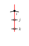
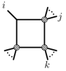
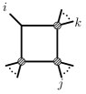
(a)	(b)	(c)

Figure 1: The twistor diagram shown in (a) depicts branch (16) of solutions to the three-mass box on-shell conditions $\langle\mathcal{L}\,i{-}1\,i\rangle=\langle\mathcal{L}\,i\,i{+}1\rangle=\langle\mathcal{L}\,j\,j{+}1\rangle=\langle\mathcal{L}\,k\,k{+}1\rangle=0$, which is a valid boundary for $\textrm{k}\geq 1$. This branch passes through the point $Z_{i}$ and intersects the lines $(j\,j{+}1)$ and $(k\,k{+}1)$. As drawn, the intersection at $j$ is an example of a non-MHV intersection, but the figure is agnostic about the relative cyclic ordering of $i,j,k$ and is intended to represent either possibility. Therefore, the corresponding Landau diagram can be either (b) or (c) depending on whether $i<j<k$ or $i<k<j$.

Although no such diagrams appear in this paper, the extension to higher loops is obvious: each $\mathcal{L}$ is represented by a line of a different color, and the presence of an on-shell condition of the form $\langle\mathcal{L}^{(\ell_{1})}\,\mathcal{L}^{(\ell_{2})}\rangle=0$ is indicated by an empty node at the intersection of the lines $\mathcal{L}^{(\ell_{1})}$ and $\mathcal{L}^{(\ell_{2})}$.

To each twistor diagram it is simple to associate one or more Landau diagrams, as also shown in Fig. 1. If a twistor diagram has a filled node at $i$ then an associated Landau diagram has two propagators $\langle\mathcal{L}\,i{-}1\,i\rangle$ and $\langle\mathcal{L}\,i\,i{+}1\rangle$ requiring a massless corner at $i$ in the Landau diagram. If a twistor diagram has an empty node on the line segment marked $i$ then an associated Landau diagram only has the single propagator $\langle\mathcal{L}\,i\,i{+}1\rangle$, requiring a massive corner in the Landau diagram. Therefore, twistor diagrams should be thought of as graphical shorthand which both depict the low-k solution to the cut conditions and simultaneously represent one or more Landau diagrams, as explained in the caption of Fig. 1.

One useful feature of this graphical notation is that the nodes of a twistor diagram fully encode the total number of propagators, $n_{\textrm{props}}$, in the Landau diagram (and so also the total number of on-shell conditions): each filled node accounts for two propagators, and each empty node accounts for one propagator:

$$n_{\textrm{props}}=2n_{\textrm{filled}}+n_{\textrm{empty}}\,.$$ (32)

This feature holds at higher loop order where this counting directly indicates how many propagators to associate with each loop.

Let us emphasize that a twistor diagram generally contains more information than its associated Landau diagram, as it indicates not only the set of on-shell conditions satisfied, but also specifies a particular branch of solutions thereto. The sole exception is the four-mass box, for which the above rules do not provide the twistor diagram with any way to distinguish the two branches (18), (19) of solutions. Moreover, the rules also do not provide any way to indicate that an $\mathcal{L}$ lies in a particular plane, such as $\overline{i}$. Therefore we can only meaningfully represent the low-k boundaries defined at the beginning of Sec. 5.

Given a twistor diagram depicting some branch, a twistor diagram corresponding to a relaxation of that branch may be obtained by deleting a non-MHV intersection of the type shown in (a) of Fig. 1, by replacing a filled node and its two line segments with an empty node and a single segment, or by deleting an empty node. In the associated Landau diagram, a relaxation corresponds to collapsing an internal edge of the graph. This is formalized in greater detail in Sec. 5.2.

5.2 A Graphical Recursion for Generating Low-helicity Boundaries

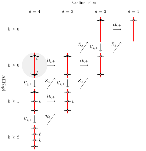
Figure 2: Twistor diagrams depicting eight types of low-k boundaries of $\textrm{N}^{\textrm{k}}\textrm{MHV}$ amplituhedra, organized according to the minimum value of k and the codimension $d$ (equivalently, the number of on-shell conditions satisfied). These correspond respectively to branch types (2), (1), (12), (7), (4), (16), (9) and (18)/(19). The graph operators $\mathcal{K}$, $\mathcal{R}$, and $\mathcal{U}$ are explained in the text and demonstrated in Figs. 3-5, respectively. Evidently all eight types of boundaries can be generated by acting with sequences of these operators on MHV maximal codimension boundaries of the type shown shaded in gray. There is an analogous parity-conjugated version of this hierarchy which relates all of the high-k branches to each other. The missing low-k boundary types (5), (6), (10), (11), (14) and (15) are degenerate cases which can be obtained by starting with $j=i+1$ in the gray blob.

In Fig. 2 we organize twistor diagrams representing eight types of boundaries according to $d$ and k; these are respectively the number of on-shell conditions $d$ satisfied on the boundary, and the minimum value of k for which the boundary is valid. It is evident from this data that there is a simple relation between $d$, k, and the number of filled ($n_{\textrm{filled}}$) and empty ($n_{\textrm{empty}}$) nodes. Specifically, we see that an $\textrm{N}^{\textrm{k}}\textrm{MHV}$ amplituhedron can have boundaries of a type displayed in a given twistor diagram only if

$$\textrm{k}\geq 2n_{\textrm{empty}}+3n_{\textrm{filled}}-d-2=n_{\textrm{empty}}+n_{\textrm{filled}}-2\,,$$ (33)

where we have used Eq. (32) with $n_{\textrm{props}}=d$. In the sequel we will describe a useful map from Landau diagrams to the on-shell diagrams of ArkaniHamed:2012nw which manifests the relation (33) and provides a powerful generalization thereof to higher loop order. The amplituhedron-based approach has some advantages over that of enumerating on-shell diagrams that will also be explored in the sequel. First of all, the minimal required helicity of a multi-loop configuration can be read off from each loop line separately. Second, we immediately know the relevant solution branches for a given helicity. And finally, compared to enumerating all relevant on-shell diagrams the amplituhedron-based method is significantly more compact since it can be used to produce a minimal subset of diagrams such that all allowed diagrams are relaxations thereof, including limits where massive external legs become massless or vanish.

From the data displayed in Fig. 2 we see that a natural organizational principle emerges: all $\textrm{N}^{\textrm{k}}\textrm{MHV}$ one-loop twistor diagrams can be obtained from the unique maximal codimension MHV diagram (shown shaded in gray) via sequences of simple graph operations which we explain in turn.

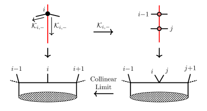
Figure 3: The graph operation $\mathcal{K}_{i}$ maps an $\textrm{N}^{\textrm{k}}\textrm{MHV}$ twistor diagram into an $\textrm{N}^{\textrm{k}+1}\textrm{MHV}$ twistor diagram as shown in the top row. On Landau diagrams, this corresponds to replacing a massless corner by a massive corner; such an operation is effectively an inverse collinear limit. The shaded region in the figures represents an arbitrary planar sub-graph. A dashed external line on a Landau diagram may be either one massless external leg so the whole corner is massive, or completely removed so the whole corner is massless.

The first graph operation $\mathcal{K}$ increments the helicity of the diagram on which it operates. (The name $\mathcal{K}$ is a reminder that it increases k.) Its operation is demonstrated in Fig. 3. Specifically, $\mathcal{K}_{i}$ replaces a filled node at a point $i$ along $\mathcal{L}$ by two empty nodes, one at $i$ and a second one on a new non-MHV intersection added to the diagram. Since $n_{\textrm{filled}}$ decreases by one but $n_{\textrm{empty}}$ increases by two under this operation, it is clear from Eq. (33) that $\mathcal{K}_{i}$ always increases by one the minimal value of k on which the branch indicated by the twistor diagram has support. From the point of view of Landau diagrams, this operation replaces a massless node with a massive one, as illustrated in the bottom row of Fig. 3, and hence it may be viewed as an “inverse” collinear limit.

The other two graph operations $\mathcal{R}$ and $\mathcal{U}$ both correspond to relaxations, as defined in Sec. 2.3, since they each reduce the number of on-shell conditions by one, stepping thereby one column to the right in Fig. 2.

The operation $\mathcal{R}_{i}$ simply removes (hence the name $\mathcal{R}$) an empty node $i$ from a twistor diagram, as shown in Fig. 4. This corresponds to removing $\langle\mathcal{L}\,i\,i+1\rangle=0$ from the set of on-shell conditions satisfied by $\mathcal{L}$.

The last operation, $\mathcal{U}$, corresponds to “un-pinning” a filled node (hence “$\mathcal{U}$”). Un-pinning means removing one constraint from a pair $\langle\mathcal{L}\,i{-}1\,i\rangle=\langle\mathcal{L}\,i\,i{+}1\rangle=0$. The line $\mathcal{L}$, which was pinned to the point $i$, is then free to slide along the line segment $(i{-}1\,i)$ or $(i\,i{+}1)$ (for $\mathcal{U}_{i,-}$ or $\mathcal{U}_{i,+}$, respectively). In the twistor diagram, this is depicted by replacing the filled node at the point $i$ with a single empty node along the line segment $(i\,i{\pm}1)$ (see Fig. 5). Only $\mathcal{U}_{+}$ appears in Fig. 2 because at one loop, all diagrams generated by any $\mathcal{U}_{-}$ operation are equivalent, up to relabeling, to some diagram generated by a $\mathcal{U}_{+}$. In general, however, it is necessary to track the subscript $\pm$ since both choices are equally valid relaxations and can yield inequivalent twistor and Landau diagrams. From Fig. 2, we read off the following identity among the operators acting on any diagram $g$:

$$\mathcal{U}_{j,+}g=\mathcal{R}_{k}\mathcal{K}_{j,+}g\,.$$ (34)

There was no reason to expect the simple graphical pattern of Fig. 5 to emerge among the twistor diagrams. Indeed in Sec. 3 we simply listed all possible sets of on-shell conditions without taking such an organizational principle into account. At higher loop order, however, the problem of enumerating all boundaries of $\textrm{N}^{\textrm{k}}\textrm{MHV}$ amplituhedra benefits greatly from the fact that all valid configurations of each single loop can be iteratively generated via these simple rules, starting from the maximal codimension MHV boundaries. Stated somewhat more abstractly, these graph operations are instructions for naturally associating boundaries of different amplituhedra.

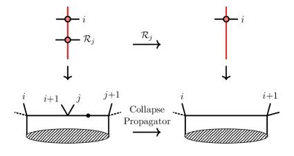
Figure 4: The graph operation $\mathcal{R}_{j}$ relaxes $\mathcal{L}$ by removing the condition that $\mathcal{L}$ must pass through the line $(j\,j{+}1)$; this is equivalent to removing the on-shell condition $\langle\mathcal{L}\,j\,j{+}1\rangle=0$. On Landau diagrams, this corresponds to collapsing the propagator indicated by the filled dot in the bottom figure on the left. The shaded region in the figures represents an arbitrary planar sub-graph. A dashed external line on a Landau diagram may be either one massless external leg so the whole corner is massive, or completely removed so the whole corner is massless. It is to be understood that the graphical notation implies that $j\neq i+2$ and $i\neq j+2$; otherwise, the two empty nodes in the top left diagram would be represented by a single filled node on which the action of $\mathcal{R}$ is undefined; the appropriate graph operation in this case would instead be $\mathcal{U}$.

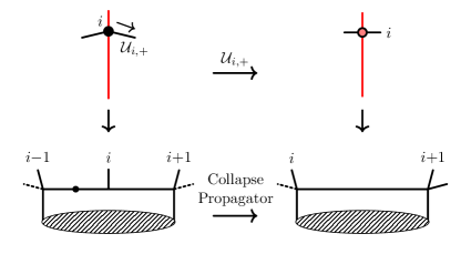
Figure 5: The graph operation $\mathcal{U}_{i,+}$ relaxes a line $\mathcal{L}$ constrained to pass through the point $i$, shifting it to lie only along the line $(i\,i{+}1)$. This is equivalent to removing the on-shell constraint $\langle\mathcal{L}\,i{-}1\,i\rangle=0$. (The equally valid relaxation $\mathcal{U}_{i,-}$, not pictured here, lets the intersection point slide onto $(i{-}1\,i)$.) On Landau diagrams, this corresponds to collapsing the propagator indicated by the filled dot in the bottom figure on the left. The shaded region in the figures represents an arbitrary planar sub-graph. A dashed external line on a Landau diagram may be either one massless external leg so the whole corner is massive, or completely removed so the whole corner is massless. As explained in the caption of Fig. 4, the $\mathcal{U}$ operation can be thought of as a special case of the $\mathcal{R}$ operation, and we distinguish the two because only the latter can change the helicity sector k.

Before concluding this section it is worth noting (as is evident in Fig. 2) that relaxing a low-k boundary can never raise the minimum value of k for which that type of boundary is valid. In other words, we find that if $\mathcal{A}_{n,\textrm{k},1}$ has a boundary of type $B$, and if $B^{\prime}$ is a relaxation of $B$, then $\mathcal{A}_{n,\textrm{k},1}$ also has boundaries of type $B^{\prime}$. This property does not hold in general beyond one loop; a counterexample involving two-loop MHV amplitudes appears in Fig. 4 of Dennen:2016mdk .

6 Solving Landau Equations in Momentum Twistor Space

As emphasized in Sec. 2.5, the Landau equations naturally associate to each boundary of an amplituhedron a locus in $\operatorname{Conf}_{n}(\mathbb{P}^{3})$ on which the corresponding amplitude has a singularity. In this section we review the results of solving the Landau equations for each of the one-loop branches classified in Sec. 3, thereby carrying out step 2 of the algorithm summarized in Sec. 2.5. The results of this section were already tabulated in Dennen:2015bet , but we revisit the analysis, choosing just two examples, in order to demonstrate the simplicity and efficiency of these calculations when carried out directly in momentum twistor space. The utility of this method is on better display in the higher-loop examples to be considered in the sequel.

As a first example, we consider the tadpole on-shell condition

$$f_{1}\equiv\langle\mathcal{L}\,i\,i{+}1\rangle=0\,.$$ (35)

We choose any two other points $Z_{j}$, $Z_{k}$ (which generically satisfy $\langle i\,i{+}1\,j\,k\rangle\neq 0$) in terms of which to parameterize

$$\mathcal{L}=(Z_{i}+d_{1}Z_{j}+d_{2}Z_{k},Z_{i+1}+d_{3}Z_{j}+d_{4}Z_{k})\,.$$ (36)

Then the on-shell condition (35) admits solutions when

$$d_{1}d_{4}-d_{2}d_{3}=0\,,$$ (37)

while the four Kirchhoff conditions (10) are

$$\alpha_{1}d_{4}=-\alpha_{1}d_{3}=-\alpha_{1}d_{2}=\alpha_{1}d_{1}=0\,.$$ (38)

The only nontrivial solution (that means $\alpha_{1}\neq 0$; see Sec. 2.4) to the equations (37) and (38) is to set all four $d_{A}=0$. Since this solution exists for all (generic) projected external data, it does not correspond to a branch point of an amplitude and is uninteresting to us. In other words, in this case the locus we associate to a boundary of this type is all of $\operatorname{Conf}_{n}(\mathbb{P}^{3})$.

As a second example, consider the two on-shell conditions corresponding to the two-mass bubble

$$f_{1}\equiv\langle\mathcal{L}\,i\,i{+}1\rangle=0\,,\qquad f_{2}\equiv\langle\mathcal{L}\,j\,j{+}1\rangle=0\,.$$ (39)

In this case a convenient parameterization is

$$\mathcal{L}=(Z_{i}+d_{1}Z_{i+1}+d_{2}Z_{k},Z_{j}+d_{3}Z_{i+1}+d_{4}Z_{k})\,.$$ (40)

Note that an asymmetry between $i$ and $j$ is necessarily introduced because we should not allow more than four distinct momentum twistors to appear in the parameterization, since they would necessarily be linearly dependent, and we assume of course that $Z_{k}$ is generic (meaning, as before, that $\langle i\,i{+}1\,j\,k\rangle\neq 0$). Then

$$f_{1} =-d_{2}\langle i\,i{+}1\,j\,k\rangle\,,$$ (41)

$$f_{2} =d_{3}\langle i\,i{+}1\,j\,j{+}1\rangle+d_{4}\langle i\,j\,j{+}1\,k\rangle+(d_{1}d_{4}-d_{2}d_{3})\langle i{+}1\,j\,j{+}1\,k\rangle$$ (42)

and the Kirchhoff conditions are

$$\left(\begin{matrix}0&d_{4}\langle i{+}1\,j\,j{+}1\,k\rangle\\ -\langle i\,i{+}1\,j\,k\rangle&-d_{3}\langle i{+}1\,j\,j{+}1\,k\rangle\\ 0&\langle i\,i{+}1\,j\,j{+}1\rangle-d_{2}\langle i{+}1\,j\,j{+}1\,k\rangle\\ 0&\langle i\,j\,j{+}1\,k\rangle+d_{1}\langle i{+}1\,j\,j{+}1\,k\rangle\end{matrix}\right)\left(\begin{matrix}\alpha_{1}\\ \alpha_{2}\end{matrix}\right)=0\,.$$ (43)

Nontrivial solutions exist only if all $2\times 2$ minors of the $4\times 2$ coefficient matrix vanish. Three minors are trivially zero, and the one computed from the second and third rows evaluates simply to

$$-\langle i\,i{+}1\,j\,k\rangle\langle i\,i{+}1\,j\,j{+}1\rangle=0$$ (44)

using the on-shell condition $f_{1}=-d_{2}\langle i\,i{+}1\,j\,k\rangle=0$. If this quantity vanishes, then the four remaining constraints (the two on-shell conditions $f_{1}=f_{2}=0$ and the two remaining minors) can be solved for the four $d_{A}$, and then Eq. (43) can be solved to find the two $\alpha_{J}$’s. Since $\langle i\,i{+}1\,j\,k\rangle\neq 0$ by assumption, we conclude that the Landau equations admit nontrivial solutions only on the codimension-one locus in $\operatorname{Conf}_{n}(\mathbb{P}^{3})$ where

$$\langle i\,i{+}1\,j\,j{+}1\rangle=0\,.$$ (45)

These two examples demonstrate that in some cases (e.g. the tadpole example) the Landau equations admit solutions for any (projected) external data, while in other cases (e.g. the bubble example) the Landau equations admit solutions only when there is a codimension-one constraint on the external data. A common feature of these examples is that some care must be taken in choosing how to parameterize $\mathcal{L}$. In particular, one must never express $\mathcal{L}$ in terms of four momentum twistors ($Z_{i}$, $Z_{j}$, etc.) that appear in the specification of the on-shell conditions; otherwise, it can be impossible to disentangle the competing requirements that these satisfy some genericity (such as $\langle i\,i{+}1\,j\,k\rangle\neq 0$ in the above examples) while simultaneously hoping to tease out the constraints they must satisfy in order to have a solution (such as Eq. (45)). For example, although one might have been tempted to preserve the symmetry between $i$ and $j$, it would have been a mistake to use the four twistors $Z_{i}$, $Z_{i+1}$, $Z_{j}$ and $Z_{j+1}$ in Eq. (40).

Instead, it is safest to always pick four completely generic points $Z_{a},\ldots,Z_{d}$ in terms of which to parameterize

$$\mathcal{L}=\left(\begin{matrix}1&0&d_{1}&d_{2}\cr 0&1&d_{3}&d_{4}\end{matrix}\right)\left(\begin{matrix}Z_{a}\cr Z_{b}\cr Z_{c}\cr Z_{d}\end{matrix}\right).$$ (46)

The disadvantage of being so careful is that intermediate steps in the calculation become much more lengthy, a problem we avoid in practice by using a computer algebra system such as Mathematica.

The results of this analysis for all one-loop branches are summarized in Tab. LABEL:tab:bigtable. Naturally these are in accord with those of Landau:1959fi (as tabulated in Dennen:2015bet ). At one loop it happens that the singularity locus is the same for each branch of solutions to a given set of on-shell conditions, but this is not generally true at higher loop order.

7 Singularities and Symbology

As suggested in the introduction (and explicit even in the title of this paper), one of the goals of our research program is to provide a priori derivations of the symbol alphabets of various amplitudes. We refer the reader to Goncharov:2010jf for more details, pausing only to recall that the symbol alphabet of a generalized polylogarithm function $F$ is a finite list of symbol letters $\{z_{1},\ldots,z_{r}\}$ such that $F$ has logarithmic branch cuts (i.e., the cover has infinitely many sheets) between $z_{i}=0$ and $z_{i}=\infty$ for each $i=1,\ldots,r$.

To date, symbol alphabets have been determined by explicit computation only for two-loop MHV amplitudes CaronHuot:2011ky ; all other results on multi-loop SYM amplitudes in the literature are based on a conjectured extrapolation of these results to higher loop order. Throughout the paper we have however been careful to phrase our results in terms of branch points, rather than symbol letters, for two reasons.

First of all, amplitudes in SYM theory are expected to be expressible as generalized polylogarithm functions, with symbol letters that have a familiar structure like those of the entries in the last column of Tab. LABEL:tab:bigtable, only for sufficiently low (or, by parity conjugation, high) helicity. In contrast, the Landau equations are capable of detecting branch points of even more complicated amplitudes, such as those containing elliptic polylogarithms, which do not have traditional symbols.

Second, even for amplitudes which do have symbols, determining the actual symbol alphabet from the singularity loci of the amplitude may require nontrivial extrapolation. Suppose that the Landau equations reveal that some amplitude has a branch point at $z=0$ (where, for example, $z$ may be one of the quantities in the last column of Tab. LABEL:tab:bigtable). Then the symbol alphabet should contain a letter $f(z)$, where $f$ in general could be an arbitrary function of $z$, with branch points arising in two possible ways. If $f(0)=0$, then the amplitude will have a logarithmic branch point at $z=0$ Maldacena:2015iua , but even if $f(0)\neq 0$, the amplitude can have an algebraic branch point (so the cover has finitely many sheets) at $z=0$ if $f(z)$ has such a branch point there.

We can explore this second notion empirically since all one-loop amplitudes in SYM theory, and in particular their symbol alphabets, are well-known (following from one-loop integrated amplitudes in for example, tHooft:1978jhc ; Bern:1993kr ; Bern:1994zx ; Bern:1994ju ; Brandhuber:2004yw ; Bern:2004ky ; Britto:2004nc ; Bern:2004bt ; Ellis:2007qk ). According to our results from Tab. LABEL:tab:bigtable, we find that one-loop amplitudes only have branch points on loci of the form

• $\langle i\,i{+}1\,j\,j{+}1\rangle=0$ or $\langle i\,\overline{j}\rangle=0$ for $0\leq\textrm{k}\leq n-4$,

• $\langle i(i{-}1\,i{+}1)(j\,j{+}1)(k\,k{+}1)\rangle=0$ for $1\leq\textrm{k}\leq n-5$, and

• $\Delta_{ijk\ell}=0$ (defined in Tab. LABEL:tab:bigtable) for $2\leq\textrm{k}\leq n-6$,

where $i,j,k,\ell$ can all range from $1$ to $n$. Happily, the first two of these are in complete accord with the symbol letters of one-loop MHV and NMHV amplitudes, but the third reveals the foreshadowed algebraic branching since $\Delta_{ijk\ell}$ is not a symbol letter of the four-mass box integral contribution to $\textrm{N}^{2\leq\textrm{k}\leq n-6}\textrm{MHV}$ amplitudes. Rather, the symbol alphabet of this amplitude consists of quantities of the form

$$f_{ij}\equiv\langle i\,i{+}1\,j\,j{+}1\rangle\quad\textrm{and}\quad f_{i\ell}f_{jk}\pm(f_{ik}f_{j\ell}-f_{ij}f_{k\ell})\pm\sqrt{\Delta_{ijk\ell}}\,,$$ (47)

where the signs may be chosen independently. Since no symbol letter vanishes on the locus $\Delta_{ijk\ell}=0$, amplitudes evidently do not have logarithmic branch points on this locus. Yet it is evident from the second expression of (47) that amplitudes with these letters have algebraic (in this instance, square-root- or double-sheet-type) branch points when $\Delta_{ijk\ell}=0$.

Although we have only commented on the structure of various potential symbol entries and branch point loci here, let us emphasize that the methods of this paper can be used to determine precisely which symbol entries can appear in any given amplitude. For example, Tab. LABEL:tab:bigtable can be used to determine values of $i$, $j$ and $k$ for which the letter $\langle i(i{-}1\,i{+}1)(j\,j{+}1)(k\,k{+}1)\rangle$ can appear, as well as in which one-loop amplitudes, indexed by $n$ and $k$, such letters will appear. An example of a fine detail along these lines evident already in Tab. LABEL:tab:bigtable is the fact that all NMHV amplitudes have branch points of two-mass easy type except for the special case $n=6$, in accord with Eq. (2.7) of Kosower:2010yk .

We conclude this section by remarking that the problem of deriving symbol alphabets from the Landau singularity loci may remain complicated in general, but we hope that the simple, direct correspondence we have observed for certain one-loop amplitudes (and which was also observed for the two-loop MHV amplitudes studied in Dennen:2016mdk ) will continue to hold at arbitrary loop order for sufficiently simple singularities.

8 Conclusion

This paper presents first steps down the path of understanding the branch cut structure of SYM amplitudes for general helicity, following the lead of Dennen:2016mdk and using the recent “unwound” formulation of the amplituhedron from Arkani-Hamed:2017vfh . Our algorithm is conceptually simple: we first enumerate the boundaries of an amplituhedron, and from there, without resorting to integral representations, we use the Landau equations directly to determine the locations of branch points of the corresponding amplitude.

One might worry that each of these steps grows rapidly in computational complexity at higher loop order. Classifying boundaries of amplituhedra is on its own a highly nontrivial problem, aspects of which have been explored in Arkani-Hamed:2013kca ; Franco:2014csa ; Bai:2015qoa ; Galloni:2016iuj ; Karp:2017ouj . In that light, the graphical tools presented in Sec. 5.2, while already useful for organizing results as in Fig. 2, hint at the more enticing possibility of a method to enumerate twistor diagrams corresponding to all $\mathcal{L}$-boundaries of any given $\mathcal{A}_{n,\textrm{k},L}$. Such an algorithm would start with the maximal codimension twistor diagrams at a given loop order, and apply the operators of Sec. 5.2 in all ways until no further operations are possible. From these twistor diagrams come Landau diagrams, and from these come the branch points via the Landau equations. We saw in Dennen:2016mdk and Sec. 6 that analyzing the Landau equations can be made very simple in momentum twistor space.

Configurations of loop momenta in (the closure of) MHV amplituhedra are represented by non-negative $D$-matrices. In general, non-MHV configurations must be represented by indefinite $D$-matrices, but we observed in Sec. 4.5 that even for non-MHV amplituhedra, $D$ may always be chosen non-negative for all configurations on $\mathcal{L}$-boundaries. This ‘emergent positivity’ plays a crucial role by allowing the one-loop $D$-matrices presented in Secs. 4.2, 4.3 and 4.4 to be trivially recycled at higher values of helicity. One way to think about this is to say that going beyond MHV level introduces the $C$-matrix which “opens up” additional configuration space in which an otherwise indefinite $D$-matrix can become positive.

While the one-loop all-helicity results we obtain are interesting in their own right as first instances of all-helicity statements, this collection of information is valuable because it provides the building blocks for the two-loop analysis in the sequel. There we will argue that the two-loop twistor diagrams with helicity k can be viewed as compositions of two one-loop diagrams with helicities $\textrm{k}_{1}$ and $\textrm{k}_{2}$ satisfying $\textrm{k}=\textrm{k}_{1}+\textrm{k}_{2}$ or $\textrm{k}_{1}+\textrm{k}_{2}+1$. We will also explore in detail the relation to on-shell diagrams, which are simply Landau diagrams with decorated nodes.

More speculatively, the ideas that higher-loop amplitudes can be constructed from lower-loop amplitudes, and that there is a close relation to on-shell diagrams, suggests the possibility that this toolbox may also be useful for finding symbols in the full, nonplanar SYM theory. For example, enumerating the on-shell conditions as we do here in the planar sector is similar in spirit to the nonplanar examples of Bern:2015ple where certain integral representations were found such that individual integrals had support on only certain branches. There are of course far fewer known results in the nonplanar SYM theory, though there have been some preliminary studies Arkani-Hamed:2014via ; Bern:2014kca ; Bern:2017gdk ; Franco:2015rma ; Bourjaily:2016mnp .

- (1) L. Brink, J. H. Schwarz and J. Scherk, Nucl. Phys. B 121, 77 (1977).
- (2) T. Dennen, M. Spradlin and A. Volovich, JHEP 1603, 069 (2016) [arXiv:1512.07909 [hep-th]].
- (3) T. Dennen, I. Prlina, M. Spradlin, S. Stanojevic and A. Volovich, JHEP 1706, 152 (2017) [arXiv:1612.02708 [hep-th]].
- (4) N. Arkani-Hamed, J. L. Bourjaily, F. Cachazo, A. B. Goncharov, A. Postnikov and J. Trnka, arXiv:1212.5605 [hep-th].
- (5) J. Golden, A. B. Goncharov, M. Spradlin, C. Vergu and A. Volovich, JHEP 1401, 091 (2014) [arXiv:1305.1617 [hep-th]].
- (6) J. Golden and M. Spradlin, JHEP 1502, 002 (2015) [arXiv:1411.3289 [hep-th]].
- (7) J. Drummond, J. Foster and O. Gurdogan, Phys. Rev. Lett. 120, no. 16, 161601 (2018) [arXiv:1710.10953 [hep-th]].
- (8) L. J. Dixon, J. M. Drummond, C. Duhr, M. von Hippel and J. Pennington, PoS LL 2014, 077 (2014) [arXiv:1407.4724 [hep-th]].
- (9) S. Caron-Huot, L. J. Dixon, A. McLeod and M. von Hippel, Phys. Rev. Lett. 117, no. 24, 241601 (2016) [arXiv:1609.00669 [hep-th]].
- (10) J. M. Drummond, G. Papathanasiou and M. Spradlin, JHEP 1503, 072 (2015) [arXiv:1412.3763 [hep-th]].
- (11) L. J. Dixon, J. Drummond, T. Harrington, A. J. McLeod, G. Papathanasiou and M. Spradlin, JHEP 1702, 137 (2017) [arXiv:1612.08976 [hep-th]].
- (12) R. E. Cutkosky, J. Math. Phys. 1, 429 (1960).
- (13) R. J. Eden, P. V. Landshoff, D. I. Olive and J. C. Polkinghorne, Cambridge University Press, 1966.
- (14) L. D. Landau, Nucl. Phys. 13, 181 (1959).
- (15) Z. Bern, L. J. Dixon, D. C. Dunbar and D. A. Kosower, Nucl. Phys. B 435, 59 (1995) [hep-ph/9409265].
- (16) F. Cachazo, P. Svrcek and E. Witten, JHEP 0409, 006 (2004) [hep-th/0403047].
- (17) R. Britto, F. Cachazo, B. Feng and E. Witten, Phys. Rev. Lett. 94, 181602 (2005) [hep-th/0501052].
- (18) H. Elvang and Y. t. Huang, arXiv:1308.1697 [hep-th].
- (19) N. Arkani-Hamed and J. Trnka, JHEP 1410, 030 (2014) [arXiv:1312.2007 [hep-th]].
- (20) N. Arkani-Hamed, H. Thomas and J. Trnka, JHEP 1801, 016 (2018) [arXiv:1704.05069 [hep-th]].
- (21) G. ’t Hooft and M. J. G. Veltman, Nucl. Phys. B 153, 365 (1979).
- (22) Z. Bern, L. J. Dixon and D. A. Kosower, Nucl. Phys. B 412, 751 (1994) [hep-ph/9306240].
- (23) Z. Bern, L. J. Dixon, D. C. Dunbar and D. A. Kosower, Nucl. Phys. B 425, 217 (1994) [hep-ph/9403226].
- (24) Z. Bern, L. J. Dixon, D. C. Dunbar and D. A. Kosower, In *Minneapolis 1994, Proceedings, Continuous advances in QCD* 3-21, and SLAC Stanford - SLAC-PUB-6490 (94,rec.May) 23 p. Saclay CEN - S.PH.T-94-055 (94,rec.May) 23 p. Calif. U. Los Angeles - UCLA-94-TEP-17 (94,rec.May) 23 p [hep-ph/9405248].
- (25) A. Brandhuber, B. J. Spence and G. Travaglini, Nucl. Phys. B 706, 150 (2005) [hep-th/0407214].
- (26) Z. Bern, V. Del Duca, L. J. Dixon and D. A. Kosower, Phys. Rev. D 71, 045006 (2005) [hep-th/0410224].
- (27) R. Britto, F. Cachazo and B. Feng, Nucl. Phys. B 725, 275 (2005) [hep-th/0412103].
- (28) Z. Bern, L. J. Dixon and D. A. Kosower, Phys. Rev. D 72, 045014 (2005) [hep-th/0412210].
- (29) R. K. Ellis and G. Zanderighi, JHEP 0802, 002 (2008) [arXiv:0712.1851 [hep-ph]].
- (30) I. Prlina, M. Spradlin, J. Stankowicz and S. Stanojevic, arXiv:1712.08049 [hep-th].
- (31) A. Hodges, JHEP 1305, 135 (2013) [arXiv:0905.1473 [hep-th]].
- (32) S. J. Parke and T. R. Taylor, Phys. Rev. Lett. 56, 2459 (1986).
- (33) V. P. Nair, Phys. Lett. B 214, 215 (1988).
- (34) Z. Bern, L. J. Dixon and V. A. Smirnov, Phys. Rev. D 72, 085001 (2005) [hep-th/0505205].
- (35) L. F. Alday, D. Gaiotto and J. Maldacena, JHEP 1109, 032 (2011) [arXiv:0911.4708 [hep-th]].
- (36) J. M. Drummond, J. Henn, G. P. Korchemsky and E. Sokatchev, Nucl. Phys. B 828, 317 (2010) [arXiv:0807.1095 [hep-th]].
- (37) G. F. Sterman and M. E. Tejeda-Yeomans, Phys. Lett. B 552, 48 (2003) [hep-ph/0210130].
- (38) Y. Bai, S. He and T. Lam, JHEP 1601, 112 (2016) [arXiv:1510.03553 [hep-th]].
- (39) N. Arkani-Hamed, J. L. Bourjaily, F. Cachazo and J. Trnka, JHEP 1206, 125 (2012) [arXiv:1012.6032 [hep-th]].
- (40) J. L. Bourjaily, S. Caron-Huot and J. Trnka, JHEP 1501, 001 (2015) [arXiv:1303.4734 [hep-th]].
- (41) A. P. Hodges, hep-th/0503060.
- (42) A. B. Goncharov, M. Spradlin, C. Vergu and A. Volovich, Phys. Rev. Lett. 105, 151605 (2010) [arXiv:1006.5703 [hep-th]].
- (43) S. Caron-Huot, JHEP 1112, 066 (2011) [arXiv:1105.5606 [hep-th]].
- (44) J. Maldacena, D. Simmons-Duffin and A. Zhiboedov, JHEP 1701, 013 (2017) [arXiv:1509.03612 [hep-th]].
- (45) D. A. Kosower, R. Roiban and C. Vergu, Phys. Rev. D 83, 065018 (2011) [arXiv:1009.1376 [hep-th]].
- (46) N. Arkani-Hamed and J. Trnka, JHEP 1412, 182 (2014) [arXiv:1312.7878 [hep-th]].
- (47) S. Franco, D. Galloni, A. Mariotti and J. Trnka, JHEP 1503, 128 (2015) [arXiv:1408.3410 [hep-th]].
- (48) D. Galloni, arXiv:1601.02639 [hep-th].
- (49) S. N. Karp, L. K. Williams and Y. X. Zhang, arXiv:1708.09525 [math.CO].
- (50) Z. Bern, E. Herrmann, S. Litsey, J. Stankowicz and J. Trnka, JHEP 1606, 098 (2016) [arXiv:1512.08591 [hep-th]].
- (51) J. L. Bourjaily, E. Herrmann and J. Trnka, JHEP 1706, 059 (2017) [arXiv:1704.05460 [hep-th]].
- (52) Z. Bern, E. Herrmann, S. Litsey, J. Stankowicz and J. Trnka, JHEP 1506, 202 (2015) [arXiv:1412.8584 [hep-th]].
- (53) N. Arkani-Hamed, J. L. Bourjaily, F. Cachazo and J. Trnka, Phys. Rev. Lett. 113, no. 26, 261603 (2014) [arXiv:1410.0354 [hep-th]].
- (54) Z. Bern, M. Enciso, H. Ita and M. Zeng, Phys. Rev. D 96, no. 9, 096017 (2017) [arXiv:1709.06055 [hep-th]].
- (55) J. L. Bourjaily, S. Franco, D. Galloni and C. Wen, JHEP 1610, 003 (2016) [arXiv:1607.01781 [hep-th]].
- (56) S. Franco, D. Galloni, B. Penante and C. Wen, JHEP 1506, 199 (2015) [arXiv:1502.02034 [hep-th]].