Freezing In, Heating Up, and Freezing Out:
Predictive Nonthermal Dark Matter and Low-Mass Direct Detection

Abstract

Freeze-in dark matter (DM) mediated by a light ($\ll$ keV) weakly-coupled dark-photon is an important benchmark for the emerging low-mass direct detection program. Since this is one of the only predictive, detectable freeze-in models, we investigate how robustly such testability extends to other scenarios. For concreteness, we perform a detailed study of models in which DM couples to a light scalar mediator and acquires a freeze-in abundance through Higgs-mediator mixing. Unlike dark-photons, whose thermal properties weaken stellar cooling bounds, the scalar coupling to Standard Model (SM) particles is subject to strong astrophysical constraints, which severely limit the fraction of DM that can be produced via freeze-in. While it seems naively possible to compensate for this reduction by increasing the mediator-DM coupling, sufficiently large values eventually thermalize the dark sector with itself and yield efficient DM annihilation to mediators, which depletes the freeze-in population; only a small window of DM candidate masses near the $\sim$ GeV scale can accommodate the total observed abundance. Since many qualitatively similar issues arise for other light mediators, we find it generically difficult to realize a viable freeze-in scenario in which production arises only from renormalizable interactions with SM particles. We also comment on several model variations that may evade these conclusions.

1 Introduction

Despite overwhelming evidence demonstrating the existence of dark matter (DM) on galactic and cosmological scales Bertone:2016nfn , identifying its possible non-gravitational interactions remains one of the greatest challenges in contemporary physics. Historically, much of the DM search program has been guided by the weakly interacting massive particle (WIMP) hypothesis in which $\sim$ TeV-scale DM carries electroweak charge and acquires its abundance by freezing out of equilibrium from the Standard Model (SM). However, decades of null searches Roszkowski:2017nbc have motivated a new, broader paradigm in which DM is the lightest stable SM singlet in a “hidden sector” with its own dynamics and cosmological history (see Alexander:2016aln ; Battaglieri:2017aum for a review). In these scenarios the viable DM mass range can span many orders of magnitude, so there is strong motivation for new detection techniques.

Recently, there has been great progress in proposing new direct-detection targets for the $\sim$ keV–GeV DM mass range. Some representative ideas involve scattering off atomic electrons Essig:2011nj ; Essig:2012yx ; Essig:2017kqs , superconductors Hochberg:2015pha ; Hochberg:2016ajh , semiconductors Essig:2011nj ; Graham:2012su ; Tiffenberg:2017aac ; Essig:2015cda , Helium evaporation Maris:2017xvi , Fermi-degenerate materials Hochberg:2015fth , Dirac metals Hochberg:2017wce , Graphene targets Hochberg:2016ntt , magnetic bubble chambers Bunting:2017net , color centers Budnik:2017sbu , and chemical bonds Essig:2016crl (for a review, see Battaglieri:2017aum ). Unlike traditional direct detection experiments, designed for WIMP scattering off heavy nuclei with $\sim$ recoil energy thresholds, many of these techniques exploit observable transitions between small internal energy levels (e.g. atomic ionization) to probe much lighter DM, which typically deposits $\sim-{\rm few}\,$ per scatter. Furthermore, these targets are particularly sensitive to interactions mediated by light particles $\phi$ whose recoil spectra are sharply peaked towards low recoil energies, so the scattering cross section can be greatly enhanced

$$\sigma_{e}\sim\frac{g_{\chi}^{2}g_{e}^{2}m^{2}_{e}}{(q^{2}+m_{\phi}^{2})^{2}}~{}\longrightarrow~{}\frac{g^{2}_{\chi}g_{e}^{2}}{q^{4}}\sim 5\times 10^{-38}\,{}^{2}\biggl{(}\frac{g_{\chi}^{2}g_{e}^{2}}{10^{-25}}\biggr{)}\left(\frac{\alpha m_{e}}{q}\right)^{4},$$ (1)

and may be observable even for extremely small couplings. Here $g_{\chi/f}$ are the $\phi$ couplings to dark/visible particles where $f$ is a SM fermion and, for illustration, we have taken $m_{\chi}\gtrsim m_{e}$ and normalized to the characteristic momentum transfer $q\sim\alpha m_{e}$ for DM scattering off atomic electrons Essig:2011nj . However, if $g_{f}$ is sufficiently large to thermalize $\phi$ with the SM in the early universe, cosmological bounds from BBN and $\Delta N_{\rm eff}$ generically require $m_{\phi}\gtrsim$ MeV Pospelov:2010hj , which is outside the range in which Eq. (1) holds. Thus, in order to exploit this huge enhancement, we demand $g_{f}\ll 1$ to avoid thermalizing with the photons, which excludes thermal DM production with a sub-MeV mediator, but still allows for non-equilibrium alternatives.

Aside from thermal freeze-out, the only other predictive, UV insensitive production mechanism is “freeze-in” McDonald:2001vt ; Hall:2009bx , in which DM is not initially populated during reheating, but produced later through sub-Hubble interactions with SM particles. Since DM never achieves a thermal number density, its Boltzmann equation is integrable and the final abundance is

$$~{}~{}~{}~{}\Omega_{\chi}\simeq\frac{m_{\chi}s_{0}}{\rho_{\rm cr}}\int_{\infty}^{m_{\chi}}\frac{dT}{T}\frac{n^{2}_{\rm\small SM}}{Hs}\langle\sigma v_{{\rm SM}\to\chi\chi}\rangle~{}~{}~{}~{}~{}(\rm traditional~{}freeze~{}in),$$ (2)

where $T$ is the SM temperature, $H$ is the Hubble expansion rate, $s$ is the entropy density, $\rho_{\rm cr}$ is the critical density, $n_{\rm SM}$ is the number density for some SM species, and a $0$ subscript represents a present day value. As with freeze-out, the abundance is fixed by the DM-SM interaction and is insensitive to the details of earlier, unknown cosmological epochs (e.g. inflation, reheating). Although the couplings required for freeze-in production are generically very small for light mediators, it may nonetheless be possible to exploit the low thresholds of these experiments to bring the cross section in Eq. (1) into the observable range.

It has been shown that many new direct-detection targets are potentially sensitive to the freeze-in parameter space for DM with interactions mediated by an ultra-light ($\ll$) dark-photon Chu:2011be ; Essig:2015cda . However, this particular model has many special features, which do not generalize to other mediators (or even to heavier dark-photons). Most notably, the in-medium thermal suppression of kinetic mixing at finite temperature counterintuitively makes the nearly-massless dark-photon safer from astrophysical and cosmological bounds because all on-shell production vanishes in the massless mediator limit Chang:2016ntp ; Hardy:2016kme . Furthermore, in this limit, the cosmological dark-photon production is also suppressed, so it can be neglected in the Boltzmann system and Eq. (2) can be straightforwardly applied. However, in models for which mediator production is not parametrically suppressed in the early universe, Eq. (2) is no longer valid and it is necessary to solve the full Boltzmann system that tracks both $\chi$ and $\phi$ densities. Similarly, in such models there are nontrivial astrophysical bounds on the mediator-SM coupling $g_{f}$ Chang:2016ntp ; Hardy:2016kme . Thus, it is important to identify other viable light-mediator scenarios that enjoy the enhancement in Eq. (1) and understand the generic issues they present.

Pioneering earlier work Chu:2011be studied DM production through renormalizable portals and its subsequent self-thermalization via dark force interactions. However, this study primarily considered a massless dark-photon mediator, with the above-mentioned special properties. Furthermore, Knapen:2017xzo and Kahlhoefer:2017ddj recently studied the models and constraints for light mediators accessible to new direct detection techniques; however, these analyses leave open the question of whether there exist predictive non-thermal production mechanisms beyond the ultra-light dark-photon mediated scenario.

In this paper we extend this discussion by studying a representative benchmark of relevance for low-mass direct detection: the predictive freeze-in production of dark matter through a light, feebly-coupled scalar mediator $\phi$ with Higgs portal mixing. We find that even when $g_{f}\ll 1$ and all SM-DM interaction rates are slower than Hubble, there is generically a sizable $\phi$ population, which can thermalize with $\chi$ if $g_{\chi}$ is sufficiently large. For fixed, viable choices of $g_{f}$, there are three qualitatively distinct regimes:

• Small Coupling: If $g_{\chi}$ is sufficiently small, the hidden sector never thermalizes with itself, so hidden-annihilation is always sub-Hubble $\Gamma(\chi\chi\to\phi\phi)\ll H$, and production approximates traditional freeze-in. In this regime, the $\chi$ abundance increases with $g_{\chi}$ and Eq. (2) is approximately valid.

• Large Coupling: If $g_{\chi}$ is sufficiently large, hidden-annihilation becomes efficient $\Gamma(\chi\chi\to\phi\phi)\gg H$ and the hidden sector thermalizes with itself (but still not with the SM). In this regime DM production initially resembles freeze-in, but eventually the $\chi$-$\phi$ system reaches thermal equilibrium (at a lower temperature than the SM) and $\chi$ undergoes an additional phase of freeze-out. In this regime, increasing $g_{\chi}$ merely converts more of the $\chi$ into dark radiation.

• Intermediate Coupling: At intermediate values of $g_{\chi}$ for which the maximum hidden-annihilation rate is briefly comparable to Hubble $\Gamma(\chi\chi\to\phi\phi)\sim H$, production interpolates between the above regimes and yields a maximum DM abundance for each choice of mass.

Intriguingly, we find that for viable mediator-SM couplings $g_{f}\ll 1$, safe from astrophysical and cosmological bounds, it is generically difficult to account for the total freeze-in abundance with only renormalizable couplings to SM particles. Nonetheless, for choices of $g_{f}$ that saturate existing limits, the maximum abundance that can be produced is significantly greater than the naive expectation from Eq. (2) once mediator-DM interactions are included in the Boltzmann system.

This paper is organized as follows: section 2 introduces our benchmark model; section 3 describes the early universe production mechanism; section 4 discusses model variations that evade some of our general conclusions; and section 5 we summarize our findings and suggest future directions of inquiry.

2 Benchmark Model

Our benchmark scenario involves a scalar singlet mediator $\phi$ and mixes with the SM through the Higgs portal operators

$${\cal L}_{\rm mix}=(A\phi+\kappa\phi^{2})H^{\dagger}H,$$ (3)

where $A$ and $\kappa$ are the renormalizable portal couplings. After electroweak symmetry breaking (EWSB) the neutral component of the doublet $h$ mixes with $\phi$ and, in the small mixing limit, the system is diagonalized with the shift $h\to h+\sin\theta\,\phi$, so $\phi$ acquires mass-proportional couplings to SM fermions. Including a $\phi$ Yukawa interaction with a fermionic DM candidate $\chi$, the relevant Lagrangian becomes

$${\cal L}_{\rm int}=-\phi\biggl{(}g_{\chi}\overline{\chi}\chi+\sum_{f}g_{f}\overline{f}f\biggr{)}~{},~{}~{}g_{f}\equiv\frac{m_{f}}{v}\sin\theta,$$ (4)

where $f$ is a SM fermion of mass $m_{f}$ and $v\simeq 246\,$ is the SM Higgs vacuum expectation value. Although this is only one of several possible scalar mediated scenarios, as we will see, it captures much of the essential physics and many of the issues encountered here apply to a much broader class of variations on this simple setup (see Sec. 4 for a discussion and Kouvaris:2014uoa ; Krnjaic:2015mbs for a complementary studies of thermal freeze-out with the same field content).

In this model, the cross section for nonrelativistic $\chi e$ scattering is

$$\sigma_{e}\simeq\frac{g_{\chi}^{2}m_{e}^{2}}{\pi v^{2}}\frac{\sin^{2}\!\theta\,\mu_{\chi e}^{2}}{(q^{2}+m_{\phi}^{2})^{2}}~{}\longrightarrow~{}\frac{g_{\chi}^{2}m_{e}^{2}}{\pi v^{2}}\frac{\sin^{2}\!\theta\,\mu_{\chi e}^{2}}{(\alpha m_{e})^{4}}~{},$$ (5)

where $q$ is the three-momentum transfer, $\mu_{\chi e}$ is the reduced mass, and we take the light mediator limit to highlight the parametric enhancement from Eq. (1) in terms of $q\sim\alpha m_{e}$, the characteristic momentum transfer for $\chi$ scattering off atomic electrons Essig:2011nj . Our main results (described in Sec. 3 and displayed in Fig. 5, right panel) are presented in terms of the convention in Eq. (5) and are largely independent of the mediator mass so long as $m_{\phi}\ll\alpha m_{e},m_{\chi}$.

Figure 1: Leading Feynman diagrams giving rise to non-thermal $\chi$ freeze-in production from SM annihilation during the early universe (left) and reannihilation into dark sector mediators $\phi$ (middle, right) once the hidden sector thermalizes with itself. Although the SM initiated process must be slower than hubble to avoid thermalizing the dark sector, the $\chi-\phi$ interactions can achieve chemical equilibrium at a separate temperature set by the energy density transmitted to the dark sector via the left diagram and those depicted in Fig. 2.

Although our emphasis in this paper is on the freeze-in production for this scenario, it has also been shown that models with light scalar mediators $m_{\phi}\sim 10\,$ can yield sufficiently strong DM self interactions $\sigma_{\chi\chi}/m_{\chi}\sim^{2}{}^{-1}$ to reduce tension between DM-only N-body simulations and the observed small scale properties of haloes Kaplinghat:2015aga . It may be interesting to explore whether DM with a scalar mediator in the mass range considered here $m_{\phi}\ll\alpha m_{e}$ could preserve some of these features (as in Kouvaris:2014uoa for heavier scalars), but this question is beyond the scope of the present work.

3 Early Universe Production

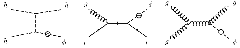
Figure 2: Representative Feynman diagrams giving contributing to $\phi$ freeze in production in the early universe. These processes determine $\rho_{\phi}$ which (in addition to $\rho_{\chi}$) determines the hidden sector’s temperature $T_{D}$. The effective vertex in the right diagram arises from integrating out the top quark for energies in between the weak scale and the QCD confinement scale (see Appendix B).

3.1 Boltzmann System

Our initial condition assumes a hot, radiation dominated universe in the broken electroweak phase. We further assume that $n_{\chi}=n_{\phi}=0$ after reheating so that sub-Hubble interactions with SM fields are solely responsible for populating the hidden sector. The Boltzmann equation for $\chi$ production is

$$\frac{dn_{\chi}}{dt}+3Hn_{\chi}=\langle\Gamma_{h\to\chi\chi}\rangle n_{h}-\langle\sigma v_{\chi\chi\to\rm SM}\rangle\!\left[n^{2}_{\chi}-n_{\chi}^{\rm eq}(T)^{2}\right]-\langle\sigma v_{\chi\chi\to\phi\phi}\rangle\!\left[n^{2}_{\chi}-n_{\chi}^{\rm eq}(T_{D})^{2}\right]\!,~{}~{}~{}$$ (6)

where $H\equiv 1.66\sqrt{g_{*}}T^{2}/m_{\rm\small Pl}$ is the Hubble rate during radiation domination, $m_{\rm Pl}=1.22\times 10^{-19}\,$ is the Planck mass, and $g_{*}$ is the number of relativistic degrees of freedom. Here an ^eq superscript denotes an equilibrium quantity, and we do not assume equilibrium between visible and hidden sectors $(T\neq T_{D})$; all relevant SM species are in equilibrium with each other, so we omit their superscript. As discussed above, existing bounds on the mixing angle require that the dark sector never thermalize with the SM in the early universe, so $n_{\chi}\ll n_{\chi}^{\rm eq}(T)$, but we allow for the possibility that $\chi\chi\longleftrightarrow\phi\phi$ annihilation (shown in the middle and right diagrams of Fig. 1) equilibrates the hidden sector so that $\chi$ eventually achieves a thermal distribution $n_{\chi}\to n_{\chi}^{\rm eq}(T_{D})$, where $T_{D}\ll T$. Thus, we can simplify the Boltzmann equation

$$\frac{dn_{\chi}}{dt}+3Hn_{\chi}=\langle\Gamma_{h\to\chi\chi}\rangle n_{h}+\langle\sigma v_{\chi\chi\to\rm SM}\rangle n_{\chi}^{\rm eq}(T)^{2}-\langle\sigma v_{\chi\chi\to\phi\phi}\rangle\!\left[n^{2}_{\chi}-n_{\chi}^{\rm eq}(T_{D})^{2}\right]\!,~{}~{}~{}$$ (7)

where the first two collision terms are independent of $n_{\chi}$ and serve merely as sources for $\chi$ production. In the limit where the hidden-sector annihilation rate is also sub-Hubble throughout the production process $\Gamma(\chi\chi\to\phi\phi)\ll H$, Eq. (7) recovers the usual freeze-in form in Eq. (2).

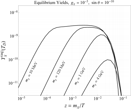
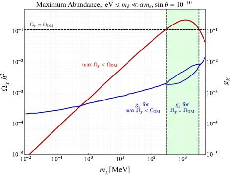
Figure 3: Left: Comoving equilibrium yields $Y^{\rm eq}_{\chi}=n_{\chi}^{\rm eq}(T_{D})/s(T)$ plotted against the dimensionless time variable $z=m_{\chi}/T$ for a various $m_{\chi}$. Note that the dark temperature is determined primarily by the $\phi$ energy density, which is independent of $m_{\chi}$, so each mass point has comparable $T_{D}$ during production; thus, sufficiently large masses are highly Boltzmann suppressed. Right: Maximum DM abundance for a range of $m_{\chi}$ with fixed $\sin\theta=10^{-10}$, which is still viable, but near the Red Giant exclusion bound (see left panel of Fig. 5). Below $m_{\chi}\lesssim 200$ MeV, the blue curve represents the coupling for which the maximum abundance (red curve) can be achieved; larger values merely annihilate away more of the DM as the number density tracks the equilibrium distributions (left) out to larger values of $z$ (see Fig 4, left). In the green band between the dashed vertical lines, ${\rm max}\,\Omega_{\chi}h^{2}>0.12$ so it is possible to achieve the full abundance for two choices of couplings, as shown for a representative mass point in Fig. 4.

3.2 Dark Temperature Evolution

In this scenario, the hidden sector temperature $T_{D}$ is defined in terms of the evolving dark sector energy density, which is also produced through SM interactions. The energy transfer Boltzmann equation for direct $\chi$ production is

$$\frac{d\rho_{\chi}}{dt}+3H(P_{\chi}+\rho_{\chi})={\cal P}_{h\to\chi\chi}n_{h}+{\cal P}_{hh\to\chi\chi}n_{h}^{2}+{\cal P}_{t\bar{t}\to\chi\chi}n_{t}^{2}+{\cal P}_{VV\to\chi\chi}n_{V}^{2},~{}~{}~{}~{}$$ (8)

and the contributions from mediator production (see Fig. 2) are

$$\frac{d\rho_{\phi}}{dt}+4H\rho_{\phi}=({\cal P}_{t\bar{t}\to g\phi}+{\cal P}_{t\bar{t}\to h\phi})\,n^{2}_{t}+{\cal P}_{tg\to t\phi}\,n_{t}n_{g}+{\cal P}_{th\to q\phi}\,n_{h}n_{t}+{\cal P}_{gg\to g\phi}\,n_{g}^{2},~{}~{}~{}~{}$$ (9)

and we define the thermally averaged quantity

$${\cal P}_{12\to 34}\equiv\frac{\int d^{3}p_{1}d^{3}p_{2}e^{-\frac{E_{1}\!+\!E_{2}}{T}}\Delta E\sigma_{12\to 34}v_{m\o}}{\int d^{3}p_{1}d^{3}p_{2}e^{-\frac{E_{1}\!+\!E_{2}}{T}}},~{}~{}~{}~{}~{}~{}~{}$$ (10)

where $\Delta E$ is the energy transferred to the hidden sector and $v_{m\o}$ is the Møller velocity (see Appendix A). Note that the definition of the energy transfer differs depending on whether we are considering $\chi$ pair production in Eq. (8) for which $\Delta E$ tracks both final state particles, or single $\phi$ production in Eq. (9) where it tracks only the energy transferred to $\phi$. The combined dark sector energy density $\rho_{D}=\rho_{\phi}+\rho_{\chi}$ defines a dark temperature

$$T_{D}\equiv\left(\frac{30\,\rho_{D}}{\pi^{2}\xi_{D}}\right)^{1/4},$$ (11)

where $\xi_{D}$ counts the relativistic degrees of freedom in the hidden sector. Note that the dark temperature initially satisfies $T_{D}=0$ and depends nontrivially on the visible temperature through Eqs. (8) and (9), which source its growth in Eq. (11). The dark temperature also determines the equilibrium $\chi$ number density in the hidden sector

$$n^{\rm eq}_{\chi}(T_{D})=\xi_{\chi}\int\!\frac{d^{3}p}{(2\pi)^{3}}e^{-E/T_{D}},$$ (12)

which enters into the RHS of Eq. (7). In our Boltzmann system we have omitted all processes involving lighter SM fermions, which only contribute negligibly to $\chi$ and $\phi$ production in the early universe; the dark sector is mainly populated while heavy electroweak states are in equilibrium with the SM thermal bath with corrections of order $\sim(m_{f}/m_{t})^{2}$ for all lighter SM fermions. For this reason, we can safely neglect longitudinal plasmon mixing effects which can resonantly enhance the $\phi$ production at lower temperatures for which $m_{\phi}$ is near the plasma frequency Hardy:2016kme ; this enhancement does not compensate for the parametric suppression in the coupling relative to continuum production off heavy electroweak states. However, such an effect may be important in model variations in which $\phi$ production arises mainly from its coupling to electrons (see Sec. 4 for a discussion). Although freeze-in is insensitive to the precise value of the reheat temperature, we assume it to be above $m_{t}$ for all SM electroweak states to be relativistic when dark sector production begins; if the reheat temperature is lower, DM production will proceed through lighter fermions and the resulting abundance will be significantly suppressed, but the qualitative features of our discussion are unaffected.

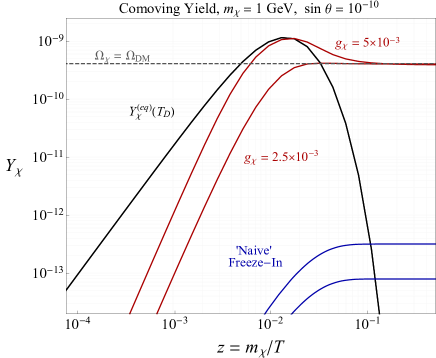
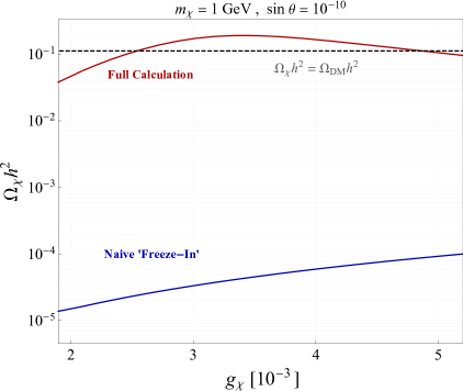
Figure 4: Left: Comoving yield $Y_{\chi}=n_{\chi}(T_{D})/s(T)$ for two representative $g_{\chi}$, which yield the observed DM abundance. Note that for both $g_{\chi}<2.5\times 10^{-3}$ and $g_{\chi}>5\times 10^{-3}$ the comoving yield is diminished. For reference, the blue curves at the bottom of the plot are the ‘naive’ freeze in result obtained by ignoring the $\chi,\phi$ dynamics in the hidden sector and merely integrating the SM source term in the Boltzmann equation from Eq.  (2). Right: Total $\chi$ abundance for fixed mass and coupling plotted alongside different choices of DM self coupling $g_{\chi}$. Note that the production history for the two points where the red curve intersects the dashed line are represented on the left panel.

3.3 Numerical Results

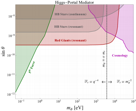
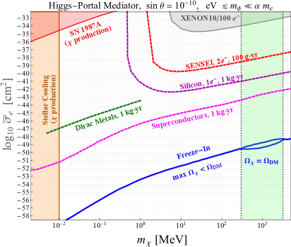
Figure 5: Left: Available parameter space for a light, Higgs-mixed scalar particle plotted alongside constraints from 5th forces Graham:2012su ; Kapner:2006si ; Geraci:2008hb ; Sushkov:2011zz ; Decca:2007jq ; Hoskins:1985tn , stellar cooling Hardy:2016kme , and cosmology Flacke:2016szy . The vertical line represents the approximate boundary where the $\chi e$ scattering rate undergoes a parametric shift for scattering off atomic electrons, which is taken to be the reference value for presenting different techniques in Battaglieri:2017aum . For other materials with different characteristic momenta, this shift takes place for different values of $m_{\phi}$. Right: Constraints and projections for the $\chi e$ cross section for sub-GeV DM. Some representative projections for the SENSEI $2e^{-}$, Silicon $1e^{-}$, and superconductor targets are taken from Battaglieri:2017aum , and the Dirac metals projection is from Hochberg:2017wce ; all projections assume $\Omega_{\chi}\Omega_{\rm DM}$. For points outside the green vertical band, the blue curve depicts $({\rm max}\,\Omega_{\chi}/\Omega_{\rm DM})\times\overline{\sigma}_{e}$ where sub-Hubble production as described in Sec. 3 generates the maximum fractional abundance (max $\Omega_{\chi}<\Omega_{\rm DM}$) for each $m_{\chi}$. Inside the vertical green band, the blue curves represent $\overline{\sigma}_{e}$ evaluated at $g_{\chi}$ for which the full DM abundance can be accommodated; note there are two such values as depicted in Fig. 4 and on the right panel of Fig. 3. Although the Higgs portal mixing $\sin\theta=10^{-10}$ may seem ad-hoc, this is chosen as a representative viable value near the stellar cooling exclusion region depicted on the left panel of this figure.

For the relevant parameter space considered in this paper $m_{\phi}\ll\alpha m_{e}$, the hidden sector temperature is primarily set by $\rho_{\phi}$ whose growth rate is proportional to $\sin^{2}\theta$ in Eq. (9), whereas the collision terms for $\rho_{\chi}$ in Eq. (8) all depend on $g_{\chi}^{2}\sin^{2}\theta$ and are further suppressed. Furthermore, $\rho_{\phi}$ continues to accumulate through $gg\to g\phi$ processes long after direct $\chi$ production processes (e.g. $tt\to\chi\chi$) have frozen out. Thus, the cosmological evolution of $T_{D}$ is insensitive to the DM mass, so sufficiently large values for which $m_{\chi}\ll T_{D}$ encounter hidden-sector Boltzmann suppression throughout their production, $\phi$-thermalization, and re-annihilation phases.

The left panel of 3 presents the equilibrium $\chi$ yield $Y_{\chi}^{\rm eq}\equiv n^{\rm eq}_{\chi}(T_{D})/s(T)$ normalized to the total entropy, where $n_{\chi}^{\rm eq}(T_{D})$ is computed using Eq. (12) and depends on the visible temperature implicitly through Eq. (11). Here we see that, as $m_{\chi}$ increases, the heights of these curves begin to fall, which ultimately limits the total abundance that can be generated for a given mass point; increasing $g_{\chi}$ increases the abundance in the freeze-in regime, but once the dark sector equilibrates with itself, the yield tracks these equilibrium distributions and eventually diminishes as more of the DM annihilates away into $\phi$ radiation. Thus, for each choice of mass there is a maximum abundance as represented by the red curve in Fig. 3 (right panel), which corresponds to the value of $g_{\chi}$ from the blue curve. Note that inside the green band, the blue curve splits into two segments corresponding to the distinct values that yield the observed DM abundance $\Omega_{\chi}h^{2}\simeq 0.12$, and not the maximum abundance (as it does outside this band).

This counterintuitive behavior can be understood from the plots in Fig. 4 which shows the production history for a representative mass point $m_{\chi}=$ and $\sin\theta=10^{-10}$ as the coupling $g_{\chi}$ is varied. On the left panel, the red curves are solutions to the Boltzmann equation in Eq. (7) for two choices of coupling that yield the observed DM abundance; the blue curves at the bottom of the plot also show the “naive” freeze-in result for the same choices of $g_{\chi}$; as in Eq. (2), the blue curves are computed by merely integrating the SM collision terms in Eq. (7) without including the additional $\chi\chi\longleftrightarrow\phi\phi$ dynamics. The right panel of Fig. 4 presents the DM abundance as a function of $g_{\chi}$ as computed with the full Boltzmann system (red curve) and with the naive freeze-in integration (blue curve).

On the right panel of Fig. 5 we present our main result: the predictive parameter space for $\chi$ production in the early universe plotted in terms of the fiducial $\chi e$ scattering cross section

$$\overline{\sigma}_{e}\equiv\frac{\mu^{2}_{\chi e}}{16\pi m_{\chi}^{2}m_{e}^{2}}\langle|{\cal A}(q_{0})|^{2}\rangle,$$ (13)

where ${\cal A}(q_{0})$ is the matrix element for a free-electron target evaluated at reference momentum $q_{0}=\alpha m_{e}$ following the convention in Battaglieri:2017aum , which also applies to the other projections shown. For the blue curve in this plot, this cross section is given by Eq. (5) in the $m_{\phi}\ll\alpha m_{e}$ limit and evaluated at $g_{\chi}$ values, which either yield the full DM abundance or the largest possible subdominant fraction where this is not possible as shown in Fig. 3 (right); in latter case the cross section is rescaled by the fractional abundance. The vertical green band in plot highlights the mass window for which the total abundance can be achieved and, as in Fig. 3 (right), the blue curve splits into two segments in the shaded green band to reflect the two values of $g_{\chi}$ that can accommodate the total abundance in; the top segment corresponds to $\chi$ that yield freeze-out in the hidden sector, whereas the bottom segment presents the freeze-in like value. Note that for most of the parameter points shown here max $\Omega_{\chi}\ll 10^{-2}\,\Omega_{\rm DM}$ (see Fig. 3, right), so DM self interaction bounds do not constrain the viable parameter space; for a discussion of this issue see Knapen:2017xzo . Relatedly, there is no perturbative unitary violation in $\chi\chi$ scattering for the $g_{\chi}$ along this curve since the values that yield the maximum possible abundance for viable choices of $\sin\theta$ are all well below unity (see Fig. 4, right). For completeness, we also show the viable parameter space for a Higgs portal mediator on the left panel of Fig. 5 to motivate our benchmarks.

4 Model Variations

Thus far, we have restricted our attention to the scenario in which both $\chi$ and $\phi$ are produced through $h$-$\phi$ mixing during the early universe. We have found that the bounds on $\sin\theta\lesssim 5\times 10^{-10}$ (see left panel of Fig 5), severely limit the total energy density transferred to the hidden sector, thereby making it impossible to achieve the total DM abundance for $m_{\chi}\lesssim$ few 100 MeV for all values of $g_{\chi}$. Here we consider some possible solutions to this problem that still feature sub-Hubble DM production and light scalar mediators.

4.1 Different SM Current

Since much of the discussion above depends on the Higgs-portal coupling relations, it may be possible to evade some of the above complications with a different pattern of couplings. For the scenario studied in this paper, the main impediment to generating the observed DM abundance over the $\lesssim m_{\phi}\lesssim\alpha m_{e}$ parameter space of interest is the limit $\sin\theta\lesssim 5\times 10^{-10}$, which is driven primarily by resonantly enhanced $\phi$ production through its coupling to electrons in Red Giants (RG) Hardy:2016kme – see Fig. 5 (left). For a minimal Higgs-mixing scenario, the same mixing angle $\theta$ rescales the $\phi$ coupling to electroweak states and thereby also suppresses the total energy energy/number density transferred to the hidden sector via electroweak production in the early universe. However, the early universe production is dominated by the heaviest SM states ($t$, $h$, $W/Z$) at $T\sim v$, so if the $\phi$ coupling to these particles can be enhanced relative to the electron coupling in a minimal Higgs-mixing scenario it is possible to increase the overall abundance at late times.

4.1.1 Two Higgs Doublets

One simple extension, which can accommodate such a variation involves mixing $\phi$ with the the neutral CP-even states of a two-Higgs doublet model (2HDM) to break the usual SM relations between quark and lepton couplings. For instance, in a Type II 2HDM, $\phi$ could mix with the predominantly up-type doublet, thereby increasing the relative ratio of $t/e$ couplings and enhancing dark sector particle production in electroweak processes. However, it is not clear whether a concrete realization of such a scenario can simultaneously accommodate the observed DM abundance while satisfying the existing limits on 2HDMs, which typically force the $\simeq 125$ GeV CP even scalar close to alignment limit, which approximately reproduces the usual SM coupling patters Khachatryan:2014jya ; ATLAS:2014kua , so a careful study is necessary to see if this is possible.

4.1.2 Vectorlike Fermions

Alternatively, the scalar mediator can couple to heavy vectorlike quarks, which are integrated out to induce effective interactions with SM particles (e.g. $\phi\,G_{\mu\nu}G^{\mu\nu}$, $\phi\,F_{\mu\nu}F^{\mu\nu}$, or $\phi\,\overline{q}q$ if vectorlike states mix with SM quarks). If the vectorlike quarks are sufficiently decoupled, all dark sector production proceeds through effective SM interactions and therefore this class of models makes a firm prediction for the DM-SM scattering rate. Furthermore, in this variation there is no tree-level electron coupling, so Red Giant bounds can be significantly weakened Hardy:2016kme and more DM can be produced via freeze-in, but this scenario is harder to test with new detection techniques, most of which probe DM-electron scattering in various materials.

If, instead, the mediator couples to heavy vectorlike leptons, the IR theory will contain the $\phi\,F_{\mu\nu}F^{\mu\nu}$ operator (and also $\phi\,\bar{\ell}\ell$ if the new heavier states mix with right handed leptons). However, this variation does not ameliorate the Red Giant bounds, which now constrain all early-universe production. Unlike in the Higgs-mixing scenario, where production off heavier electroweak states in Eqs. (8) and ( 9) is parametrically enhanced relative to the electron scattering cross section, here the production and detection depend on the same couplings, so dark sector production is greatly suppressed. Although the dominant $\phi$ production in this leptophilic scenario occur at lower temperatures $T\sim m_{\phi}$ where there is a resonant enhancement from $\phi$–longitudinal-plasmon mixing, this effect has been found to be modest (order-few) relative to non-resonant continuum production in astrophysical contexts Hardy:2016kme , so it is unlikely to compensate for the large reduction in the overall rate. Nonetheless, a full calculation of resonant $\phi$ production at these lower temperatures is worth further investigation.

4.2 Asymmetric Freeze-In

For the the scenario considered in earlier sections, the abundance is ultimately limited by the additional $\chi\chi\to\phi\phi$ annihilation phase that becomes efficient at depleting the $\chi$ population for sufficiently large $g_{\chi}$. However, if the DM carries a conserved global quantum number and has an asymmetric population at late times, then increasing $g_{\chi}$ will not lead to further depletion once all antiparticles are annihilated away. In order to maintain the qualitative features of the scenario considered here (light mediator and sub-Hubble production), the freeze-in interaction that produces the DM must also satisfy the Sakharov conditions Sakharov:1967dj . Although models of asymmetric freeze-in have been proposed in the literature Hall:2010jx , the asymmetry they produce is suppressed by subtle cancellations Hook:2011tk and it is not clear whether these limitations can be overcome, but this problem deserves further study (see Unwin:2014poa for a discussion).

4.3 Additional Production Source

One simple way to enhance DM production is to introduce a new source of $\chi$ or $\phi$ production beyond just the Higgs portal coupling to SM particles in Eq. (4). For instance $\phi$ could also mix with a new, heavy singlet scalar $S$ which thermalizes with the SM in the early universe. Since the $S$-$\phi$ mixing angle is a new free parameter, it is possible to increase the $\chi$ and $\phi$ abundances via $S$ initiated scattering and decay processes, which still realize freeze-in production if this mixing is suitably small. However, this modification is no longer predictive and manifestly depends on presently unknown UV physics, thereby detracting somewhat from the appeal of the freeze-in mechanism.

In addition to changing the SM-$\phi$ flavor structure, the SM extensions discussed in Sec. 4.1 can provide additional production sources if the new heavier particles are populated on shell after reheating. New interactions from these states can enhance $\phi$ and $\chi$ production in the early universe, but the magnitude of this enhancement now depends on the details of the extended sector(s), which adds UV sensitivity to the production mechanism.

5 Concluding Remarks

The recent burst of creativity in devising new techniques sub-GeV direct detection may soon make it possible to probe feebly coupled “freeze-in” dark matter coupled to a very light $\ll$ mediator. However, the only predictive, UV complete example in which this has been demonstrated (DM coupled to an ultra-light dark-photon) has subtly special properties that may not generalize to other mediators. To understand how robustly such scenarios can be probed, we have studied the freeze-in production of dark matter through a light scalar mediator with Higgs portal mixing.

In our analysis we find that the recently updated stellar cooling bounds on light scalars have severe, generic implications for any such freeze-in scenario. Most notably, for any sufficiently light ($\ll$) scalar mediator, compensating for the suppression from this bound requires a large, order-one coupling to dark matter, which quickly thermalizes the dark sector with itself. Even though all interactions between dark and visible sectors remain slower than Hubble expansion, the dark sector’s separate thermal bath enables efficient dark matter annihilation into mediators, thereby depleting its abundance once the mediator–dark-matter coupling increases beyond the threshold for hidden sector thermalization. Thus, for each choice of dark matter mass and Higgs mixing-angle, there is a maximum cosmological abundance that can be accommodated if the dark sector is only produced through its interactions with the Standard Model. We find that for Higgs portal mixing-angles near the limit imposed by astrophysical bounds, it is impossible to generate the observed dark matter abundance except for a narrow window in the $\sim$ 100 MeV – few GeV range. Furthermore, even inside this range, the cross sections for direct detection off electron targets are several orders of magnitude below future sensitivity projections for proposed experimental techniques.

We have also considered some possible model variations, which may alter these conclusions and allow for successful freeze-in with a light ($\ll$ keV) scalar mediator. In order to produce more DM during the early universe, while satisfying astrophysical bounds (which mostly constrain the mediator-electron coupling), it may be possible to generalize the minimal Higgs-portal scenario sector to mix the mediator with a larger electroweak sector (possibly a 2HDM) and thereby enhance the top-mediator coupling. This modification increases early universe freeze-in production while heavy electroweak states are still in equilibrium, but maintains an appreciable coupling to electrons for direct detection at late times. Similarly, it may be possible to enhance DM production by preferentially coupling the light mediator to a heavy vectorlike fourth generation of quarks, which are integrated out to generate higher dimension operators with SM quarks and gluons. Such a may alleviate astrophysical bounds on the mediator coupling and thereby enable viable freeze in production. Other possible variations include either additional (beyond Standard Model) sources of mediator or DM production and/or additional CP violation to realize a light-mediator variation on asymmetric freeze-in, but these possibilities are beyond the scope of the present work and deserve further study.

Acknowledgments: We thank Asher Berlin, Rouven Essig, Roni Harnik, Ciaran Hughes, Seyda Ipek, Yonatan Kahn, Simon Knapen, Robert Lasenby, Sam McDermott, Gopi Mohlabeng, Maxim Pospelov, and Brian Shuve for helpful conversations. Fermilab is operated by Fermi Research Alliance, LLC, under Contract No. DE- AC02-07CH11359 with the US Department of Energy.

Appendix A: Thermal Averaging

In this appendix we apply the methods used in Gondolo:1990dk to compute thermal averages for annihilation cross sections and energy transfer rates in the early universe.

Number Density Collision Terms

The full Boltzmann equation for DM depletion via $\chi(p_{1})\chi(p_{2})\to A(p_{3})B(p_{4})$ into SM final states $A$ and $B$ is

$$\frac{dn_{\chi}}{dt}+3Hn_{\chi}=C_{n},$$ (A.1)

$H\equiv\dot{a}/a=1.66\sqrt{g_{*}}T^{2}/m_{Pl}$ is the Hubble expansion rate during radiation domination and the collision term for the number density is

$$C_{n}=\!\int\!\prod_{i=1}^{4}\frac{d^{3}p_{i}}{2E_{i}(2\pi)^{3}}(2\pi)^{4}\delta^{4}\bigl{(}\textstyle{\sum}_{j}\,p_{j}\bigr{)}\langle\,|{\cal M}|^{2}\rangle\!\bigl{[}f^{\rm eq}_{A}(p_{3})f^{\rm eq}_{B}(p_{4})-f_{\chi}(p_{1})f_{\chi}(p_{2})\bigr{]},$$ (A.2)

where $\langle\,|{\cal M}|^{2}\rangle$ is the spin averaged squared matrix element and we have omitted bose(pauli) enhancement(blocking) factors. Using detailed balance $f^{\rm eq}_{\chi}(p_{1})f^{\rm eq}_{\chi}(p_{2})=f_{A}^{\rm eq}(p_{3})f^{\rm eq}_{B}(p_{4})$ and following the derivation in Gondolo:1990dk , the Botlzmann equation becomes

$$\frac{dn_{\chi}}{dt}+3Hn_{\chi}=-\langle\sigma v_{\chi\chi\to AB}\rangle\left[n_{\chi}^{2}-(n^{\rm eq}_{\chi})^{2}\right],$$ (A.3)

where the thermally averaged annihilation cross section is defined to be

$$\langle\sigma v_{\chi\chi\to{AB}}\rangle\equiv\frac{1}{8m_{\chi}^{4}TK_{2}\bigl{(}\frac{m_{\chi}}{T}\bigr{)}^{2}}\int_{4m_{\chi}^{2}}^{\infty}ds\,\sigma_{\chi\chi\to\phi\phi}\sqrt{s}(s-4m_{\chi}^{2})K_{1}\biggl{(}\frac{\sqrt{s}}{T}\biggr{)},~{}~{}~{}~{}$$ (A.4)

where $K_{1,2}$ are Bessel functions of the first and second kinds, respectively.

In the traditional “Freeze In” regime, the initial condition is $n_{\chi}(0)=0$ and the $\chi$ production rate in SM annihilation processes is slower than Hubble expansion, so the $n^{2}_{\chi}$ term can be neglected and the Boltzmann equation becomes integrable

$$\frac{dn_{\chi}}{dt}+3Hn_{\chi}=\langle\sigma v_{\chi\chi\to AB}\rangle(n^{\rm eq}_{\chi})^{2},$$ (A.5)

and we can define comoving yields $Y_{i}\equiv n_{i}/s$ and change the time variable to $z\equiv m_{\chi}/T$ to obtain

$$\frac{dY_{\chi}}{dz}=\frac{\langle\sigma v_{\chi\chi\to AB}\rangle s}{Hz}(Y^{\rm eq}_{\chi})^{2},$$ (A.6)

which can be integrated to obtain the asymptotic abundance at late times

$$\Omega_{\chi}=\frac{m_{\chi}s_{0}}{\rho_{\rm cr}}\,Y_{\chi}(\infty)=\frac{m_{\chi}s_{0}}{\rho_{\rm cr}}\int_{0}^{\infty}\frac{dz}{Hz}s\langle\sigma v_{\chi\chi\to AB}\rangle(Y^{\rm eq}_{\chi})^{2},$$ (A.7)

where $s_{0}\simeq 2969^{-3}$ is the present day CMB temperature, $\rho_{\rm cr}=8.1h^{2}\times 10^{-47}\,{}^{4}$ is the critical density.

Energy Density Collision Terms

Here we generalize the argument in Gondolo:1990dk to calculate the thermally averaged energy transferred to particle $1$ (which we will later identify with $\chi$ or $\phi$) in a $1+2\longleftrightarrow 3+4$ process governed by the Boltzmann equation

$$\frac{d\rho_{1}}{dt}+4H(P_{1}+\rho_{1})=C_{\rho},$$ (A.8)

Ignoring quantum statistical factors and assuming the other particles are in equilibrium with the radiation bath, the collision term is

$$C_{\rho}=\!\int\!\prod_{i=1}^{4}\frac{d^{3}p_{i}}{2E_{i}(2\pi)^{3}}(2\pi)^{4}\delta^{4}\bigl{(}\textstyle{\sum}_{j}\,p_{j}\bigr{)}\langle\,|{\cal M}|^{2}\rangle E_{1}\bigl{[}f_{3}^{\rm eq}(p_{3})f^{\rm eq}_{4}(p_{4})-f_{1}(p_{1})f_{2}^{\rm eq}(p_{2})\bigr{]},$$ (A.9)

where we make no assumption about particle $1$ being in thermal equilibrium with the others. Using detailed balance $f_{3}^{\rm eq}(p_{3})f_{4}^{\rm eq}(p_{4})=f_{1}^{\rm eq}(p_{1})f_{2}^{\rm eq}(p_{2})$ and the definition of the cross section

$$\sigma_{12\to 34}=\frac{1}{4F}\int\frac{d^{3}p_{3}}{2E_{3}(2\pi)^{3}}\frac{d^{3}p_{4}}{2E_{4}(2\pi)^{3}}(2\pi)^{4}\delta^{4}\bigl{(}\textstyle{\sum}_{j}\,p_{j}\bigr{)}\langle\,|{\cal M}|^{2}\rangle,\!$$ (A.10)

where $F=\sqrt{(p_{1}\cdot p_{2})^{2}-m_{1}^{2}m_{2}^{2}}$ is the usual flux factor, so we get

$$C_{\rho}=\!\int\!\frac{d^{3}p_{1}}{2E_{1}(2\pi)^{3}}\frac{d^{3}p_{2}}{2E_{2}(2\pi)^{3}}4F\sigma_{12\to 34}E_{1}f^{\rm eq}_{2}(p_{2})\bigl{[}f^{\rm eq}_{1}(p_{1})-f_{1}(p_{1})\bigr{]}.$$ (A.11)

Since the production/absorption rate is always slower than Hubble expansion for our purposes, the $f_{1}$ term can be neglected, so we get

$$C_{\rho}=\!\int\!\frac{d^{3}p_{1}}{2E_{1}(2\pi)^{3}}\frac{d^{3}p_{2}}{2E_{2}(2\pi)^{3}}4F\sigma_{12\to 34}\,E_{1}f^{\rm eq}_{1}(p_{1})f^{\rm eq}_{2}(p_{2})={\cal P}_{12\to 34}\,n^{\rm eq}_{2}n^{\rm eq}_{1},$$ (A.12)

where the thermally averaged power transfer rate is

$${\cal P}_{12\to 34}\equiv\frac{\int d^{3}p_{1}d^{3}p_{2}e^{-\frac{E_{1}\!+\!E_{2}}{T}}E_{1}\sigma_{12\to 34}v_{m\o}}{\int d^{3}p_{1}d^{3}p_{2}e^{-\frac{E_{1}\!+\!E_{2}}{T}}},~{}~{}~{}~{}~{}~{}~{}$$ (A.13)

and where the Møller velocity is $v_{m\o}\equiv F/E_{1}E_{2}$. the thermally averaged power is and denominator factor can be evaluated analytically

$$\!\!\int\!d^{3}p_{1}d^{3}p_{2}e^{-\frac{E_{1}\!+\!E_{2}}{T}}\!=(4\pi m_{1}m_{2}T)^{2}K_{2}\!\left(\frac{m_{1}}{T}\!\right)K_{2}\!\left(\frac{m_{2}}{T}\!\right).~{}~{}~{}~{}~{}~{}~{}$$ (A.14)

To evaluate the numerator of Eq. (A.13), we follow the procedure in Gondolo:1990dk we perform all trivial angular integrations and perform the coordinate transformation $(E_{1},E_{2}\cos\theta)\to(E_{+},E_{-},s)$ where $\theta$ is the CM angle between the incoming three-vectors, $E_{\pm}=E_{+}\pm E_{-}$, and $s=(p_{1}+p_{2})^{2}$ to get

$$\int d^{3}p_{1}d^{3}p_{2}e^{-\frac{E_{1}\!+\!E_{2}}{T}}E_{1}\sigma v_{m\o} = 2\pi^{2}\!\int_{s_{0}}^{\infty}ds\int^{\infty}_{\sqrt{s}}dE_{+}\int_{-\varepsilon}^{\varepsilon}dE_{-}\,e^{-E_{+}/T}\sigma_{12\to 34}E^{2}_{1}E_{2}v_{m\o}$$ (A.15)

$$= 2\pi^{2}T\!\int_{s_{0}}^{\infty}\!ds\,\sigma_{12\to 34}s\sqrt{1-\frac{s_{0}}{s}}K_{2}\!\left(\frac{\sqrt{s}}{T}\right),$$

where we have used $\varepsilon=\sqrt{1-s_{0}/s}\sqrt{E_{+}^{2}-s}$, so the power transfer becomes

$${\cal P}_{12\to 34}=\frac{1}{8m^{2}_{1}m^{2}_{2}TK_{2}\!\left(\frac{m_{1}}{T}\!\right)K_{2}\!\left(\frac{m_{2}}{T}\!\right)}\!\int_{s_{0}}^{\infty}\!\!ds\,\sigma_{12\to 34}\,sF\sqrt{1-\frac{s_{0}}{s}}K_{2}\!\left(\!\frac{\sqrt{s}}{T}\right),$$ (A.16)

which is valid even in the $m_{i}\to 0$ limit provided that the Bessel functions are properly expanded to cancel the mass dependence in the prefactor. Using detailed balance, we can relate the resulting collision term to the reverse process

$${\cal P}_{12\to 34}\,n_{1}^{\rm eq}n_{2}^{\rm eq}={\cal P}_{34\to 12}\,n_{3}^{\rm eq}n_{4}^{\rm eq},$$ (A.17)

which describes the SM+SM $\to$ SM $\phi$ processes in Eq. (9) where we identify $\phi$ with particle 1 of this argument.

For processes in which 2$\chi$ particles are produced via SM annihilation, a similar argument yields the expression

$${\cal P}_{\chi\chi\to AB}=\frac{1}{8m_{\chi}^{4}TK_{2}\bigl{(}\frac{m_{\chi}}{T}\bigr{)}^{2}}\int_{4m_{\chi}^{2}}^{\infty}ds\,\sigma_{\chi\chi\to AB}\,s(s-4m_{\chi}^{2})K_{2}\biggl{(}\frac{\sqrt{s}}{T}\biggr{)},~{}~{}~{}~{}$$ (A.18)

which tracks the energy transfer to both hidden sector particles produced in this process. whose form is appropriate for the collision terms in Eq. (8).

Appendix B: Cross Sections

DM Hidden Sector Annihilation $\chi\chi\to\phi\phi$

In the hidden sector, the $\chi\chi\to\phi\phi$ annihilation cross section is

$$\sigma_{\chi\chi\to\phi\phi}=\frac{g_{\chi}^{4}}{16\pi s^{2}(s-4m_{\chi}^{2})}\left[(s^{2}-16m_{\chi}^{2}s-32m_{\chi}^{4})\coth^{-1}\!\beta_{\chi}^{-1}-(s-8m_{\chi}^{2})\sqrt{s(s-4m_{\chi}^{2})}\,\right],~{}~{}~{}~{}~{}~{}$$ (B.1)

where we have taken the limit $m_{\chi}\gg m_{\phi}$, which is appropriate for the full range of parameters we consider in this work. The thermal average has the familiar form, but evaluated at the hidden sector temeprature

$$\langle\sigma v_{\chi\chi\to\phi\phi}\rangle=\frac{1}{8m_{\chi}^{4}TK_{2}\bigl{(}\frac{m_{\chi}}{T_{D}}\bigr{)}^{2}}\int_{4m_{\chi}^{2}}^{\infty}ds\,\sigma_{\chi\chi\to\phi\phi}\sqrt{s}(s-4m_{\chi}^{2})K_{1}\biggl{(}\frac{\sqrt{s}}{T_{D}}\biggr{)},~{}~{}~{}~{}$$ (B.2)

which depends on the visible temperature through Eqs. (8) and (11).

Direct DM Production $h\to\chi\chi$

$$\Gamma_{h\to\chi\chi}=\frac{g_{\chi}^{2}\sin^{2}\!\theta\,m_{h}}{8\pi}\left(1-\frac{4m_{\chi}^{2}}{m_{h}^{2}}\right)^{3/2},~{}~{}$$ (B.3)

Direct DM Production $\chi\chi\to ff$

The cross section for $\chi$ annihilation into SM fermions $f$ is given by

$$\sigma_{\chi\chi\to ff}=\frac{g_{\chi}^{2}\sin^{2}\!\theta\,m_{f}^{2}}{16\pi v^{2}s}\beta_{f}^{3}\,\beta_{\chi}~{},~{}~{}$$ (B.4)

where we have defined $\beta_{i}\equiv\sqrt{1-4m_{i}^{2}/s}$

Direct DM Production: Higgs Annihilation $\chi\chi\to hh$

$$\sigma_{\chi\chi\to hh}=\frac{9g_{\chi}^{2}\sin^{2}\!\theta\,m_{h}^{4}}{32\pi v^{2}s^{2}}\left(1-\frac{4m_{\chi}^{2}}{s}\right)\sqrt{\frac{s-4m_{h}^{2}}{s-4m_{\chi}^{2}}}~{},~{}~{}$$ (B.5)

Direct DM Production: Vector Annihilation $\chi\chi\to VV$

$$\sigma_{\chi\chi\to VV}=\frac{\,g_{\chi}^{2}\sin^{2}\!\theta\,m_{h}^{4}(s-4m_{\chi}^{2})(12m_{V}^{4}-4m_{V}^{2}s+s^{2})}{72\pi v^{2}s^{3}}\sqrt{\frac{s-4m_{V}^{2}}{s-4m_{\chi}^{2}}}~{},~{}~{}$$ (B.6)

Mediatior Production: Electroweak Scalar Annihilation $ff\to h\phi$

For each fermion $f$ there are three contributions to the $f(p_{1})\bar{f}(p_{2})\to\phi(p_{3})h(p_{4})$ process

$${\cal M}(f\bar{f}\to\phi h)=-\sin\theta\,\overline{u}(p_{1})\left(\frac{m_{f}^{2}}{v^{2}}\frac{(\displaystyle{\not}{p_{1}}-\displaystyle{\not}{p_{3}}+m_{f})}{t-m_{f}^{2}}+\frac{m_{f}^{2}}{v^{2}}\frac{(\displaystyle{\not}{p_{1}}-\displaystyle{\not}{p_{4}}+m_{f})}{u-m_{f}^{2}}+\frac{3m_{h}^{2}m_{f}}{v^{2}}\frac{1}{s-m_{h}^{2}}\right)v(p_{2}),~{}~{}~{}~{}~{}~{}~{}$$ (B.7)

where we have also included the $s$-channel diagram involving the trilinear scalar interaction. We calculate the total cross section using FeynCalc Shtabovenko:2016olh

Mediatior Production: Electroweak Scalar Compton $fh\to f\phi$

As above, the higgs-fermion scattering process $h(p_{1})f(p_{2})\to\phi(p_{3})f(p_{4})$ is represented by three Feynman diagrams with amplitude

$${\cal M}(hf\to\phi f)=-\sin\theta\,\overline{u}(p_{2})\left(\frac{m_{f}^{2}}{v^{2}}\frac{(\displaystyle{\not}{p_{1}}+\displaystyle{\not}{p_{2}}+m_{f})}{s-m_{f}^{2}}+\frac{m_{f}^{2}}{v^{2}}\frac{(\displaystyle{\not}{p_{2}}-\displaystyle{\not}{p_{3}}+m_{f})}{u-m_{f}^{2}}+\frac{3m_{h}^{2}m_{f}}{v^{2}}\frac{1}{t-m_{h}^{2}}\right)u(p_{4}).~{}~{}~{}~{}~{}~{}~{}$$ (B.8)

We calculate the total cross section using FeynCalc Shtabovenko:2016olh where we sum over colors and average over spins.

Mediatior Production: Higgs Semi Annihilation $hh\to h\phi$

The cross section for $\phi$ production via Higgs semi annihilation is

$$\sigma_{hh\to h\phi}=\frac{9m_{h}^{4}\sin^{2}\!\theta}{16\pi v^{4}(s-4m_{h}^{2})(s-m_{h}^{2})}\left[(s+2m_{h}^{2})(s+8m_{h}^{2})\beta_{h}+24m_{h}^{2}(s-m_{h}^{2})\tanh^{-1}\beta_{h}\,\right],~{}~{}~{}~{}~{}$$ (B.9)

where $\beta_{h}\equiv\sqrt{1-4m_{h}^{2}/s}$ and we have taken the $m_{\phi}\to 0$ limit, appropriate for the early universe while the Higgs is still part of the thermal bath.

Mediatior Production: QCD Annihilation $ff\to g\phi$

Our main focus will be annihilation off SM top quarks with cross section

$$\sigma_{f\bar{f}\to g\phi}=\frac{4\alpha_{s}\sin^{2}\!\theta\,m_{f}^{2}}{s(s-4m_{f}^{2})v^{2}}\left[(s+4m_{f}^{2})\tanh^{-1}\beta_{f}-(s-2m_{f}^{2})\beta_{f}\right],~{}~{}~{}~{}$$ (B.10)

where we have summed (not averaged) over all colors to keep track of all degrees of freedom that enter into the collision term of the Boltzmann equations.

Mediatior Production: QCD Compton $fg\to f\phi$

For the QCD compton process, we have

$$\sigma_{fg\to f\phi}=\frac{\alpha_{s}\sin^{2}\!\theta\,m_{f}^{2}}{2s^{2}(s-m_{f}^{2})^{3}v^{2}}\left[(s-m_{f}^{2})(3s+m_{f}^{2})(m_{f}^{4}-8m_{f}^{2}s-s^{2})+2s^{2}(s+3m_{f}^{2})^{2}\log\frac{s}{m_{f}^{2}}\right],~{}~{}~{}~{}~{}$$ (B.11)

where we have summed (not averaged) over colors to account for all relevant degrees of freedom in the thermal bath.

Mediatior Production: Glue Scatter $gg\to g\phi$

For $m_{t}\gg T\gg m_{\phi}$, we can integrate out the top quark and evaluate the scattering process $gg\to g\phi$ which remains effective until confinement around $T\sim\Lambda_{\rm QCD}\approx 200\,$. Neglecting $m_{\phi}$, the differential rate for this process is

$$\frac{d\sigma_{gg\to g\phi}}{dt}=-\frac{\pi^{2}\alpha_{s}^{3}(s^{2}+st+t^{2})^{2}}{12v^{2}s^{3}t(s+t)},$$ (B.12)

where again we have summed (but not averaged) over all colors. Note that the RHS is always positive in the physical phase space where $t<0$ and that there is a $t$-channel, forward scattering singularity as $t\to 0$, which is regulated by the QCD Debye mass $m^{2}_{g}(T)=8\pi\alpha_{s}T^{2}$ at finite temperature.

References

- (1) G. Bertone and D. Hooper, A History of Dark Matter, Submitted to: Rev. Mod. Phys. (2016) , [1605.04909].
- (2) L. Roszkowski, E. M. Sessolo and S. Trojanowski, WIMP dark matter candidates and searches - current issues and future prospects, 1707.06277.
- (3) J. Alexander et al., Dark Sectors 2016 Workshop: Community Report, 2016. 1608.08632.
- (4) M. Battaglieri et al., US Cosmic Visions: New Ideas in Dark Matter 2017: Community Report, 1707.04591.
- (5) R. Essig, J. Mardon and T. Volansky, Direct Detection of Sub-GeV Dark Matter, Phys. Rev. D85 (2012) 076007, [1108.5383].
- (6) R. Essig, A. Manalaysay, J. Mardon, P. Sorensen and T. Volansky, First Direct Detection Limits on sub-GeV Dark Matter from XENON10, Phys. Rev. Lett. 109 (2012) 021301, [1206.2644].
- (7) R. Essig, T. Volansky and T.-T. Yu, New Constraints and Prospects for sub-GeV Dark Matter Scattering off Electrons in Xenon, Phys. Rev. D96 (2017) 043017, [1703.00910].
- (8) Y. Hochberg, Y. Zhao and K. M. Zurek, Superconducting Detectors for Superlight Dark Matter, Phys. Rev. Lett. 116 (2016) 011301, [1504.07237].
- (9) Y. Hochberg, T. Lin and K. M. Zurek, Detecting Ultralight Bosonic Dark Matter via Absorption in Superconductors, Phys. Rev. D94 (2016) 015019, [1604.06800].
- (10) P. W. Graham, D. E. Kaplan, S. Rajendran and M. T. Walters, Semiconductor Probes of Light Dark Matter, Phys. Dark Univ. 1 (2012) 32–49, [1203.2531].
- (11) J. Tiffenberg, M. Sofo-Haro, A. Drlica-Wagner, R. Essig, Y. Guardincerri, S. Holland et al., Single-electron and single-photon sensitivity with a silicon Skipper CCD, Phys. Rev. Lett. 119 (2017) 131802, [1706.00028].
- (12) R. Essig, M. Fernandez-Serra, J. Mardon, A. Soto, T. Volansky and T.-T. Yu, Direct Detection of sub-GeV Dark Matter with Semiconductor Targets, JHEP 05 (2016) 046, [1509.01598].
- (13) H. J. Maris, G. M. Seidel and D. Stein, Dark Matter Detection Using Helium Evaporation and Field Ionization, Phys. Rev. Lett. 119 (2017) 181303, [1706.00117].
- (14) Y. Hochberg, M. Pyle, Y. Zhao and K. M. Zurek, Detecting Superlight Dark Matter with Fermi-Degenerate Materials, JHEP 08 (2016) 057, [1512.04533].
- (15) Y. Hochberg, Y. Kahn, M. Lisanti, K. M. Zurek, A. Grushin, R. Ilan et al., Detection of sub-MeV Dark Matter with Three-Dimensional Dirac Materials, 1708.08929.
- (16) Y. Hochberg, Y. Kahn, M. Lisanti, C. G. Tully and K. M. Zurek, Directional detection of dark matter with two-dimensional targets, Phys. Lett. B772 (2017) 239–246, [1606.08849].
- (17) P. C. Bunting, G. Gratta, T. Melia and S. Rajendran, Magnetic Bubble Chambers and Sub-GeV Dark Matter Direct Detection, Phys. Rev. D95 (2017) 095001, [1701.06566].
- (18) R. Budnik, O. Chesnovsky, O. Slone and T. Volansky, Direct Detection of Light Dark Matter and Solar Neutrinos via Color Center Production in Crystals, 1705.03016.
- (19) R. Essig, J. Mardon, O. Slone and T. Volansky, Detection of sub-GeV Dark Matter and Solar Neutrinos via Chemical-Bond Breaking, Phys. Rev. D95 (2017) 056011, [1608.02940].
- (20) M. Pospelov and J. Pradler, Big Bang Nucleosynthesis as a Probe of New Physics, Ann. Rev. Nucl. Part. Sci. 60 (2010) 539–568, [1011.1054].
- (21) A. Berlin and N. Blinov, Thermal Dark Matter Below an MeV, 1706.07046.
- (22) J. McDonald, Thermally generated gauge singlet scalars as selfinteracting dark matter, Phys. Rev. Lett. 88 (2002) 091304, [hep-ph/0106249].
- (23) L. J. Hall, K. Jedamzik, J. March-Russell and S. M. West, Freeze-In Production of FIMP Dark Matter, JHEP 03 (2010) 080, [0911.1120].
- (24) X. Chu, T. Hambye and M. H. G. Tytgat, The Four Basic Ways of Creating Dark Matter Through a Portal, JCAP 1205 (2012) 034, [1112.0493].
- (25) J. H. Chang, R. Essig and S. D. McDermott, Revisiting Supernova 1987A Constraints on Dark Photons, JHEP 01 (2017) 107, [1611.03864].
- (26) E. Hardy and R. Lasenby, Stellar cooling bounds on new light particles: plasma mixing effects, JHEP 02 (2017) 033, [1611.05852].
- (27) S. Knapen, T. Lin and K. M. Zurek, Light Dark Matter: Models and Constraints, 1709.07882.
- (28) F. Kahlhoefer, S. Kulkarni and S. Wild, Exploring light mediators with low-threshold direct detection experiments, JCAP 1711 (2017) 016, [1707.08571].
- (29) C. Kouvaris, I. M. Shoemaker and K. Tuominen, Self-Interacting Dark Matter through the Higgs Portal, Phys. Rev. D91 (2015) 043519, [1411.3730].
- (30) G. Krnjaic, Probing Light Thermal Dark-Matter With a Higgs Portal Mediator, Phys. Rev. D94 (2016) 073009, [1512.04119].
- (31) M. Kaplinghat, S. Tulin and H.-B. Yu, Dark Matter Halos as Particle Colliders: Unified Solution to Small-Scale Structure Puzzles from Dwarfs to Clusters, Phys. Rev. Lett. 116 (2016) 041302, [1508.03339].
- (32) P. Adshead, Y. Cui and J. Shelton, Chilly Dark Sectors and Asymmetric Reheating, JHEP 06 (2016) 016, [1604.02458].
- (33) A. Berlin, D. Hooper and G. Krnjaic, PeV-Scale Dark Matter as a Thermal Relic of a Decoupled Sector, Phys. Lett. B760 (2016) 106–111, [1602.08490].
- (34) A. Berlin, D. Hooper and G. Krnjaic, Thermal Dark Matter From A Highly Decoupled Sector, Phys. Rev. D94 (2016) 095019, [1609.02555].
- (35) D. J. Kapner, T. S. Cook, E. G. Adelberger, J. H. Gundlach, B. R. Heckel, C. D. Hoyle et al., Tests of the gravitational inverse-square law below the dark-energy length scale, Phys. Rev. Lett. 98 (2007) 021101, [hep-ph/0611184].
- (36) A. A. Geraci, S. J. Smullin, D. M. Weld, J. Chiaverini and A. Kapitulnik, Improved constraints on non-Newtonian forces at 10 microns, Phys. Rev. D78 (2008) 022002, [0802.2350].
- (37) A. O. Sushkov, W. J. Kim, D. A. R. Dalvit and S. K. Lamoreaux, New Experimental Limits on Non-Newtonian Forces in the Micrometer Range, Phys. Rev. Lett. 107 (2011) 171101, [1108.2547].
- (38) R. S. Decca, D. Lopez, E. Fischbach, G. L. Klimchitskaya, D. E. Krause and V. M. Mostepanenko, Novel constraints on light elementary particles and extra-dimensional physics from the Casimir effect, Eur. Phys. J. C51 (2007) 963–975, [0706.3283].
- (39) J. K. Hoskins, R. D. Newman, R. Spero and J. Schultz, Experimental tests of the gravitational inverse square law for mass separations from 2-cm to 105-cm, Phys. Rev. D32 (1985) 3084–3095.
- (40) T. Flacke, C. Frugiuele, E. Fuchs, R. S. Gupta and G. Perez, Phenomenology of relaxion-Higgs mixing, JHEP 06 (2017) 050, [1610.02025].
- (41) CMS collaboration, V. Khachatryan et al., Searches for heavy Higgs bosons in two-Higgs-doublet models and for decay using multilepton and diphoton final states in collisions at 8 TeV, Phys. Rev. D90 (2014) 112013, [1410.2751].
- (42) ATLAS collaboration, T. A. collaboration, Constraints on New Phenomena via Higgs Coupling Measurements with the ATLAS Detector, .
- (43) A. Fradette and M. Pospelov, BBN for the LHC: constraints on lifetimes of the Higgs portal scalars, 1706.01920.
- (44) A. D. Sakharov, Violation of CP Invariance, c Asymmetry, and Baryon Asymmetry of the Universe, Pisma Zh. Eksp. Teor. Fiz. 5 (1967) 32–35.
- (45) L. J. Hall, J. March-Russell and S. M. West, A Unified Theory of Matter Genesis: Asymmetric Freeze-In, 1010.0245.
- (46) A. Hook, Unitarity constraints on asymmetric freeze-in, Phys. Rev. D84 (2011) 055003, [1105.3728].
- (47) J. Unwin, Towards cogenesis via Asymmetric Freeze-In: The who came-in from the cold, JHEP 10 (2014) 190, [1406.3027].
- (48) P. Gondolo and G. Gelmini, Cosmic abundances of stable particles: Improved analysis, Nucl. Phys. B360 (1991) 145–179.
- (49) V. Shtabovenko, FeynCalc 9, J. Phys. Conf. Ser. 762 (2016) 012064, [1604.06709].