The seven sisters DANCe III.

Abstract

Context. Membership analyses of the DANCe and Tycho+DANCe data sets provide the largest and least contaminated sample of Pleiades candidate members to date.

Aims. We aim at reassessing the different proposals for the number surface density of the Pleiades in the light of the new and most complete list of candidate members, and inferring the parameters of the most adequate model.

Methods. We compute the Bayesian evidence and Bayes Factors for variations of the classical radial models. These include elliptical symmetry, and luminosity segregation. As a by-product of the model comparison, we obtain posterior distributions for each set of model parameters.

Results. We find that the model comparison results depend on the spatial extent of the region used for the analysis. For a circle of 11.5 parsecs around the cluster centre (the most homogeneous and complete region), we find no compelling reason to abandon King’s model, although the Generalised King model introduced here has slightly better fitting properties. Furthermore, we find strong evidence against radially symmetric models when compared to the elliptic extensions. Finally, we find that including mass segregation in the form of luminosity segregation in the J band is strongly supported in all our models.

Conclusions. We have put the question of the projected spatial distribution of the Pleiades cluster on a solid probabilistic framework, and inferred its properties using the most exhaustive and least contaminated list of Pleiades candidate members available to date. Our results suggest however that this sample may still lack about 20% of the expected number of cluster members. Therefore, this study should be revised when the completeness and homogeneity of the data can be extended beyond the 11.5 parsecs limit. Such a study will allow for more precise determination of the Pleiades spatial distribution, its tidal radius, ellipticity, number of objects and total mass.

1 Introduction

The projected spatial distribution (PSD), also known as number surface density, of a stellar cluster is the two dimensional (2D) projection, in the plane of the sky, of its three dimensional (3D) space distribution. Because celestial coordinates are far more easily measured than parallaxes (at least before Gaia), only a small fraction of the objects with stellar positions have distance estimates. Furthermore, the relative uncertainties in the celestial coordinates yield far more precise measurements (by a factor of $10^{4}$) of distances perpendicular to the line of sight than those achieved by parallaxes along this line so far (except perhaps for very close objects). This explains why most of the previous works devoted to studying the spatial distribution of stars in clusters have been done using the PSD.

In the case of the Pleiades, cross-matching the Hipparcos catalogue (Perryman et al. 1997) with the 2109 candidate members of Bouy et al. (2015), shows that only 70 of them have parallax measurements. This figure has roughly doubled with the first Gaia data release DR1 (Gaia Collaboration et al. 2016), and is expected to improve based on the longer time baselines and hence more accurate measurements of subsequent Gaia releases. In preparation for the analysis of these upcoming data sets and to narrow down the set of models that will be tested in the context of 3D studies, we have initiated a re-examination of the current analytical alternatives to describe the PSD of the Pleiades cluster.

The Pleiades PSD has been thoroughly studied in the past. Pinfield et al. (1998) fitted King’s (King 1962, hereafter King’s) empirical profiles to the positions of $1194$ candidate members from the literature, which were contained in a $3^{\circ}$ radius area. For their fitted King profiles, they used different mass ranges, with bins centred at $5.2,1.65,0.83$ and $0.3\,\mathrm{M_{\odot}}$. Using tidal forces, they iteratively constrained the tidal radius to a value of $13.1$ pc ($\sim 5.6^{\circ}$). They infer a core radii in the 0.9-2.91 pc range in the different mass bins, and a total mass of $735\,\mathrm{M_{\odot}}$. They interpreted the gradual increase in the core radii for decreasing mass ranges as evidence of mass segregation.

The same year, Raboud & Mermilliod (1998) also fitted a King’s profile to a list of 270 candidate members with masses in the range $0.74-7.04\,\mathrm{M_{\odot}}$, which were contained within a $5^{\circ}$ radius area. They found a core radius of $1.5$ pc and a tidal radius of $17.5$ pc ($7.5$ degrees). Using different approaches, they derived a total mass within the range of $500-8000\,\mathrm{M_{\odot}}$. They also measured an ellipticity of $\epsilon=0.17$. However, they did not make any explicit mention of the position angle of the axis of the ellipse, and simply state that it is roughly parallel to the galactic equator.

Later, Adams et al. (2001) also fitted a King’s profile to objects with membership probabilities $p>0.3$ within a radius of $10^{\circ}$. They found a core radius of $2.35-3.0$ pc and a tidal radius of $13.6-16$ pc ($5.8-6.8^{\circ}$). They estimate a total mass of $\sim 800\,\mathrm{M_{\odot}}$, and their measured ellipticities are in the range $0.1-0.35$.

Converse & Stahler (2008) fitted a King’s profile to a sample of 1245 candidate members from the Stauffer et al. (2007) compilation. These objects have masses greater than $0.08\,\mathrm{M_{\odot}}$ and are contained within a $5^{\circ}$ radius. They obtained a tidal radius of $18$ pc ($7.7^{\circ}$) and a core radius of $1.3$ pc. They found unambiguous evidence of mass segregation using a method they devised inspired by econometrics. Later, Converse & Stahler (2010) refined their previous study (Converse & Stahler 2008) and obtained a core radius of $2.0\pm 0.1$ pc, a tidal radius of $19.5\pm 1.0$ pc ($\sim 8.3$ degrees), a total number of systems of 1256$\pm$35, and a total mass of $870\pm 35\,\mathrm{M_{\odot}}$.

The previous summary of results shows at least two interesting points. In the first place, the King’s profile has been the preferred choice for the Pleiades cluster, although it was created to fit the PSD of globular clusters. Since globular clusters are farther away than open clusters and in a low-density environment, the end of their PSD is usually well within the survey area, which is not the case for the Pleiades. The second point concerns the increasing trend of the tidal radius with the size of the survey and the publication date (Table 1); as the surveys increase in area, the derived tidal radii increase as well. This may indicate that truncation has not been accounted for (see Appendix A and Fig. 6 particularly). The exception to this trend is the work of Adams et al. (2001), in which the tidal radius is well within the survey radius. Since these authors used low-membership-probability ($\geq 0.3$) objects, their results may be affected by a significant contamination rate, which these authors acknowledge for their $>5^{\circ}$ sample.

The two points mentioned above are tightly related. With the exception of the work of Adams et al. (2001), the coverages of the rest of the surveys have not reached their estimated tidal radius. This indicates that the previously used samples of members were spatially truncated. They only contain objects from the inner parts of the cluster. Thus, estimates of the tidal radius may have been biased, and were, in any case, highly correlated with the contamination rate.

Table 1: Survey, and derived core and tidal radius for recent studies in the literature.

	Core	Tidal	Survey
	radius	radius	radius
	(pc)	(pc/∘)	(∘)
Pinfield et al. (1998)	0.9-2.91	13.1/5.6	3
Raboud & Mermilliod (1998)	1.5	17.5/7.5	5
Adams et al. (2001)	2.35-3.0	16/6.8	10
Converse & Stahler (2008)	1.3	18/7.7	5
Converse & Stahler (2010)	2.0	19.5/8.3	5

With Gaia data coming up soon, we will have very accurate measurements of the spatial distribution of all the brightest ($G\leq 20$ mag) members of nearby clusters. Therefore, it is important to define sufficiently complex models to describe these measurements. The early and simple formulations of the PSD (e.g. King) were perfect when a dozen or a few tens of dozens of members were known. But the accuracy and completeness of future surveys will allow us to look in finer detail.

The study of the spatial distribution also has implications that go beyond its intrinsic interest. One of them is the existence of mass segregation as a result of star formation and dynamical interactions in the cluster. This effect has been predicted by numerical simulations of the internal cluster dynamics; see, for example, Terlevich (1987); Kroupa et al. (2001); Moraux et al. (2004); Converse & Stahler (2010). Confirming and quantifying its dependance on various parameters (e.g. initial mass function, core mass function, total mass of the cluster, presence or absence or massive stars, T- or OB- association) shall provide important input to the models and simulations of star formation and dynamical evolution.

In the specific case of the Pleiades, mass segregation has been reported in the works of Raboud & Mermilliod (1998); Pinfield et al. (1998); Kroupa et al. (2001); Adams et al. (2001); Moraux et al. (2004); Converse & Stahler (2008, 2010). Yet, Loktin (2006), using radial and tangential velocity dispersions, found no hint of mass segregation in a sample of 340 stars contained in the central $2.3^{\circ}$. However, his results may arise from the low number and extent of his sample. All the mentioned works performed their analyses by binning the stellar samples in mass or distance ranges. It is well known however that fitting a function to a binned data set can introduce biases (Bevington & Robinson 2003; Nousek & Shue 1989), and that modifying the bin width could improve the fitting to a preferred model (Towers 2012). Thus, the use of bins in previous works and the contradictory mass-segregation results found by Loktin (2006) may suggest that the hypothesis of mass segregation in the Pleiades requires a more solid reexamination.

In this work we aim at addressing this hypothesis on the basis of the largest and least contaminated sample of Pleiades candidate members found to date: the combined list of candidate members from Bouy et al. (2015) and Olivares et al. (2017). We avoid the binning biases by using Bayesian inference methods applied to continuous and thus non-binned distributions. In addition, these Bayesian methods allow a quantitative comparison of the competing models, including those with and without mass segregation. This will allow us to establish on firm grounds the analytical expression of the Pleiades PSD, and its potential dependence on stellar mass.

In Section 2 we briefly describe the data set that forms the basis of our analysis. In Section 3 we present the set of radially symmetric analytical models we used, as well as their extension to biaxially symmetric (elliptical) profiles. We also include a luminosity dependence of the core radius (as a proxy to the investigation of mass segregation). In Section 4 we describe the foundations of model selection in the Bayesian framework. We then discuss and compare the results that we obtain for the posterior distributions of the various models in Section 5, where we also briefly describe our estimates on the total mass and number of members in the cluster. Finally, in Section 6 we summarise the conclusions drawn from the study.

2 The data sample

The data set used to compare the models in Section 3 corresponds to the high-membership-probability candidate members of Olivares et al. (2017), in the middle and faint luminosity end, with the addition of the Tycho-2 Pleiades high-luminosity candidate members from Bouy et al. (2015). This joint data set comprises the equatorial coordinates R.A. and Dec. (in the following $\alpha$ and $\delta$), proper motions, photometry, and membership probabilities of 2060 sources. In this analysis we work only with the positions, membership probabilities, and J photometric band. The latter is the reddest most available band for this list of members, and is used as a proxy for the mass and to explore evidence of mass segregation.

2.1 Completeness of the sample

To properly establish the probabilistic framework, it is necessary to take into account the observational constraints of the data. The Pleiades DANCe catalogue is constrained by its sky coverage and the different degrees of completeness (see Bouy et al. 2013, 2015, for details). Although the data set extends up to a radius of $6.5^{\circ}$, Bouy et al. (2015) conservatively assume that the census is homogeneous in coverage and limiting magnitude only in the central $3^{\circ}$ radius area.

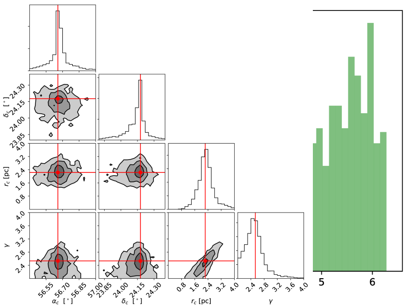
Figure 8: Projections of the posterior distribution for the radially symmetric EFF model.

Here, we estimate the completeness of the whole of the joint Tycho+DANCe survey in terms of the J band luminosity and spatial coverage, which also applies to our list of candidate members. In Fig. 1 we show the distributions of the number of sources in the combined DANCe+Tycho catalogue as a function of the radial position for different limiting magnitudes and bins in the J band. The radial position is computed assuming a distance of 134.4 pc to the Pleiades cluster (Galli et al. 2017) and a centre at $\alpha,\delta=[56.65,24.13]$. As can be seen from the top panel of this Figure, the DANCe+Tycho catalogue is spatially complete until a radial distance of 11.5 pc ($\sim 5^{\circ}$). The latter corresponds roughly to the sky coverage of the UKIDSS survey (Lawrence et al. 2007). Above this limit, the density of sources drops with two different slopes. The first one is created by the sawtooth pattern at the edge of the DANCe survey, while the last one corresponds to the more extended selection box used for the Tycho survey. To evaluate the photometric completeness, we assume that the distribution of sources in the sky region of the Pleiades is uniform (this simplistic assumption is sufficient for our current purpose). We compare the radial density of sources of different J magnitude bins with that of a synthetic sample uniformly distributed in space and truncated at the completeness radius of 11.5 pc. The radial distribution of this synthetic sample and those of the three magnitude bins are shown in the bottom panel of Fig. 1. As can be seen from the latter, the joint Tycho+DANCe survey is expected to be complete until magnitude $\sim 19$ in the J band. Above this limit, the distribution of sources departs significantly from the expected one. Hence, we restrict our list of candidate members to those with: i) J band observed and less than 19 mag., and ii) radial distances less than 11.5 pc. This results in 1954 candidate members, which represents more than 50% more candidate members than those of Converse & Stahler (2010), who did the latest analysis of the Pleiades PSD. Accounting for completeness and the previous truncation in the data set is essential to avoid possible bias in the inferred parameters (see Appendix A). Nevertheless, we remind the reader that the inhomogeneities (e.g. spatial resolutions, gaps in luminosity) of the DANCe+Tycho data set are so complex (and some of them only partially understood) that they can indeed bias the sample of candidate members in unknown ways. For example, the gap in luminosity coverage between the faint end of the Tycho-2 catalogue and the bright end of the DANCe survey (see Fig. 8 of Bouy et al. 2015) may result in undetected sources, therefore unmeasured proper motions and, finally, an incomplete list of candidate members.

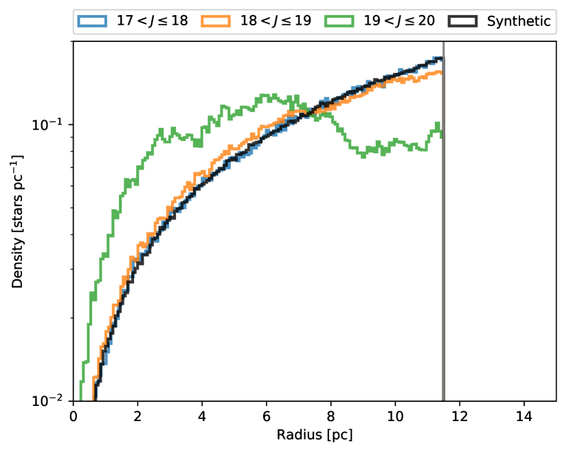
Figure 1: Density of sources in the combined DANCe+Tycho catalogue as a function of the radial distance to the cluster centre and the J magnitude. Top panel: All sources contained within the limiting magnitudes. Bottom panel: Sources within the 11.5 pc radius of spatial completeness (vertical grey line), and binned in magnitudes. The black line represents the density of two million sources uniformly distributed in the plane of the sky.

Another important constraint is the number of cluster stars observed within the survey area coverage. Truncating the probability distributions properly accounts for the cluster members left outside the truncation radius. However, due to the several artefacts surrounding the images of bright sources (e.g. halos, spikes, saturation), potential cluster members could also remain undetected. Furthermore, these artefacts can severely bias any evidence of mass segregation, as the most massive and brightest stars are located at the centre of the cluster. However, the statistical treatment of the impact of these artefacts lays beyond the scope of this work.

The information provided by the observational constraints, which we call $I$, consists of the maximum radius, $R_{max}=11.5$pc, and the number of stars observed within this radius, $N=1954$. These constraints will be incorporated into the model through the $likelihood$.

2.2 Contamination

Olivares et al. (2017) estimate a contamination rate of $4.3\pm 0.2$% in their sample of candidate members at the probability threshold of $p_{84\%}$¿ 0.84. This would amount to 84 of their 1963 candidate members. Also, Sarro et al. (2014) estimate that the contamination rate of their methodology is $11.0\pm 2.0$% for a probability threshold of $p=0.5$, similar to that used by Bouy et al. (2015) to classify the candidate members of their Tycho+DANCe data set. Thus, in our combined Tycho+DANCe list of candidate members, we acknowledge a mean contamination rate of $\sim 8\%$ (approx. 156 objects). We expect these contaminating sources to be uniformly distributed in right ascension and declination because the position on the sky was explicitly removed from the calculation of membership probabilities. Nevertheless, there may be a mild positive gradient of the density towards the Galactic centre. In addition, these contaminants may not be uniformly distributed in $J$ band, with possible concentrations around 14 and 17 mag, where the entanglement of field and cluster populations is higher. The quantification of this possible dependency of contaminants with photometric magnitude and its consequences lay beyond the objective of this work and will be analysed in future studies.

3 Spatial density models

3.1 Spherical models

In this Section we consider spherically symmetric models of the spatial distribution of Pleiades members. In the following paragraphs we give a brief description of each model, its analytical parameterisation, and the corresponding references.

Our starting point is the classical King’s profile. Although it was introduced as an empirical law to describe the number surface density of globular clusters, it has also been used to describe open clusters (see Alonso-Santiago et al. 2017; Panwar et al. 2017, for recent applications), globular clusters (Myeong et al. 2017) and even to study galaxies (Robotham et al. 2017), halo substructure (Sohn et al. 2007) and the dark matter distribution (Jiang & van den Bosch 2016). The analytical description of the surface number density of stars $n$ is given by

$$n(R)=k\cdot\left(\frac{1}{\sqrt{1+(R/r_{c})^{2}}}-\frac{1}{\sqrt{1+(r_{t}/r_{c})^{2}}}\right)^{2},$$ (1)

where $r_{c}$, the core radius, is a scale factor, $r_{t}$ is the tidal radius, and $k$ is a constant related (but not equal) to the central surface density. In the following we use $R$ instead of $r$ (as is often commonly done in the literature) to refer to the distance from the system centre projected on the celestial sphere.

In addition to the classical King’s profile we have tested two extensions of it. We define the Generalised King’s profile (hereafter GKing) as the classical King’s profile without fixing the exponents of the analytical expression. Instead of Eq. 1, we have

$$n(R)=k\cdot\left[\left(1+(R/r_{c})^{\frac{1}{\alpha}}\right)^{-\alpha}-\left(1+(r_{t}/r_{c})^{\frac{1}{\alpha}}\right)^{-\alpha}\right]^{\beta},$$ (2)

where the classical King’s profile is recovered for $\alpha=0.5$ and $\beta=2$. To the best of our knowledge, only in the work of Robotham et al. (2017) has a similarly modified King’s profile been used. However, the profile used by those authors is more restrictive than the one presented here, requiring that $\beta=\alpha^{-1}$, and that both terms $(R/r_{c})$, and $(r_{t}/r_{c})$ are at the power of 2.

The optimised generalised King’s profile (hereafter OGKing) is the GKing profile with the values of $\alpha$ and $\beta$ fixed at the maximum-a-posteriori (MAP) values of the GKing parameters. This maximises the Bayesian evidence and reduces the dimensionality of the parameter space.

To avoid the use of a tidal radius in the radial profile, we have also considered the model proposed by Elson et al. (1987), henceforth EFF, to describe young open clusters in the Large Magellanic Cloud. Their surface density (in star counts per solid angle) is given by

$$n(R)=n(0)\cdot(1+(R/r_{c})^{2})^{\frac{\gamma}{2}},$$ (3)

with $r_{c}$ the core radius, and $\gamma$ the slope of the profile at radii much larger than the core radius.

Finally, we analyse a more general parameterisation introduced in Lauer et al. (1995), Byun et al. (1996) and Zhao (1997), where the projected mass density is given as

$$\rho(R)=\frac{k^{\prime}}{(R/r_{c})^{\gamma}\cdot(1+(R/r_{c})^{1/\alpha})^{(\gamma-\beta)\alpha}}.$$ (4)

Equation 4 represents a double power law, with $r_{c}$ being the so-called core or break radius, $\gamma$ and $\beta$ the exponents of the inner and outer regions, respectively, $\alpha$ the width of the transition region, and $k^{\prime}$ a scale constant. Meaningful values of these parameters fulfil the following conditions: $\alpha>0$ and $0\leq\gamma\leq\beta$. The aforementioned works assume this functional form for the projected surface brightness, the projected mass density $\rho$, and the volume density $v$, although the latter two are related by integration:

$$\rho(R)=\int_{0}^{\infty}v(r)\cdot{\rm d}z,$$ (5)

where $z$ is the distance along the line of sight.

In this work we use the same analytical expression as in Eq. 4 but for the number density $n(R)$. We call this model the generalised density profile (hereafter GDP), as it comprises many simpler models, each of which corresponding to particular choices of the model parameters. Several density profiles proposed to describe galaxies can indeed be grouped by parameter values. For example, $\alpha=1$ includes models by Navarro et al. (1997), Hernquist (1990), Jaffe (1983), and Moore et al. (1999). Similarly, $\alpha=1/2,\gamma=0$ includes the models by Plummer (1911) (with $\beta=5$), by Sackett & Sparke (1990) and by de Zeeuw (1985). The EFF model corresponds also to $\alpha=1/2,\gamma=0$. King’s profile, however, cannot be cast into this general model unless the tidal radius $r_{t}$ is fixed at infinity.

For our spatial analysis, we also considered the restricted generalised profile (RGDP), corresponding to the generalised profile with the value $\gamma$ fixed at 0.

We note that we have used similar names for parameters $r_{c}$ and $\gamma$ in all the aforementioned formulations. However, these parameters do not share the same meaning amongst models. The latter is distinctively specified by each model relation $\mathcal{M}$.

In all cases, the $R$ coordinate is defined with respect to the cluster centre. The actual values of $R$ then depend on the choice of this origin (see Sect. 3.2).

3.2 Central symmetry constraint

In the above, we have defined six models: King, GKing, OGKing, EFF, GDP and RGDP. Each of them has a different set of parameters. For example, the King’s model depends on two parameters ($r_{c}$ and $r_{t}$), the EFF model depends on two other parameters ($r_{c}$ and $\gamma$), and the generalised profile GDP depends on four parameters ($\alpha$, $\beta$, $\gamma$ and $r_{c}$).

In reality, there are always two more parameters that do not appear explicitly in any of the above analytical formulations of the number density profiles. These are the cluster centre coordinates from which all radial distances $R$ are measured. It is not a minor question because the problem is degenerate, and there is a maximum likelihood solution for each choice of the cluster centre. In principle, one could even choose a poor cluster centre estimate that renders the angular distribution of members asymmetric, and obtain a maximum likelihood fit better than those obtained with a better centred estimate. The models assume central symmetry, but this can only be ensured approximately. There is a region of non-negligible extent, where the cluster centre may be, and any particular choice of its position will influence the posterior distribution inferred. Thus, in order to propagate appropriately this uncertainty about the cluster centre position in our posterior inferences, we have included the two cluster centre coordinates, $\alpha_{c}$ and $\delta_{c}$, as further parameters of our models (their allowed intervals will be described in Sect. 4.3).

For any given choice of the central coordinates, we calculate the radial distance, $R$, and the position angle $\theta$ of each star in our data set. To avoid biases introduced by projection effects of objects located far from the cluster centre, we project each object’s coordinates into the plane of the sky along the line-of-sight vector (see for example, Eq. 1 of van de Ven et al. 2006).

These projected coordinates are

$$\tilde{x}= \sin(\alpha-\alpha_{c})\cdot\cos(\delta),$$

$$\tilde{y}= \cos(\delta_{c})\cdot\sin(\delta)-\sin(\delta_{c})\cdot\cos(\delta)\cdot\cos(\alpha-\alpha_{c}).$$ (6)

From these projected coordinates, the radial distance, $R$, and the position angle, $\theta$, are computed as

$$R= \sqrt{\tilde{x}^{2}+\tilde{y}^{2}},$$

$$\theta= \arctan 2(\tilde{x},\tilde{y})+2\pi\ \ (\rm{mod}\ \ 2\pi).$$ (7)

The requirement of central symmetry is enforced by the inclusion of a multiplicative term in the likelihood. For a given set of parameter values of $\alpha_{c},\delta_{c}$ , we divide the computed polar angles of individual stars, $\theta$, into four symmetric quadrants (divisions at $[0,\pi/2,\pi,3\pi/2]$) and require that the number of stars in each quadrant be Poisson distributed with a mean rate given by $N_{q}=N_{tot}/4$. Under this model, the likelihood of any given proposal for the model parameters ($\alpha_{c}$, $\delta_{c}$) will be

$$\mathcal{L} =p(N_{1},N_{2},N_{3},N_{4}|\alpha_{c},\delta_{c})$$

$$=\mathcal{P}(N_{1}|N_{q})\cdot\mathcal{P}(N_{2}|N_{q})\cdot\mathcal{P}(N_{3}|N_{q})\cdot\mathcal{P}(N_{4}|N_{q}),$$ (8)

where $N_{i},i=1,2,3,4$ is the number of sources in each quadrant, and $\mathcal{P}(N_{i}|N_{q})$ is the Poisson distribution with mean rate $N_{tot}/4$ evaluated at $N_{i}$.

3.3 Elliptical models

In this Section we extend the aforementioned spherical models to allow for deviations from radial symmetry. We do this by allowing variations of the radial profile that depend on the angular coordinate but still maintain biaxial symmetry. This can be done in many ways. In this work we focus on the simplest one: the analytical expression of the radial profile is maintained along any radial direction but the profile parameters (e.g. $r_{c}$ and $r_{t}$ in the King profile) have an ellipse-like dependence on the angular coordinate.

This requires the definition of a coordinate system centred at the cluster centre (parameters $\alpha_{c}$ and $\delta_{c}$), and potentially rotated from the RA-Dec system of axes. Thus, we further include the angle $\phi$ between the principal axes of the ellipse and RA-Dec system as a parameter of these models. The coordinates $\tilde{x}$ and $\tilde{y}$ of Eq. 6 are rotated by angle $\phi$ to obtain coordinates $x$ and $y$. Then, $R$ and $\theta$ are computed from the latter by means of Eq. 7.

The radially symmetric parameters of the previous Section have now an angular dependency, which is now expressed by means of the characteristic radii at the semi-major and semi-minors axes (denoted by subscripts $a$ and $b$, respectively). These new radii are expressed as

$$r(\theta)=\frac{r_{a}\cdot r_{b}}{\sqrt{(r_{a}\sin(\theta))^{2}+r_{b}\cos(\theta))^{2}}},$$ (9)

where $\theta$ is the position angle measured from the semi-major axis, and $r_{a}$ and $r_{b}$ are the parameters representing the characteristic radius at the semi-major and -minor axis, respectively.

We illustrate this new biaxial dependency in the King’s profile. The surface number density is now

$$n(R)=k\cdot\left(\frac{1}{\sqrt{1+({R}/{r_{c}(\theta)})^{2}}}-\frac{1}{\sqrt{1+({r_{t}(\theta)}/{r_{c}(\theta)})^{2}}}\right)^{2},$$ (10)

where $r_{c}$ and $r_{t}$ are obtained from Eq. 9. Explicitly they are,

$$r_{c}(\theta)=\frac{r_{ca}\cdot r_{cb}}{\sqrt{(r_{ca}\sin(\theta))^{2}+r_{cb}\cos(\theta))^{2}}},$$ (11)

$$r_{t}(\theta)=\frac{r_{ta}\cdot r_{tb}}{\sqrt{(r_{ta}\sin(\theta))^{2}+r_{tb}\cos(\theta))^{2},}}$$ (12)

where $r_{ca}$ and $r_{ta}$ are the core and tidal semi-major axis of the ellipse, and $r_{cb}$ and $r_{tb}$ correspond to the semi-minor axis. We highlight that we do not constrain the two ellipses to have the same aspect ratio, but they are co-aligned.

For the other model, the surface densities are similarly obtained. We do not incorporate any angle dependence for the exponents $\alpha,\beta$ or $\gamma$.

The position angle of the semi-major axis with respect to the Right Ascension axis ($\phi$) is constrained using the equivalent of the radial symmetry likelihood term, except that now the position angle has its origin at the semi-major axis.

3.4 Segregated models

Finally, in this Section we introduce another set of profiles to revisit the problem of mass segregation in the context of the Pleiades.

We consider the previous biaxially symmetric models to which we add a dependence of the core radius with the J magnitude. We select the J magnitude because it is the reddest of the magnitudes that are available for all candidate members. We assume that stars of the same mass have approximately the same magnitude and that distance differences (due to the 3D spatial extent of the Pleiades) average out. The core radius dependence with the J magnitude is modelled as

$$r_{c}(\theta,J)=r_{c}(\theta)+\kappa\cdot(J-J_{mode}),$$ (13)

where $J_{mode}$ is the mode of the J band distribution.

The slope of the relationship, $\kappa$, is independent of the angle $\theta$. Therefore, for $J=J_{mode}=13.6$ the model reduces to the elliptic profile described in Section 5.2. A positive value of $\kappa$ corresponds to smaller values of the core radius for stars brighter than $J_{mode}=13.6$; in other words, it describes a system where the more massive stars are more concentrated than the less massive ones.

4 Bayesian analysis

As mentioned in Section 2, our data set may be contaminated. Thus, in an effort to minimise the possible impact that these contaminants may have on our inference, we also model their spatial distribution. Hence, our model of the spatial distribution of stars not only includes the model of the Pleiades cluster, but also a field component which is modelled by a uniform spatial distribution $\mathcal{U}$ within the maximum radius $R_{max}$.

The measured properties of each of star in our data set can be assumed to be unaffected by the measured properties of any other star in the data set (this assumption is called statistical independence). Under this assumption, the probability that the data set was generated by the mixture of cluster and field is the product of the probabilities that each of the stars was generated by this mixture.

Allowing $D=\{d_{i},\pi_{i}\}_{i}^{N}$ to denote our data set, with $d$ comprising the sky coordinates and $J$ magnitude, and $\pi$ the cluster membership probability of each object, the probability or likelihood of the data set $D$, given the model $\mathcal{M}$, constraints $I$, and parameters $\bm{q}$, is

$$\mathcal{L}(D|\bm{q},\mathcal{M},I)=\prod_{i}^{N}\left[\pi_{i}\cdot p(d_{i}|\bm{q},\mathcal{M},I)+(1-\pi_{i})\cdot\mathcal{U}(d_{i}|I)\right].$$ (14)

The probability $p(d|\bm{q},\mathcal{M},I)$ depends on the profile under consideration and is described in the following Section.

4.1 Probabilistic framework

To avoid the use of bins and to properly infer the parameters of the models presented in Section 3, we need to convert the projected stellar densities into probability density functions that describe the probability of finding a star between $R$ and $R+{\rm d}R$, under the assumption of spherical symmetry. The probability density function $p(R)$ is constructed from the definition:

$$p(R)\cdot{\rm d}R=\frac{2\pi\cdot R\cdot n(R)\cdot{\rm d}R}{N},$$ (15)

where $N$ is the total number of stars in the system.

This probability is renormalised to integrate to unity at the truncation radius $R_{max}$, which in our data set corresponds to 11.5 pc. Thus,

$$p_{T}(R)=\left\{\begin{array}[]{rcl}\frac{p(R)}{\int_{0}^{R_{max}}p(R)\cdot\rm{d}R}&\mbox{for}&R\leq R_{max}\\ 0&\mbox{for}&R>R_{max}\end{array}\right..$$ (16)

All the probabilities rendered by our set of models are renormalised according to the previous equation. However, in the following and for the sake of simplicity, we only present the non-truncated probabilities.

Applying Eq. 15 to the spherically symmetric King’s profile, we obtain

$$p(R)=\frac{k\cdot 2\pi}{N}\cdot R\cdot\left(\frac{1}{\sqrt{1+(R/r_{c})^{2}}}-\frac{1}{\sqrt{1+(r_{t}/r_{c})^{2}}}\right)^{2}.$$ (17)

Actually, in probabilistic inference we write this probability function as:

$$p(R|r_{c},r_{t},k_{1},I,\mathcal{M}_{1})=k_{1}\cdot R\cdot\left(\frac{1}{\sqrt{1+(R/r_{c})^{2}}}-\frac{1}{\sqrt{1+(r_{c}/r_{t})^{2}}}\right)^{2},$$ (18)

where we have defined a new constant, $k_{1}=\frac{k\cdot 2\pi}{N}$, and made explicit the dependence of the probability on the underlying analytical expression ($\mathcal{M}_{1}$), the constraints $I$, and the values of the parameter set ($k_{1},r_{c}$ and $r_{t}$). In practice, $k_{1}$ is treated as a normalisation constant (to enforce unit integral) and there is no need to know the total number of stars in the system.

For the generalised King’s profile, this becomes

$$p(R|r_{c},r_{t},\alpha,\beta,k_{2},I,\mathcal{M}_{2})=\\ k_{1}\cdot R\cdot\left[\left(1+(R/r_{c})^{\frac{1}{\alpha}}\right)^{-\alpha}-\left(1+(r_{t}/r_{c})^{\frac{1}{\alpha}}\right)^{-\alpha}\right]^{\beta}.\\$$ (19)

Likewise, the expression for the EFF model is

$$p(R|r_{c},\gamma,k_{3},I,\mathcal{M}_{3})=k_{3}\cdot R\cdot(1+(R/r_{c})^{2})^{\frac{\gamma}{2}}.$$ (20)

And finally, the GDP model is given by

$$p(R|r_{c},\alpha,\beta,\gamma,k_{4},I,\mathcal{M}_{4})=\frac{k_{4}\cdot R}{(R/r_{c})^{\gamma}\cdot(1+(R/r_{c})^{1/\alpha})^{(\gamma-\beta)\alpha}},$$ (21)

with $\gamma=0$ for the RGDP model.

For the elliptical and luminosity segregated density profiles, the likelihoods are obtained similarly by adding $\phi$ and replacing $r_{c}$ and $r_{t}$ by $r_{ca},r_{cb}$ and $r_{ta},r_{tb}$ in the model parameters, and introducing the dependence on $\theta$ and $J$ in the relations. For example, the likelihood of the biaxial King’s profile is

$$p(R,\theta|\phi,r_{ca},r_{cb},r_{ta},r_{tb},k_{5},I,\mathcal{M}_{5})=\\ k_{5}\cdot R\cdot\left(\frac{1}{\sqrt{1+({R}/{r_{c}(\theta)})^{2}}}-\frac{1}{\sqrt{1+({r_{t}(\theta)}/{r_{c}(\theta)})^{2}}}\right)^{2}\,.$$ (22)

4.2 Model selection

In this Section we aim at comparing the aforementioned analytical parametrizations of the projected stellar densities in the light of the currently available data. In order to do so, we use the Bayesian evidence, also known as marginal likelihood. In the following, we use evidence (and its plural evidences) to refer to the Bayesian evidence. The evidence is the key for model comparison in the Bayesian framework. In this framework, the model comparison is done on the basis of the model posterior probability $p(\mathcal{M}|D)$. This is the probability of model $\mathcal{M}$ given the collected data $D$. In our opinion, this is the most natural way to compare and select (if needed) models in the scientific context. The posterior probability can be expressed as

$$p({\mathcal{M}}|D)=\frac{p(D|{\mathcal{M}})\cdot p({\mathcal{M}})}{p(D)},$$ (23)

using Bayes’ theorem. The ratio of posterior probabilities can then be expressed as

$$\frac{p({\mathcal{M}}_{i}|D)}{p({\mathcal{M}}_{j}|D)}=\frac{p(D|{\mathcal{M}}_{i})}{p(D|{\mathcal{M}}_{j})}\cdot\frac{p({\mathcal{M}}_{i})}{p({\mathcal{M}}_{j})}.$$ (24)

If there is no difference in the prior probabilities for models $i$ and $j$, then the posterior ratio is equal to the marginal likelihood ratio (also known as Bayes Factor), where the marginal likelihood (i.e. the evidence) is the full likelihood marginalised over the model parameters q, as follows

$$p(D|{\mathcal{M}})=\int p(D|\bf{q},{\mathcal{M}})\cdot{\rm d}\bf{q}.$$ (25)

It is important to remark that the Bayesian model comparison naturally incorporates a preference towards the less complex models if they are equally supported by the data. In fact, the preference is towards models with less effective parameters (understood as parameters that the data can constrain).

The computation of the posterior probability distributions and the evidence of each model is carried out in practice using the Nested Sampling (Skilling 2006) algorithm as implemented in PyMultiNest (Buchner et al. 2014).

4.3 Priors

In the spherical models, we have assumed exponential priors, with a scale value of 1, and truncated at 100, for all exponent parameters $\alpha,\beta,\gamma$, normal priors for the central coordinates (with mean at $[56.65^{\circ},24.13^{\circ}]$ and standard deviation of one degree), and Half-Cauchy priors for radial parameters (with scale parameter at 10 pc). These priors fall in the category of weakly informative ones (see Gelman 2006).

In the biaxially symmetric models, we use the same priors as for the radially symmetric ones but we restrict the semi-major axes of the core and tidal radii to be larger than, or at least equal to, their corresponding semi-minor axis. We also include a uniform prior for the angle $\phi\in[-\pi/2,\pi/2]$.

In the luminosity segregated models, in addition to the previous priors, we use a normal, $\mathcal{N}(0,0.5)$, as a prior for $\kappa$, which represents our prior beliefs of almost negligible luminosity segregation.

The code to perform the analysis of the present work, together with the data set described in Section 2, is available at https://github.com/olivares-j/PyAspidistra

5 Results and Discussion

We apply the Bayesian formalism described in Section 4 to the data set detailed in Section 2. Thus, for each of our models we obtain the posterior distribution of its parameters, together with its evidence. Appendix B contains the details of the inferred posterior distributions, figures of the fitted densities and marginal distributions, together with the uncertainties of the parameters in each analysed model. Table 2 summarises the evidences and Bayes Factors resulting from all our models and their extensions. In the following we use these evidences to discuss the model comparison.

The boundaries for decision making from Bayes Factors should be set ab initio. We mostly discuss our results following the classical scale by Jeffreys (1961). In this scale, the strength of the evidence is said to be: Inconclusive if the Bayes Factor is $\lesssim$ 3:1, weak if it is $\sim$ 3:1, moderate if it is $\sim$12:1, and strong if it is $\gtrsim$ 150 :1. Nevertheless, we hope that our conclusions can be shared by the reader independently of the scale used to categorise the Bayes Factors.

Table 2: Natural logarithm of the evidence for each profile density (diagonal) and Bayes factors (off-diagonal elements, with the evidence for the model specified in the column header placed in the denominator, i.e. $p(D|\mathcal{M}_{row})/p(D|\mathcal{M}_{column})$). The evidence corresponds to the data set truncated at 11.5pc.

		Radial						Biaxial						Segregated
		EFF	GDP	GKing	King	OGKing	RGDP	EFF	GDP	GKing	King	OGKing	RGDP	EFF	GDP	GKing	King	OGKing	RGDP
Radial	EFF	-4569.15	8.83	0.83	0.40	0.19	2.53	¡1e-2	¡1e-2	¡1e-2	¡1e-2	¡1e-2	¡1e-2	¡1e-2	¡1e-2	¡1e-2	¡1e-2	¡1e-2	¡1e-2
	GDP	0.11	-4571.33	0.09	0.05	0.02	0.29	¡1e-2	¡1e-2	¡1e-2	¡1e-2	¡1e-2	¡1e-2	¡1e-2	¡1e-2	¡1e-2	¡1e-2	¡1e-2	¡1e-2
	GKing	1.21	10.64	-4568.97	0.48	0.23	3.05	¡1e-2	¡1e-2	¡1e-2	¡1e-2	¡1e-2	¡1e-2	¡1e-2	¡1e-2	¡1e-2	¡1e-2	¡1e-2	¡1e-2
	King	2.51	22.17	2.08	-4568.23	0.49	6.35	¡1e-2	¡1e-2	¡1e-2	¡1e-2	¡1e-2	¡1e-2	¡1e-2	¡1e-2	¡1e-2	¡1e-2	¡1e-2	¡1e-2
	OGKing	5.13	45.31	4.26	2.04	-4567.52	12.99	¡1e-2	¡1e-2	¡1e-2	¡1e-2	¡1e-2	¡1e-2	¡1e-2	¡1e-2	¡1e-2	¡1e-2	¡1e-2	¡1e-2
	RGDP	0.40	3.49	0.33	0.16	0.08	-4570.08	¡1e-2	¡1e-2	¡1e-2	¡1e-2	¡1e-2	¡1e-2	¡1e-2	¡1e-2	¡1e-2	¡1e-2	¡1e-2	¡1e-2
Biaxial	EFF	¿999	¿999	¿999	¿999	¿999	¿999	-4557.32	5.14	0.08	0.08	0.01	0.84	¡1e-2	¡1e-2	¡1e-2	¡1e-2	¡1e-2	¡1e-2
	GDP	¿999	¿999	¿999	¿999	¿999	¿999	0.19	-4558.96	0.02	0.02	¡1e-2	0.16	¡1e-2	¡1e-2	¡1e-2	¡1e-2	¡1e-2	¡1e-2
	GKing	¿999	¿999	¿999	¿999	¿999	¿999	12.31	63.26	-4554.81	0.97	0.13	10.37	¡1e-2	0.01	¡1e-2	¡1e-2	¡1e-2	¡1e-2
	King	¿999	¿999	¿999	¿999	¿999	¿999	12.64	64.93	1.03	-4554.78	0.14	10.64	¡1e-2	0.01	¡1e-2	¡1e-2	¡1e-2	¡1e-2
	OGKing	¿999	¿999	¿999	¿999	¿999	¿999	91.95	472.37	7.47	7.28	-4552.80	77.41	0.04	0.10	¡1e-2	¡1e-2	¡1e-2	0.04
	RGDP	¿999	¿999	¿999	¿999	¿999	¿999	1.19	6.10	0.10	0.09	0.01	-4557.15	¡1e-2	¡1e-2	¡1e-2	¡1e-2	¡1e-2	¡1e-2
Segregated	EFF	¿999	¿999	¿999	¿999	¿999	¿999	¿999	¿999	212.43	206.96	28.45	¿999	-4549.45	2.95	0.10	0.03	0.16	1.15
	GDP	¿999	¿999	¿999	¿999	¿999	¿999	886.29	¿999	71.98	70.13	9.64	746.15	0.34	-4550.53	0.03	0.01	0.05	0.39
	GKing	¿999	¿999	¿999	¿999	¿999	¿999	¿999	¿999	¿999	¿999	293.70	¿999	10.32	30.47	-4547.12	0.32	1.64	11.86
	King	¿999	¿999	¿999	¿999	¿999	¿999	¿999	¿999	¿999	¿999	913.86	¿999	32.12	94.81	3.11	-4545.98	5.10	36.91
	OGKing	¿999	¿999	¿999	¿999	¿999	¿999	¿999	¿999	¿999	¿999	179.23	¿999	6.30	18.59	0.61	0.20	-4547.61	7.24
	RGDP	¿999	¿999	¿999	¿999	¿999	¿999	¿999	¿999	184.89	180.13	24.76	¿999	0.87	2.57	0.08	0.03	0.14	-4549.59

5.1 Models with radial symmetry

The upper-left panel of Table 2 summarises the evidences and Bayes Factors obtained from our radially symmetric models. In addition, Table 3 shows the Maximum-a-Posteriori (MAP) estimate of each parameter in the radially symmetric models (uncertainties are shown in the Appendix B in the form of covariance matrices).

Table 3: Maximum-a-posteriori estimates of the inferred parameters in each radially symmetric model.

	$\alpha_{c}$ [∘]	$\delta_{c}$ [∘]	$r_{c}$ [pc]	$r_{t}$ [pc]	$\alpha$	$\beta$	$\gamma$
EFF	56.66	24.18	2.23				2.53
GDP	56.66	24.17	3.02		0.64	2.95	0.09
GKing	56.66	24.16	1.42	18.17	0.46	1.48
King	56.66	24.16	2.04	32.08
OGKing	56.66	24.17	1.38	18.87
RGDP	56.66	24.17	3.11		0.69	3.13

We observe that the evidences cluster in two groups. On one hand there is the family of King’s models, where the evidence to compare between them is inconclusive and weak in favour of OGKing over GKing. On the other hand there are the EFF, GDP, and RGDP, where there is weak evidence supporting EFF over GDP and RGDP. There is inconclusive evidence supporting RGDP over GDP.

Comparing the two groups shows that models in King’s family provide evidence that is: inconclusive and weak over the EFF, weak and moderate over RGDP, and moderate over GDP. Using this information only, we conclude that the tidal radius is an important parameter.

In addition, we observe that in GDP and RGDP, parameters $r_{c}$ and $\beta$ show large correlations (0.85 and 0.92 for GDP and RGDP, respectively) and are relatively unconstrained with large uncertainties; see Appendix B. Despite this fact, the models still provide evidences comparable to those of the other models, suggesting that these two parameters, although necessary for the model, are unconstrained by the data, and therefore not penalised by the evidence. Aiming at eliminating this source of degeneracy, we tested models in which one of these two parameters was removed. However, the fits and evidence resulting from them were poorer than that of the RGDP. Thus, we consider these parameters as necessary for this model.

We find that the introduction of more flexibility in the analytical expressions of the classical radially symmetric profiles does not provide an increased amount of evidence, and results, in some cases, in unconstrained parameters and a loss of the interpretability associated to the original formulations. Therefore, the competing models are within the King’s family, with insufficient evidence to select amongst them. Only additional, perfectly acceptable prejudices like physical interpretability or the ability to compare with previous results can be invoked to choose one (e.g. King’s profile) over the rest.

The Bayes Factors seem to indicate (with inconclusive evidence however) that the best model is the OGKing. However, the fact that this profile has a larger evidence than any of the remaining models should come as no surprise since it results from fixing the values of $\alpha$ and $\beta$ of the GKing model to their MAP values.

Comparing the rest of the models, we see that the poorest model is GDP with moderate evidence against it. The best models are again in King’s family, followed by EFF and RGDP.

The conclusion from the comparison of these radially symmetric profiles is that i) there is no compelling reason to abandon the widely used King profile, and ii) there are slightly better models, but we lack evidence to prove if they truly represent a requirement to make the King’s profile more flexible to accommodate the data.

5.2 Biaxially symmetric models

The central panel of Table 2 contains the logarithm of the evidences and Bayes Factors of the biaxially symmetric models. The evidences follows a pattern similar to that observed for the radially symmetric models, with the exception of those that are against the GDP model. We can conclude that there is strong evidence for the family of King’s models and against the GDP one. The evidence is still moderate and too weak to compare the rest of the models.

Additionally, we compute a posteriori (from the MCMC chains) the ellipticities $\epsilon_{rc}$ and $\epsilon_{rt}$, which are defined as,

$$\epsilon_{rc}=1-\frac{r_{cb}}{r_{ca}},$$

$$\epsilon_{rt}=1-\frac{r_{tb}}{r_{ta}},$$

with the latter available only for the King’s family of models.

Table 4: Maximum-a-posteriori estimates of the inferred parameters in each biaxially symmetric model. Ellipticities are derived a posteriori using the inferred parameters.

	$\alpha_{c}$ [∘]	$\delta_{c}$ [∘]	$\phi$ [rad]	$r_{ca}$ [pc]	$r_{ta}$ [pc]	$r_{cb}$ [pc]	$r_{tb}$ [pc]	$\alpha$	$\beta$	$\gamma$	$\epsilon_{rc}$	$\epsilon_{rt}$
EFF	56.66	24.15	0.99	2.61		2.11				2.58	0.22
GDP	56.64	24.15	1.01	3.90		3.14		0.68	3.28	0.04	0.23
GKing	56.66	24.14	0.94	1.35	18.00	1.21	12.79	0.48	1.34		0.10	0.30
King	56.64	24.20	1.01	2.05	51.23	2.04	20.92				0.07	0.64
OGKing	56.68	24.16	1.04	1.51	22.63	1.38	14.54				0.09	0.36
RGDP	56.68	24.17	0.96	4.05		3.04		0.78	3.32		0.24

Table 4 shows the MAP estimate for the parameters in the models of this Section, together with the mode of the distributions of ellipticities. Uncertainties for the latter are given in Appendix B.

We can observe that models with no tidal radius have similar $\epsilon_{rc}$ ellipticities with a mean value of $0.23\pm 0.01$. This value is similar to the 0.17 found by Raboud & Mermilliod (1998), who use a multicomponent analysis to derive the directions (although its value is not given) and the aspect ratio of the ellipse’s axes. However, it is very interesting to see that the models within King’s family result in lower values of the ellipticity in the central region and larger values in the outer one. This result is expected from the interaction with the galactic potential and is predicted by numerical simulations of open clusters (see, e.g. Terlevich 1987).

By comparing the evidences of the biaxially symmetric models to those of the radially symmetric ones, we can conclude that in all cases there is strong evidence in favour of the biaxial models.

5.3 Models with luminosity segregation

The lower-right panel of Table 2 summarises the evidences and Bayes Factors of models with luminosity segregation. Also, Table 5 shows the MAP of the inferred distributions for this set of models, together with the derived ellipticities.

Table 5: Maximum-a-posteriori estimates of the inferred parameters in each luminosity segregated model. Ellipticities are derived a posteriori using the inferred parameters.

	$\alpha_{c}$ [∘]	$\delta_{c}$ [∘]	$\phi$ [rad]	$r_{ca}$ [pc]	$r_{ta}$ [pc]	$r_{cb}$ [pc]	$r_{tb}$ [pc]	$\alpha$	$\beta$	$\gamma$	$\kappa$ [pc mag-1]	$\epsilon_{rc}$	$\epsilon_{rt}$
EFF	56.66	24.16	1.02	2.65		2.22				2.60	0.12	0.18
GDP	56.68	24.17	1.01	3.60		3.19		0.63	3.14	0.13	0.23	0.18
GKing	56.66	24.16	0.83	1.39	16.88	1.22	12.61	0.67	1.28		0.13	0.05	0.38
King	56.62	24.19	0.96	2.34	38.49	2.37	20.49				0.19	0.05	0.60
OGKing	56.61	24.17	0.99	1.62	22.08	1.59	14.04				0.10	0.07	0.36
RGDP	56.62	24.17	0.96	3.78		3.35		0.73	3.34		0.24	0.19

We observe that the ellipticities follow the same pattern as those of the previous Section. This is expected because we explicitly model the luminosity segregation as independent of the position angle.

The luminosity segregation inferred here is non negligible with $\kappa$ in the range 0.1 to 0.25 $\rm{pc}\,\rm{mag}^{-1}$, thus indicating that it is indeed an important parameter. However, in all the models, the marginal posterior distribution of $\kappa$ does not discard the zero value (see the marginal posterior of $\kappa$ in Appendix B).

The evidences provided by the models with luminosity segregation follow a similar pattern as those from radial symmetry. However, in this case the best model is the classical King’s, which shows only moderate evidence against the EFF, RGDP, and GDP models. The evidence of King’s model over GKing and OGKing is weak.

The evidences provided by the luminosity segregated models lead to them being strongly favoured over the radially and biaxially symmetric ones in all cases. We can conclude that, despite having a small value of $\kappa,$ the luminosity segregation is an important parameter regardless of the model used.

5.4 Total mass and number of members

In this Section we use the inferred values of the parameters in King’s family of models to derive simple estimates of the total number of members and mass of the Pleiades cluster.

For each model and extension within the King’s family, we estimate the total number of cluster members by integrating the surface density profile until the tidal radii inferred for the model. This is done for each set of parameters returned by PyMultiNest. The resulting distributions of the total numbers fore each model and extension in the King’s familly are shown in Fig. 2. Additionally, Table 6 shows the mode of these distributions. As can be seen from this Table, our current data set (with 1954 members), although twice as large as previous studies in the literature, still lacks almost one fifth of the predicted number of objects in the cluster.

Table 6: Mode of the distribution of total number of stars in the cluster.

	GKing	King	OGKing
Ctr	2087	2251	2086
Ell	2209	2509	2257
Seg	2272	2455	2231

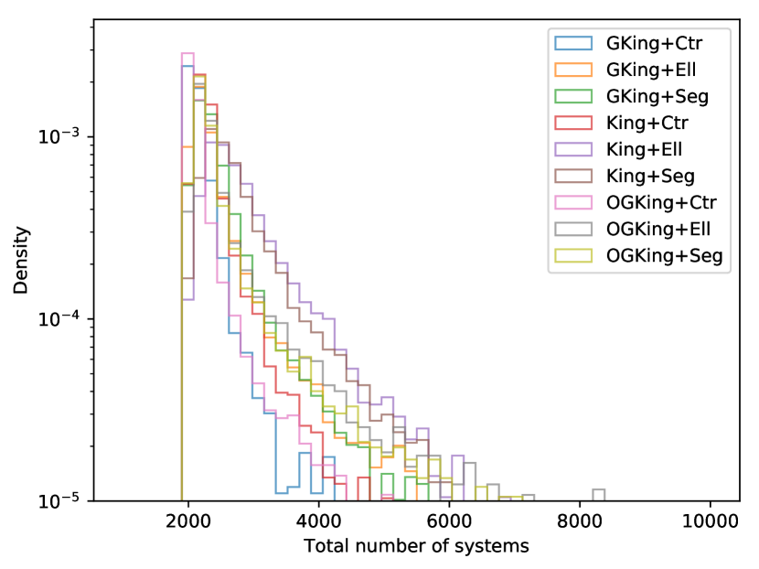
Figure 2: Distribution of the total number of systems within the tidal radius in each model and extension of the King’s family. The abbreviations Ctr, Ell, and Seg stand for the radial and biaxial symmetric models, and those with luminosity segregation, respectively.

We also estimated the total mass of the cluster using the posterior samples of the parameters returned by PyMultiNest. To gain an estimate of the total mass we use the tidal force resulting from the interaction of the self-gravitating cluster with the galactic potential. A detailed derivation of the Jacobi radius under the Hill’s approximation can be found at p. 681 of Binney & Tremaine (2008). Following the mentioned authors, the Jacobi radius is given by,

$$r_{J}=\left(\frac{Gm}{4\Omega_{0}A_{0}}\right)^{1/3},$$ (26)

where $G$ is the gravitational constant, $m$ the total mass of the cluster, and $\Omega_{0}$ the circular frequency of the cluster around the galactic centre, which can be expressed in terms of the Oort’s constants $A_{0}$ and $B_{0}$ as $\Omega_{0}=A_{0}-B_{0}$.

In the following, we assume an over-simplistic correspondence between the tidal radius of the King’s family of models and Jacobi radius. Binney & Tremaine (2008, p. 677) provide a detailed list of reasons why this correspondence is only approximate. Thus, using the Oort’s constant values given by Bovy (2017, $A=15.3\pm 0.4\,\rm{kms}^{-1}\rm{kpc}^{-1}$ and $B=-11.9\pm 0.4\,\rm{kms}^{-1}\rm{kpc}^{-1}$), we can derive an estimate of the total mass of the cluster for each inferred value of the tidal radius.

Figure 3 shows the distributions of the total mass derived from the posterior distributions of the parameters of the King’s family of models with biaxial symmetry and luminosity segregation (the distributions of total mass resulting from the radial and biaxial models are shown in Appendix B). As a summary, Table 7 shows the mode of each of these total mass distributions.

As can be seen from this Figure and Table, inferring the total mass by means of the poorly constrained tidal radius leads to large uncertainties and probably biased estimators. This effect has already been observed by Raboud & Mermilliod (1998), who derived a total mass of 4000 M_⊙ with a confidence interval ranging from 1600 M_⊙ to 8000 M_⊙. These values are in good agreement with the ones reported in Table 7 and observed in Fig. 3.

Given the large ellipticity of the cluster, we also investigated the possibility of deriving the total mass by means of the tidal elongation effect. However, the values determined are even more poorly constrained than those determined using Eq. 26.

The results of this Section show that: i) there is still a large fraction (up to 20%) of cluster members that lay beyond the spatial coverage of our data set, and, ii) although poorly unconstrained, the distributions of the total mass of the cluster seem to suggest that it is highly unlikely that the total mass of the cluster lays below the 1000 M_⊙ limit, as commonly stated in the literature. However, the large and unconstrained mass distribution could also be an artefact resulting from: i) the poor correspondence between the Jacobi radius and the tidal radius, ii) the poorly constrained values of the tidal radius, and iii) dynamical effects not taken into account to derive Eq. 26 (e.g. the cluster is not a point mass but a self gravitating and rotating system).

Table 7: Mode of the distribution of total mass of the cluster. Units in solar masses.

	GKing	King	OGKing
Ctr	1408	8584	2277
Ell	1956	6049	3571
Seg	2247	6605	3508

Figure 3: Distribution of the total mass of the cluster derived from each biaxially symmetric and luminosity segregated model of the King’s family.

6 Conclusions

In this work we have formulated the existing radially symmetric alternatives for the spatial distribution of stars in open clusters in a probabilistic framework. The set of distributions reviewed include i) the classical King’s profile with two variants put forward by us, ii) the EFF model, and, iii) a general profile inspired by galactic profiles together with a more restricted version of it. We have used Bayesian techniques to both obtain posterior probability distributions for the parameters, and evidences for each model. With them, we compare and select the best model, given the data (and its possible biases). Furthermore, we have computed Bayes Factors for all pairwise model comparisons. Due to high correlations among their $r_{c}$ and $\beta$ parameters, the GDP and RGDP models loose their physical interpretability. The result of the comparison amongst models with radial symmetry is that the King’s family of models is only mildly superior, with weak and moderate evidence, to those models without the tidal radius parameter.

Furthermore, we have analysed biaxially symmetric extensions of our set of models. The results indicate that deviations from spherical symmetry have strong evidence when compared to the more simple radially symmetric models. Additionally, the distribution of ellipticities derived from the EFF, GDP, and RGDP models peak at $0.22\pm 0.01$, which is similar to the value of 0.17 found by (Raboud & Mermilliod 1998). Within the King’s family, the models return ellipticities that are small (mean $\epsilon_{rc}=0.07\pm 0.02$) and large (mean $\epsilon_{rt}=0.44\pm 0.14$) in the inner and outer parts of the cluster, respectively. This effect is expected from the dynamical interaction of the cluster with the galactic potential, and is also predicted by numerical simulations.

We use Bayesian model selection with Bayes Factors to analyse mass segregation. We prefer to remain in the domain of direct observables and study potential differences in the parameters of the spatial distribution as a function not of mass, but of the apparent J-band magnitude. The Bayes Factors show strong evidence in favour of the luminosity segregated models, and against the simpler biaxially symmetric ones. We interpret this result as strong evidence for mass segregation.

The above conclusions heavily depend on the sample of Pleiades members selected for the analysis. In our probabilistic analysis we took into account the possibility that our sample is contaminated, but a $J$-band-dependent contamination rate ($J$-band contamination gradient) could mimic a mass segregation such as the one observed here. In addition, the halos and artefacts in the images of the central and bright stars can induce a spatial incompleteness that could also artificially enhance the slope of the luminosity segregation. Thus, our results must be taken with care. In the near future, we expect to conduct similar studies given the more homogenous and well characterised data sets (e.g. new releases of Gaia’s data).

Although the the GKing and OGKing models introduced here have greater evidences and fitting properties than the classical King’s profile, there is no strong evidence supporting an abandonment of the latter. Nevertheless, the GKing profile is a good alternative to the King’s classical profile and should be compared with it in light of new and more complete data sets.

From the model selection process, we can conclude that the classical King’s profile extended to include biaxial symmetry and mass/luminosity segregation should be the starting point in future analyses of the spatial distribution of open clusters.

Finally, we use the posterior distributions of the parameters in King’s model family to obtain rough estimates of the total mass and number of systems in the cluster. We observe that even the largest census of candidate members (Bouy et al. 2015; Olivares et al. 2017) may lack up to 20% of the predicted number of stellar systems. The probability distribution function of the cluster total mass, which is determined using approximations of the tidal force exerted by the galactic and cluster potentials, reveals that it is highly unlikely that the true cluster total mass lays below the 1000 M_⊙ limit.

The results of this work suggest that, although the Pleiades cluster is one of the most studied in the literature, the daughters of Atlas still keep many of their secrets within the oceans of the sky; probably awaiting the arrival of the final Gaia’s data.

Appendix A Effects of truncation on King’s profile.

Statistical truncation occurs when an unknown number of sources lay beyond a threshold value. This threshold value can originate in the measuring process or in the post-processing of the data. The resulting data set does not contain any information about objects beyond the threshold.

Performing inference on truncated data can bias the recovered parameters if the truncation mechanism is not included in the analysis. Nevertheless, bias can still appear if poor statistics are used to summarise the results. Practically speaking, if the truncation is too restrictive it could also lead to bias due to a reduced sample size. To estimate the impact of these effects, we generated synthetic data sets from the King’s profile, at true values of $r_{c}=2.0$ pc and $r_{t}=20.0$ pc, and infer the parameters under different sample sizes (1000,2000, and 3000 objects) and truncation radii (5,10,15,20 pc). We repeat each estimation ten times to account for randomness in the sample. Figure 4 shows the posterior distributions inferred at each sample size and truncation radius. As can be seen, accounting for truncation results in posterior distribution that correctly recovers the true parameter values. However, due to the large asymmetry in the posterior distributions of the tidal radius at the lower truncation radius (5 pc), the Maximum A Posteriori (MAP) statistic can be severely biased. Figure 5 shows the mean relative error of this statistic as a function of the truncation radius. As can be seen, the larger biases appear at the extreme case where the truncation radius is only one fourth of the true tidal radius. We note that although the MAP estimates of each of the ten realisations are biased, estimates are made in a similar way above and below the true value; except at the truncation radius of 5 pc, where they slightly over estimate the value. Also, the MAP is unbiased above truncation radii of half the tidal radius, in spite of the number of stars (at least for the tested values).

This example shows that the inference of the parameters in the King’s profile can be biased even after truncation has been accounted for. In particular, the tidal radius can be severely affected by truncation radius below one half of the tidal radius. Since this phenomenon is observed under the weakly informative priors used (half-cauchy centred at zero and scale parameter of 100), this effect can be generalised to any maximum-likelihood estimator, the $\chi^{2}$ statistic particularly.

Finally, as can be seen in Fig. 6, inferring King’s profile parameters without properly accounting for truncation leads to even larger biases.

Figure 4: Mixture of the ten posterior distributions of the core and tidal radius ($r_{c}$ and $r_{t}$, respectively) inferred under different sample sizes (line styles) and truncation radii (colours). The true parameter values are shown with the vertical grey lines.

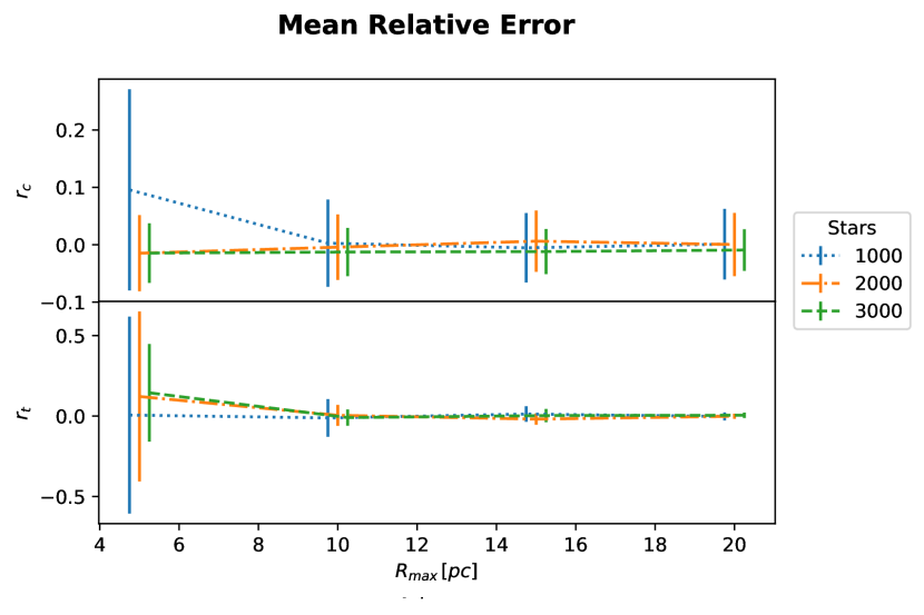
Figure 5: Mean relative error ($r_{c}$ and $r_{t}$, respectively) of the MAP statistic inferred from ten random realisations of different sample sizes (line styles) and truncation radii (colours). The uncertainties correspond to the standard deviation of the ten inferred MAPs.

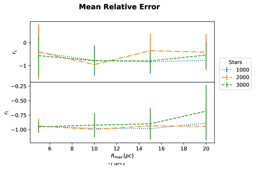
Figure 6: Mixture of the ten posterior distributions of the core and tidal radius ($r_{c}$ and $r_{t}$, respectively) inferred under different sample sizes (line styles) and truncation radii (colours) without correcting for truncation. The true parameter values are shown with the vertical grey lines.

Appendix B Posterior distributions

This Appendix contains the details of the inference performed for each of the models and extensions presented in Section 3. It is structured in the same way as that Section. It starts with the radial models, then continues with the biaxial extensions, and finishes with the luminosity segregated ones. For each extension we give: i) the uncertainties of the MAP for each model, and, ii) Figures depicting: a) the number surface density (i.e. the number of stars per square parsec), and, b) the univariate and bivariate marginal posterior distributions obtained from PyMultiNest in the form of a corner plot (Foreman-Mackey 2016). Since the MAP is computed in the joint posterior, it does not necessarily coincides with the modes of the marginal distributions.

The MAP uncertainties and correlations are summarised by covariance matrices. These are computed using the 68.2% of samples from the MCMC that were the closest to the MAP value. They represent the $2\sigma$ uncertainties and correlations of the parameters at the vicinity of the MAP.

For the biaxial and luminosity segregated models we also give the ellipticity distributions computed a posteriori from the core and tidal (when available) semi-major and semi-minor axes resulting from the PyMultiNest samples.

Finally, this Appendix also contains the distributions of the total mass of the cluster derived from the radial and biaxial models in the King’s family.

Table 8: Covariance matrix of the radially symmetric EFF model.

	$\alpha_{c}\ \ [^{\circ}]$	$\delta_{c}\ \ [^{\circ}]$	$r_{c}$ [pc]	$\gamma$
$\alpha_{c}\ \ [^{\circ}]$	0.007	0.000	0.000	0.000
$\delta_{c}\ \ [^{\circ}]$	0.000	0.006	0.001	0.000
$r_{c}$ [pc]	0.000	0.001	0.058	0.030
$\gamma$	0.000	0.000	0.030	0.027

Table 9: Covariance matrix of the radially symmetric GDP model.

	$\alpha_{c}\ \ [^{\circ}]$	$\delta_{c}\ \ [^{\circ}]$	$r_{c}$ [pc]	$\alpha$	$\beta$	$\gamma$
$\alpha_{c}\ \ [^{\circ}]$	0.012	0.000	0.004	0.000	0.002	0.000
$\delta_{c}\ \ [^{\circ}]$	0.000	0.012	0.006	0.002	0.006	-0.001
$r_{c}$ [pc]	0.004	0.006	0.589	0.062	0.330	0.004
$\alpha$	0.000	0.002	0.062	0.046	0.059	-0.016
$\beta$	0.002	0.006	0.330	0.059	0.256	-0.028
$\gamma$	0.000	-0.001	0.004	-0.016	-0.028	0.028

Table 10: Covariance matrix of the radially symmetric GKing model.

	$\alpha_{c}\ \ [^{\circ}]$	$\delta_{c}\ \ [^{\circ}]$	$r_{c}$ [pc]	$r_{t}$ [pc]	$\alpha$	$\beta$
$\alpha_{c}\ \ [^{\circ}]$	0.022	0.001	0.002	-0.021	0.001	-0.000
$\delta_{c}\ \ [^{\circ}]$	0.001	0.019	0.007	0.046	-0.004	0.005
$r_{c}$ [pc]	0.002	0.007	1.376	1.469	0.126	0.317
$r_{t}$ [pc]	-0.021	0.046	1.469	19.684	-0.214	1.139
$\alpha$	0.001	-0.004	0.126	-0.214	0.364	0.027
$\beta$	-0.000	0.005	0.317	1.139	0.027	0.141

Table 11: Covariance matrix of the radially symmetric King model.

	$\alpha_{c}\ \ [^{\circ}]$	$\delta_{c}\ \ [^{\circ}]$	$r_{c}$ [pc]	$r_{t}$ [pc]
$\alpha_{c}\ \ [^{\circ}]$	0.018	0.001	0.001	-0.001
$\delta_{c}\ \ [^{\circ}]$	0.001	0.017	0.002	0.021
$r_{c}$ [pc]	0.001	0.002	0.144	-0.945
$r_{t}$ [pc]	-0.001	0.021	-0.945	37.437

Table 12: Covariance matrix of the radially symmetric OGKing model.

	$\alpha_{c}\ \ [^{\circ}]$	$\delta_{c}\ \ [^{\circ}]$	$r_{c}$ [pc]	$r_{t}$ [pc]
$\alpha_{c}\ \ [^{\circ}]$	0.011	0.001	-0.001	-0.003
$\delta_{c}\ \ [^{\circ}]$	0.001	0.010	-0.000	-0.000
$r_{c}$ [pc]	-0.001	-0.000	0.054	-0.100
$r_{t}$ [pc]	-0.003	-0.000	-0.100	1.951

Table 13: Covariance matrix of the radially symmetric RGDP model.

	$\alpha_{c}\ \ [^{\circ}]$	$\delta_{c}\ \ [^{\circ}]$	$r_{c}$ [pc]	$\alpha$	$\beta$
$\alpha_{c}\ \ [^{\circ}]$	0.014	0.000	0.003	-0.000	0.001
$\delta_{c}\ \ [^{\circ}]$	0.000	0.012	0.006	0.000	0.005
$r_{c}$ [pc]	0.003	0.006	0.804	0.089	0.466
$\alpha$	-0.000	0.000	0.089	0.051	0.061
$\beta$	0.001	0.005	0.466	0.061	0.311

(a)

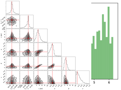
(b)

(c)

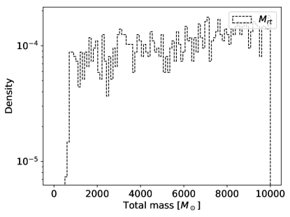
(d)

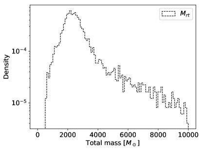
(e)

(f)

Figure 7: Inferred density of the radially symmetric profiles shown by means of the MAP value (red line) and 100 samples from the posterior distribution (grey lines). For comparison the data has been binned with Poissonian uncertainties (black dots).

Figure 9: Projections of the posterior distribution for the radially symmetric GDP model.

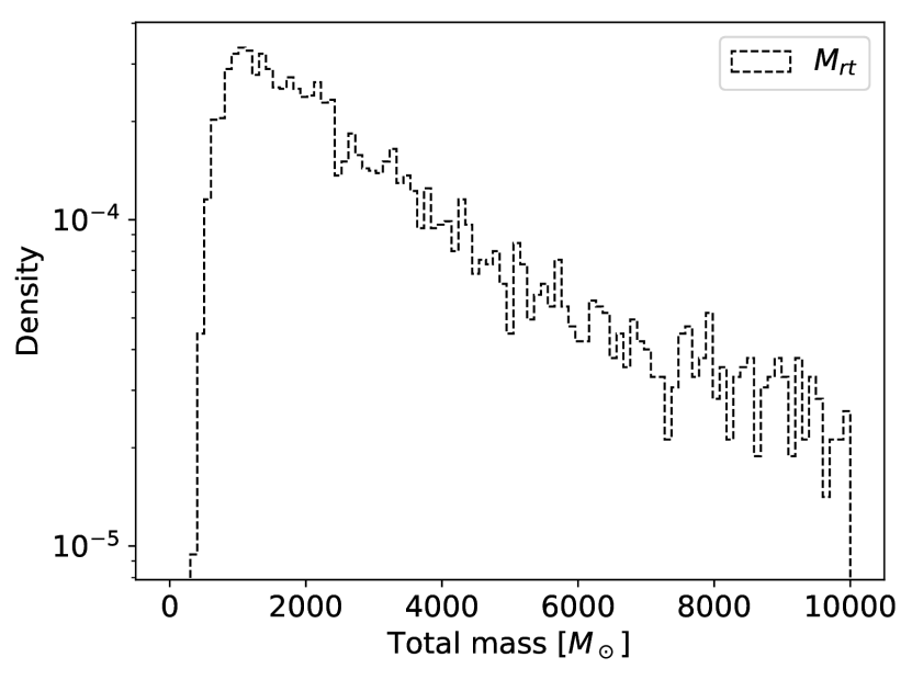
Figure 10: Projections of the posterior distribution for the radially symmetric GKing model.

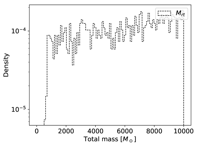
Figure 11: Projections of the posterior distribution for the radially symmetric King’s model .

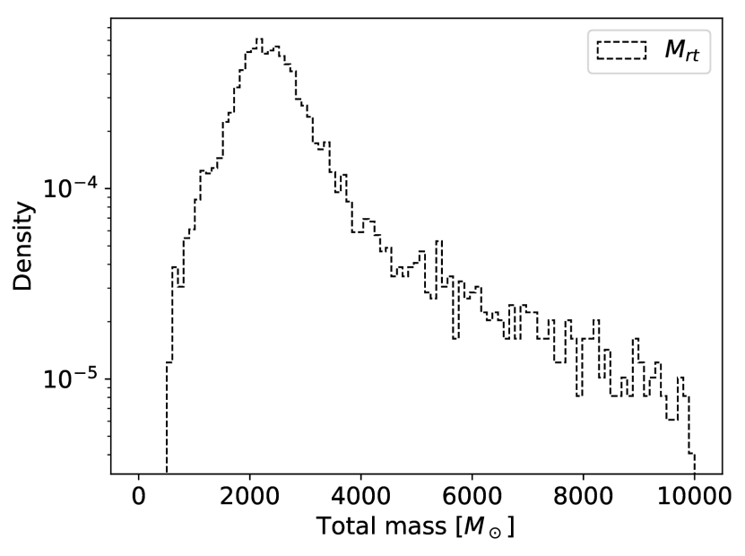
Figure 12: Projections of the posterior distribution for the radially symmetric OGKing model.

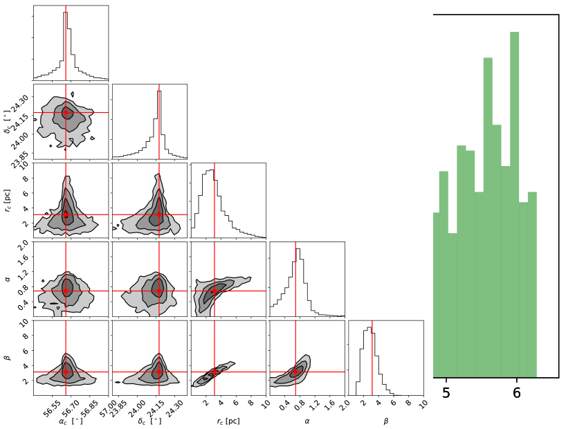
Figure 13: Projections of the posterior distribution for the radially symmetric RGDP model.

Table 14: Covariance matrix of the biaxially symmetric EFF model.

	$\alpha_{c}\ \ [^{\circ}]$	$\delta_{c}\ \ [^{\circ}]$	$\phi$ [radians]	$r_{ca}$ [pc]	$r_{cb}$ [pc]	$\gamma$
$\alpha_{c}\ \ [^{\circ}]$	0.007	-0.000	-0.001	0.000	0.000	0.000
$\delta_{c}\ \ [^{\circ}]$	-0.000	0.006	0.001	0.000	0.001	0.001
$\phi$ [radians]	-0.001	0.001	0.063	0.000	-0.002	-0.000
$r_{ca}$ [pc]	0.000	0.000	0.000	0.131	0.056	0.049
$r_{cb}$ [pc]	0.000	0.001	-0.002	0.056	0.093	0.047
$\gamma$	0.000	0.001	-0.000	0.049	0.047	0.040

Table 15: Covariance matrix of the biaxially symmetric GDP model.

	$\alpha_{c}\ \ [^{\circ}]$	$\delta_{c}\ \ [^{\circ}]$	$\phi$ [radians]	$r_{ca}$ [pc]	$r_{cb}$ [pc]	$\alpha$	$\beta$	$\gamma$
$\alpha_{c}\ \ [^{\circ}]$	0.007	-0.001	-0.001	0.002	0.000	-0.001	0.000	0.001
$\delta_{c}\ \ [^{\circ}]$	-0.001	0.005	0.001	0.005	0.005	0.002	0.005	-0.001
$\phi$ [radians]	-0.001	0.001	0.185	0.051	0.031	0.008	0.043	-0.010
$r_{ca}$ [pc]	0.002	0.005	0.051	1.204	0.801	0.101	0.547	-0.006
$r_{cb}$ [pc]	0.000	0.005	0.031	0.801	0.788	0.074	0.480	-0.009
$\alpha$	-0.001	0.002	0.008	0.101	0.074	0.044	0.070	-0.016
$\beta$	0.000	0.005	0.043	0.547	0.480	0.070	0.363	-0.033
$\gamma$	0.001	-0.001	-0.010	-0.006	-0.009	-0.016	-0.033	0.025

Table 16: Covariance matrix of the biaxially symmetric GKing model.

	$\alpha_{c}\ \ [^{\circ}]$	$\delta_{c}\ \ [^{\circ}]$	$\phi$ [radians]	$r_{ca}$ [pc]	$r_{ta}$ [pc]	$r_{cb}$ [pc]	$r_{tb}$ [pc]	$\alpha$	$\beta$
$\alpha_{c}\ \ [^{\circ}]$	0.013	-0.001	-0.004	0.001	-0.004	-0.002	-0.015	0.002	-0.001
$\delta_{c}\ \ [^{\circ}]$	-0.001	0.010	0.001	-0.002	0.014	0.004	0.005	-0.002	0.002
$\phi$ [radians]	-0.004	0.001	0.256	-0.029	0.205	0.058	-0.003	-0.022	0.027
$r_{ca}$ [pc]	0.001	-0.002	-0.029	1.587	-0.041	0.379	0.437	0.194	0.131
$r_{ta}$ [pc]	-0.004	0.014	0.205	-0.041	25.850	0.956	5.304	-0.227	0.677
$r_{cb}$ [pc]	-0.002	0.004	0.058	0.379	0.956	0.433	0.575	0.031	0.144
$r_{tb}$ [pc]	-0.015	0.005	-0.003	0.437	5.304	0.575	6.150	0.015	0.436
$\alpha$	0.002	-0.002	-0.022	0.194	-0.227	0.031	0.015	0.291	0.028
$\beta$	-0.001	0.002	0.027	0.131	0.677	0.144	0.436	0.028	0.076

Table 17: Covariance matrix of the biaxially symmetric King model.

	$\alpha_{c}\ \ [^{\circ}]$	$\delta_{c}\ \ [^{\circ}]$	$\phi$ [radians]	$r_{ca}$ [pc]	$r_{ta}$ [pc]	$r_{cb}$ [pc]	$r_{tb}$ [pc]
$\alpha_{c}\ \ [^{\circ}]$	0.019	-0.000	-0.004	0.002	-0.057	0.002	0.001
$\delta_{c}\ \ [^{\circ}]$	-0.000	0.015	0.007	-0.010	0.094	0.001	-0.001
$\phi$ [radians]	-0.004	0.007	0.359	-0.124	1.582	0.010	-0.190
$r_{ca}$ [pc]	0.002	-0.010	-0.124	1.428	-6.175	0.074	-1.548
$r_{ta}$ [pc]	-0.057	0.094	1.582	-6.175	371.812	-1.108	23.841
$r_{cb}$ [pc]	0.002	0.001	0.010	0.074	-1.108	0.154	-1.157
$r_{tb}$ [pc]	0.001	-0.001	-0.190	-1.548	23.841	-1.157	53.033

Table 18: Covariance matrix of the biaxially symmetric OGKing model.

	$\alpha_{c}\ \ [^{\circ}]$	$\delta_{c}\ \ [^{\circ}]$	$\phi$ [radians]	$r_{ca}$ [pc]	$r_{ta}$ [pc]	$r_{cb}$ [pc]	$r_{tb}$ [pc]
$\alpha_{c}\ \ [^{\circ}]$	0.009	-0.001	-0.000	-0.001	-0.006	-0.001	-0.002
$\delta_{c}\ \ [^{\circ}]$	-0.001	0.007	0.002	-0.004	0.011	0.001	-0.002
$\phi$ [radians]	-0.000	0.002	0.194	-0.031	0.166	0.009	-0.121
$r_{ca}$ [pc]	-0.001	-0.004	-0.031	0.248	-0.462	0.011	-0.080
$r_{ta}$ [pc]	-0.006	0.011	0.166	-0.462	14.223	-0.095	-0.391
$r_{cb}$ [pc]	-0.001	0.001	0.009	0.011	-0.095	0.059	-0.176
$r_{tb}$ [pc]	-0.002	-0.002	-0.121	-0.080	-0.391	-0.176	3.509

Table 19: Covariance matrix of the biaxially symmetric RGDP model.

	$\alpha_{c}\ \ [^{\circ}]$	$\delta_{c}\ \ [^{\circ}]$	$\phi$ [radians]	$r_{ca}$ [pc]	$r_{cb}$ [pc]	$\alpha$	$\beta$
$\alpha_{c}\ \ [^{\circ}]$	0.010	-0.001	-0.003	0.003	-0.000	-0.000	-0.000
$\delta_{c}\ \ [^{\circ}]$	-0.001	0.008	0.001	0.006	0.005	0.001	0.004
$\phi$ [radians]	-0.003	0.001	0.208	0.037	0.030	0.001	0.029
$r_{ca}$ [pc]	0.003	0.006	0.037	1.320	0.864	0.115	0.590
$r_{cb}$ [pc]	-0.000	0.005	0.030	0.864	0.823	0.084	0.507
$\alpha$	-0.000	0.001	0.001	0.115	0.084	0.045	0.062
$\beta$	-0.000	0.004	0.029	0.590	0.507	0.062	0.355

(a)

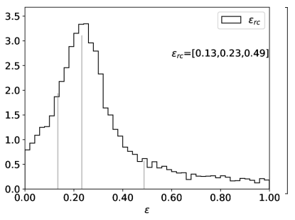
(b)

(c)

(d)

(e)

(f)

Figure 14: Inferred density of the biaxially symmetric profiles shown by means of the MAP value (red line) and 100 samples from the posterior distribution (grey lines). For comparison the data has been binned with Poissonian uncertainties (black dots).

Figure 15: Projections of the posterior distribution for the biaxially symmetric EFF model .

Figure 16: Projections of the posterior distribution for the biaxially symmetric GDP model .

Figure 17: Projections of the posterior distribution for the biaxially symmetric GKing model.

Figure 18: Projections of the posterior distribution for the biaxially symmetric King’s model.

Figure 19: Projections of the posterior distribution for the biaxially symmetric OGKing model.

Figure 20: Projections of the posterior distribution for the biaxially symmetric RGDP model.

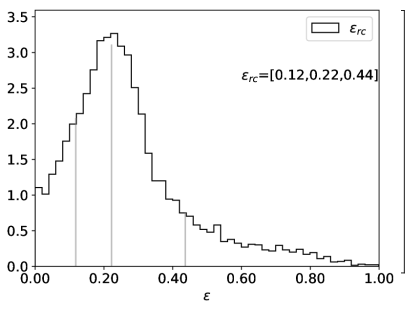
(a)

(b)

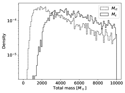
(c)

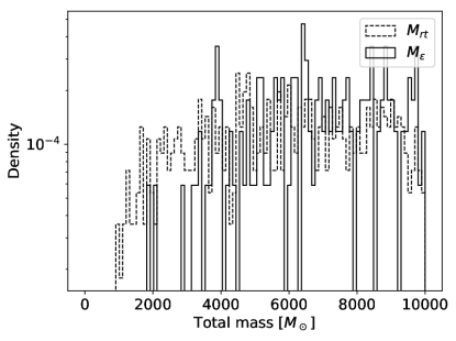
(d)

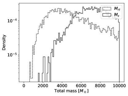
(e)

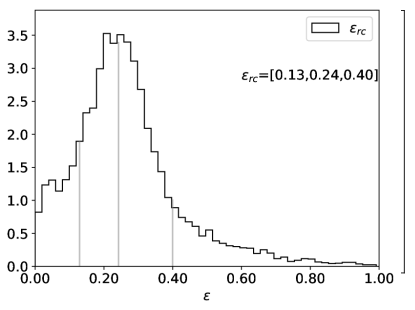
(f)

Figure 21: Ellipticity distributions of the biaxially symmetric models. The numbers shown in brackets represent the 16th percentile, the mode, and the 84th percentile (also shown by means of vertical grey lines).

Table 20: Covariance matrix of the luminosity segregated EFF model.

	$\alpha_{c}\ \ [^{\circ}]$	$\delta_{c}\ \ [^{\circ}]$	$\phi$ [radians]	$r_{ca}$ [pc]	$r_{cb}$ [pc]	$\gamma$	$\kappa$ [pc$\cdot\rm{mag}^{-1}$]
$\alpha_{c}\ \ [^{\circ}]$	0.007	-0.001	-0.000	0.001	-0.001	-0.000	-0.000
$\delta_{c}\ \ [^{\circ}]$	-0.001	0.006	0.002	0.001	0.002	0.001	0.001
$\phi$ [radians]	-0.000	0.002	0.085	0.009	0.002	0.005	0.001
$r_{ca}$ [pc]	0.001	0.001	0.009	0.151	0.078	0.060	0.008
$r_{cb}$ [pc]	-0.001	0.002	0.002	0.078	0.126	0.061	0.012
$\gamma$	-0.000	0.001	0.005	0.060	0.061	0.048	0.004
$\kappa$ [pc$\cdot\rm{mag}^{-1}$]	-0.000	0.001	0.001	0.008	0.012	0.004	0.006

Table 21: Covariance matrix of the luminosity segregated GDP model.

	$\alpha_{c}\ \ [^{\circ}]$	$\delta_{c}\ \ [^{\circ}]$	$\phi$ [radians]	$r_{ca}$ [pc]	$r_{cb}$ [pc]	$\alpha$	$\beta$	$\gamma$	$\kappa$ [pc$\cdot\rm{mag}^{-1}$]
$\alpha_{c}\ \ [^{\circ}]$	0.010	-0.001	0.000	-0.000	-0.003	-0.001	-0.003	0.001	-0.001
$\delta_{c}\ \ [^{\circ}]$	-0.001	0.008	0.002	0.003	0.004	0.000	0.004	-0.001	0.001
$\phi$ [radians]	0.000	0.002	0.321	0.102	0.064	0.010	0.071	-0.012	0.014
$r_{ca}$ [pc]	-0.000	0.003	0.102	1.122	0.789	0.092	0.506	-0.003	0.061
$r_{cb}$ [pc]	-0.003	0.004	0.064	0.789	0.828	0.072	0.472	-0.011	0.069
$\alpha$	-0.001	0.000	0.010	0.092	0.072	0.051	0.068	-0.019	0.004
$\beta$	-0.003	0.004	0.071	0.506	0.472	0.068	0.354	-0.040	0.040
$\gamma$	0.001	-0.001	-0.012	-0.003	-0.011	-0.019	-0.040	0.031	-0.003
$\kappa$ [pc$\cdot\rm{mag}^{-1}$]	-0.001	0.001	0.014	0.061	0.069	0.004	0.040	-0.003	0.016

Table 22: Covariance matrix of the luminosity segregated GKing model.

	$\alpha_{c}\ \ [^{\circ}]$	$\delta_{c}\ \ [^{\circ}]$	$\phi$ [radians]	$r_{ca}$ [pc]	$r_{ta}$ [pc]	$r_{cb}$ [pc]	$r_{tb}$ [pc]	$\alpha$	$\beta$	$\kappa$ [pc$\cdot\rm{mag}^{-1}$]
$\alpha_{c}\ \ [^{\circ}]$	0.015	-0.001	-0.003	0.002	-0.054	-0.007	-0.032	0.003	-0.003	-0.002
$\delta_{c}\ \ [^{\circ}]$	-0.001	0.012	0.006	0.004	0.076	0.017	0.033	-0.000	0.007	0.003
$\phi$ [radians]	-0.003	0.006	0.306	0.060	0.406	0.186	0.138	-0.017	0.067	0.027
$r_{ca}$ [pc]	0.002	0.004	0.060	4.645	1.703	2.322	1.919	0.388	0.563	0.167
$r_{ta}$ [pc]	-0.054	0.076	0.406	1.703	85.273	4.036	19.497	-0.637	2.217	0.511
$r_{cb}$ [pc]	-0.007	0.017	0.186	2.322	4.036	2.409	2.465	0.135	0.632	0.226
$r_{tb}$ [pc]	-0.032	0.033	0.138	1.919	19.497	2.465	17.347	-0.149	1.308	0.292
$\alpha$	0.003	-0.000	-0.017	0.388	-0.637	0.135	-0.149	0.342	0.023	-0.003
$\beta$	-0.003	0.007	0.067	0.563	2.217	0.632	1.308	0.023	0.232	0.067
$\kappa$ [pc$\cdot\rm{mag}^{-1}$]	-0.002	0.003	0.027	0.167	0.511	0.226	0.292	-0.003	0.067	0.037

Table 23: Covariance matrix of the luminosity segregated King model.

	$\alpha_{c}\ \ [^{\circ}]$	$\delta_{c}\ \ [^{\circ}]$	$\phi$ [radians]	$r_{ca}$ [pc]	$r_{ta}$ [pc]	$r_{cb}$ [pc]	$r_{tb}$ [pc]	$\kappa$ [pc$\cdot\rm{mag}^{-1}$]
$\alpha_{c}\ \ [^{\circ}]$	0.018	-0.001	-0.003	0.015	-0.105	0.002	-0.019	-0.000
$\delta_{c}\ \ [^{\circ}]$	-0.001	0.014	0.004	-0.009	0.123	-0.001	0.010	0.000
$\phi$ [radians]	-0.003	0.004	0.328	-0.118	1.317	-0.005	-0.064	0.004
$r_{ca}$ [pc]	0.015	-0.009	-0.118	1.547	-5.348	0.110	-1.293	0.002
$r_{ta}$ [pc]	-0.105	0.123	1.317	-5.348	220.118	-1.423	16.847	-0.041
$r_{cb}$ [pc]	0.002	-0.001	-0.005	0.110	-1.423	0.192	-1.046	0.014
$r_{tb}$ [pc]	-0.019	0.010	-0.064	-1.293	16.847	-1.046	32.386	-0.069
$\kappa$ [pc$\cdot\rm{mag}^{-1}$]	-0.000	0.000	0.004	0.002	-0.041	0.014	-0.069	0.004

Table 24: Covariance matrix of the luminosity segregated OGKing model.

	$\alpha_{c}\ \ [^{\circ}]$	$\delta_{c}\ \ [^{\circ}]$	$\phi$ [radians]	$r_{ca}$ [pc]	$r_{ta}$ [pc]	$r_{cb}$ [pc]	$r_{tb}$ [pc]	$\kappa$ [pc$\cdot\rm{mag}^{-1}$]
$\alpha_{c}\ \ [^{\circ}]$	0.009	-0.000	-0.002	0.002	-0.010	-0.000	-0.005	-0.001
$\delta_{c}\ \ [^{\circ}]$	-0.000	0.006	0.002	-0.002	0.013	0.002	-0.005	0.001
$\phi$ [radians]	-0.002	0.002	0.176	-0.019	0.137	0.008	-0.104	0.008
$r_{ca}$ [pc]	0.002	-0.002	-0.019	0.175	-0.381	0.025	-0.080	-0.002
$r_{ta}$ [pc]	-0.010	0.013	0.137	-0.381	10.973	-0.093	-0.386	0.009
$r_{cb}$ [pc]	-0.000	0.002	0.008	0.025	-0.093	0.070	-0.186	0.008
$r_{tb}$ [pc]	-0.005	-0.005	-0.104	-0.080	-0.386	-0.186	2.807	-0.023
$\kappa$ [pc$\cdot\rm{mag}^{-1}$]	-0.001	0.001	0.008	-0.002	0.009	0.008	-0.023	0.005

Table 25: Covariance matrix of the luminosity segregated RGDP model.

	$\alpha_{c}\ \ [^{\circ}]$	$\delta_{c}\ \ [^{\circ}]$	$\phi$ [radians]	$r_{ca}$ [pc]	$r_{cb}$ [pc]	$\alpha$	$\beta$	$\kappa$ [pc$\cdot\rm{mag}^{-1}$]
$\alpha_{c}\ \ [^{\circ}]$	0.010	-0.000	-0.000	0.002	0.001	-0.000	0.001	-0.001
$\delta_{c}\ \ [^{\circ}]$	-0.000	0.008	0.003	0.006	0.009	0.001	0.006	0.002
$\phi$ [radians]	-0.000	0.003	0.237	0.078	0.056	0.003	0.046	0.012
$r_{ca}$ [pc]	0.002	0.006	0.078	1.481	1.074	0.125	0.667	0.081
$r_{cb}$ [pc]	0.001	0.009	0.056	1.074	1.078	0.090	0.609	0.088
$\alpha$	-0.000	0.001	0.003	0.125	0.090	0.050	0.062	0.005
$\beta$	0.001	0.006	0.046	0.667	0.609	0.062	0.390	0.047
$\kappa$ [pc$\cdot\rm{mag}^{-1}$]	-0.001	0.002	0.012	0.081	0.088	0.005	0.047	0.016

(a)

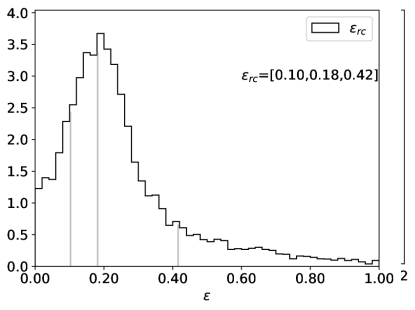
(b)

(c)

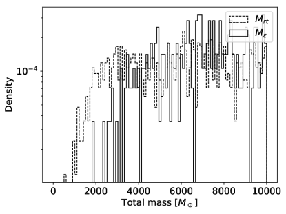
(d)

(e)

(f)

Figure 22: Inferred density of the luminosity segregated models. The data are binned in three bins of the J band: $J<12$, $12\lesssim J\lesssim 15$, and $15<J$ (with colours green, cyan and magenta, respectively). The MAP is shown by means of three coloured solid lines, the colours correspond to those of the $J$ band bins. In these MAPs, the core radius is increased accordingly to Eq. 13 using the mean value of the J band in each bin. Also shown are 100 samples from the posterior distribution (grey lines).

Figure 23: Projections of the posterior distribution for the luminosity segregated EFF model.

Figure 24: Projections of the posterior distribution for the luminosity segregated GDP model.

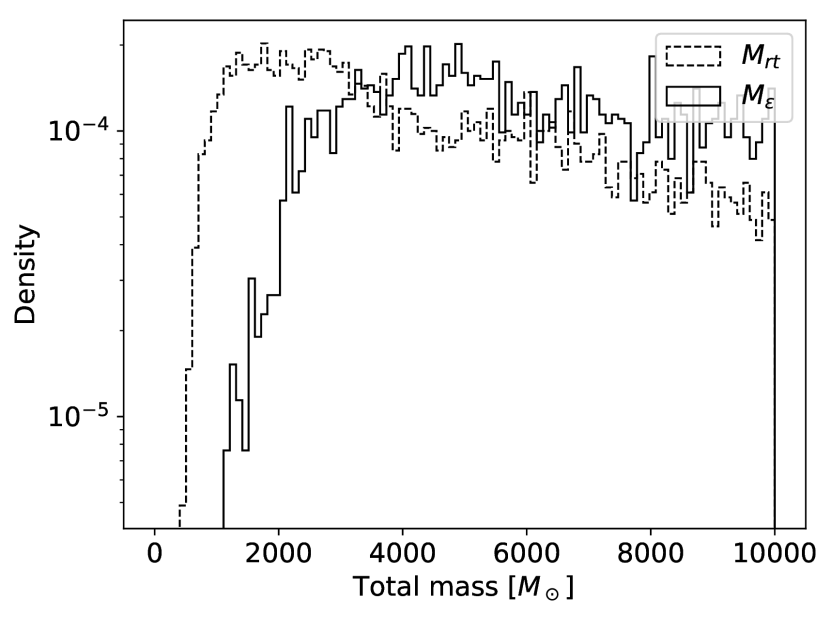
Figure 25: Projections of the posterior distribution for the luminosity segregated GKing model.

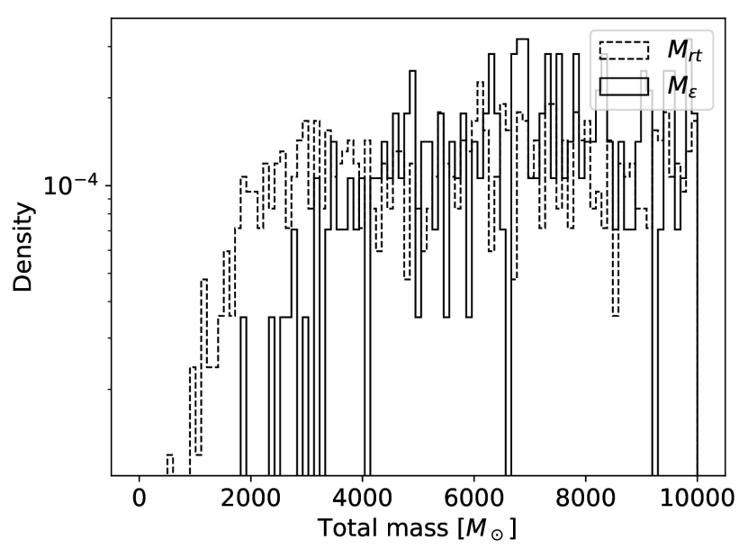
Figure 26: Projections of the posterior distribution for the luminosity segregated King’s model.

Figure 27: Projections of the posterior distribution for the luminosity segregated OGKing model.

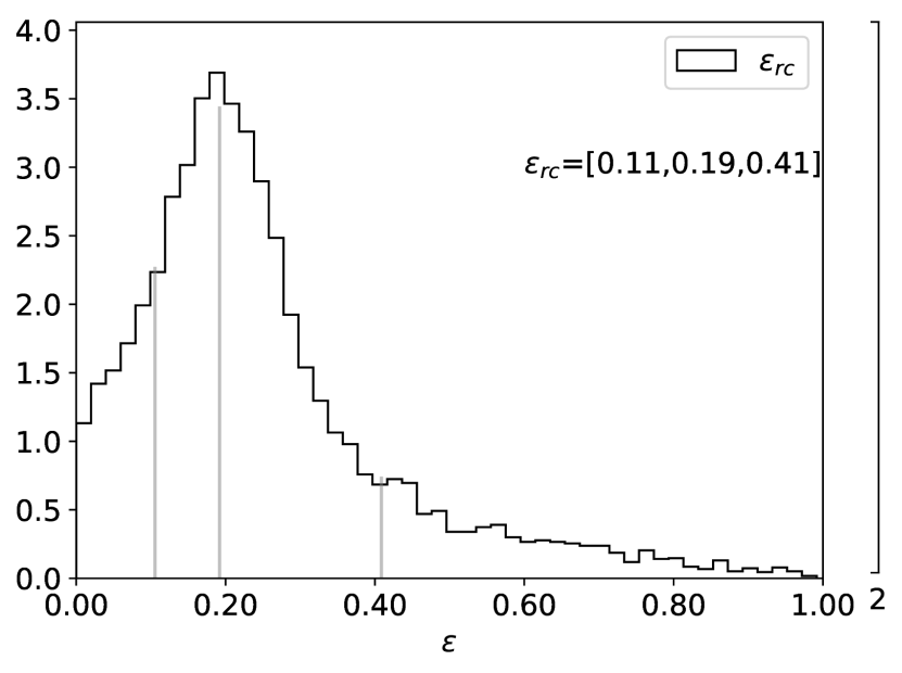
Figure 28: Projections of the posterior distribution for the luminosity segregated RGDP model.

(a)

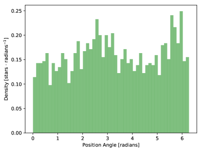
(b)

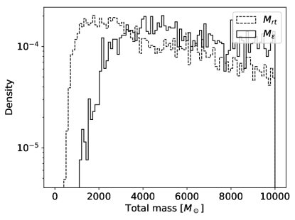
(c)

(d)

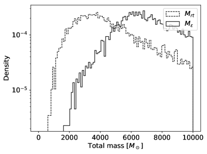
(e)

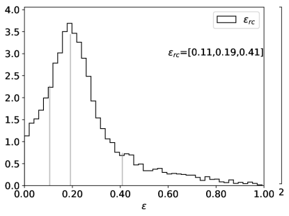
(f)

Figure 29: Ellipticity distributions of the luminosity segregated models. The numbers shown in brackets represent the 16th percentile, the mode, and the 84th percentile (also shown by means of vertical grey lines).

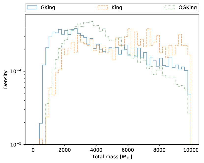
Figure 30: Distribution of the total mass of the cluster derived from each radially symmetric model of the King’s family.

Figure 31: Distribution of the total mass of the cluster derived from each biaxially symmetric model of the King’s family.