Valid Inference Corrected for Outlier Removal

Abstract

Ordinary least square (OLS) estimation of a linear regression model is well-known to be highly sensitive to outliers. It is common practice to (1) identify and remove outliers by looking at the data and (2) to fit OLS and form confidence intervals and $p$-values on the remaining data as if this were the original data collected. This standard “detect-and-forget” approach has been shown to be problematic, and in this paper we highlight the fact that it can lead to invalid inference and show how recently developed tools in selective inference can be used to properly account for outlier detection and removal. Our inferential procedures apply to a general class of outlier removal procedures that includes several of the most commonly used approaches. We conduct simulations to corroborate the theoretical results, and we apply our method to three real data sets to illustrate how our inferential results can differ from the traditional detect-and-forget strategy. A companion R package, outference, implements these new procedures with an interface that matches the functions commonly used for inference with lm in R.

Keywords: confidence intervals, linear regression, outlier, $p$-value, selective inference

1 Introduction

Linear regression is routinely used in just about every field of science. In introductory statistics courses, students are shown cautionary examples of how even a single outlier can wreak havoc in ordinary least squares (OLS). Outliers can arise for a variety of reasons, including recording errors and the occurrence of rare phenomena, and they often go unnoticed without careful inspection (see, e.g., Belsley et al., 2005). Given this reality, one simple strategy adopted by practitioners is a two-step procedure which we will refer to as detect-and-forget:

1. detect and then remove outliers;

2. fit OLS and perform inference on the remaining data as if this were the original data set.

While this simple approach is extremely common, there are two major problems (Welsh and Ronchetti, 2002). First, accurate detection of outliers can be challenging: In the presence of multiple outliers, classical influence measures, such as OLS residuals, Cook’s distance (Cook, 1977), and DFFITS (Welsch and Kuh, 1977), can be misleading, leading potentially to missed outliers and falsely detected outliers (see, e.g., Hadi and Simonoff, 1993, for more on “masking” and “swamping”). This first problem has received considerable attention, leading to the development of robust regression methods, in which one uses methods that are less sensitive to outliers (see, e.g., Maronna et al., 2006). A foundational method in this category is Huber’s M-estimator (Huber and Ronchetti, 1981), where one minimizes Huber’s loss function:

$$\underset{\beta\in\mathbb{R}^{p}}{\min}\ \frac{1}{n}\sum_{i=1}^{n}\rho(y_{i}-X_{i,\operatorname*{\scalerel*{\cdot}{\bigodot}}}\beta,\lambda)\qquad\text{ where }\qquad\rho(r,\lambda)=\begin{cases}\frac{1}{2}r^{2}&\text{ if }|r|\leq\lambda\\ \lambda|r|-\frac{1}{2}\lambda^{2}&\text{ if }|r|>\lambda,\end{cases}$$ (1)

where $X_{i,\operatorname*{\scalerel*{\cdot}{\bigodot}}}$ is $i$-th row of the design matrix. The “vanilla” Huber’s estimator has been shown to be insufficiently robust (Rousseeuw, 1984; Zaman et al., 2001), but state-of-the-art robust methods do exist, such as MM-estimation (Yohai, 1987).

This first problem with detect-and-forget has received much attention; the focus of this paper, however, is on a second problem. In the second step of the detect-and-forget approach, in which one performs downstream statistical inference based on the refitted OLS estimator, we show that the confidence intervals and hypothesis tests have incorrect operating characteristics. This second issue is orthogonal to the first: whether or not one is able to accurately identify outliers, if one chooses to search for and remove outliers, one must account for this step when doing subsequent inference. We emphasize that our solution to this second problem does not address the first problem of accurate outlier detection. Given the widespread continued use of classical outlier detection methods, we develop a practical fix to this second problem, allowing for valid inference after using the classical outlier detection methods (including OLS residuals, Cook’s distance and DFFITS) or after using Huber’s estimator.

The inferential problem with detect-and-forget stems from its use of the same data twice. While the term “outlier removal” might lead one to think of Step 1 as a clear-cut, essentially deterministic step, in fact Step 1 should instead be thought of as “potential outlier removal,” an imperfect process in which one has some probability of removing non-outliers, a process that can alter the distribution of the data. The act of searching for and removing potential outliers must be considered as part of the data-fitting procedure and thus must be considered in Step 2 when inference is being performed. Similar concerns over “double dipping” are well-known in prediction problems, in which sample splitting (into training and testing sets) is a common remedy. However, such a strategy does not translate in an obvious way to the outlier problem: suppose one splits the observations into two sets, searching for and removing potential outliers on the first set and then performing inference on the second set of observations. In such a case, one is of course left vulnerable to outliers in the second set throwing off the inference stage.

The idea of properly accounting for a previous look at the data is known as selective inference (Yekutieli, 2012; Taylor and Tibshirani, 2015). Much recent work is focused specifically on accounting for selection of a set of variables before performing inference (Fithian et al., 2014; Loftus and Taylor, 2015; Lee et al., 2016; Panigrahi et al., 2016). In our case, the selection is of observations rather than variables, but we show that the machinery of Loftus and Taylor (2015); Lee et al. (2016), namely conditioning on a stochastic selection event, can be naturally adapted to our context.

In fact, illustration of the problem with detect-and-forget has appeared in some literature. Berenguer-Rico and Wilms (2018) showed how the White test for heteroscedasticity can fail using the detect-and-forget approach under asymmetric errors; however, when the errors come from a symmetric distribution, they show how the theory of Berenguer-Rico and Nielsen (2017) can lead to the detect-and-forget approach being valid asymptotically and having good finite-sample performance.

We will now illustrate that even under symmetric errors, the detect-and-forget strategy can be problematic when performing inference for each covariate. As a toy example, consider the situation shown in Figure 1, in which there are 19 “normal” points (in black), and a single “outlier” point (in red) has been shifted upward by different magnitudes. For this illustration, we use a well-known approach for outlier detection called Cook’s distance (Cook, 1977):

$$D_{i}=\frac{\widehat{\varepsilon}_{i}^{2}}{p\widehat{\sigma}^{2}}\frac{h_{ii}}{(1-h_{ii})^{2}},$$ (2)

where $\widehat{\varepsilon}_{i}$ is the $i$-th residual from OLS on the entire data set, $\widehat{\sigma}^{2}:=\|\widehat{\varepsilon}\|_{2}^{2}/(n-p)$ is the scaled sum of squares, and $h_{ii}$ is the $i$-th diagonal entry of the hat matrix $X(X^{T}X)^{-1}X^{T}$. We declare the observation with the largest Cook’s distance to be the outlier (indicated in the figure by an open black box) and then refit the regression model with this point removed (black regression line). We then construct confidence intervals for the regression surface in two different ways: first, using the traditional detect-and-forget strategy, which ignores the outlier removal step, and second using corrected, a method we will introduce in this paper, which properly corrects for the removal. When the outlier is obvious (leftmost panel), our method makes no discernible correction. With such a pronounced separation between the outlier and non-outliers, Step 1 is unlikely to have removed a non-outlier, and thus the distribution of the data for inference is likely unaltered. However, when the outlier is less easily distinguished from the data, our corrected confidence intervals are noticeably different from the classical ones. In particular, the corrected intervals are pulled in the direction of the removed data point, thereby accounting for the possibility that the removed point may not in fact have been an outlier.

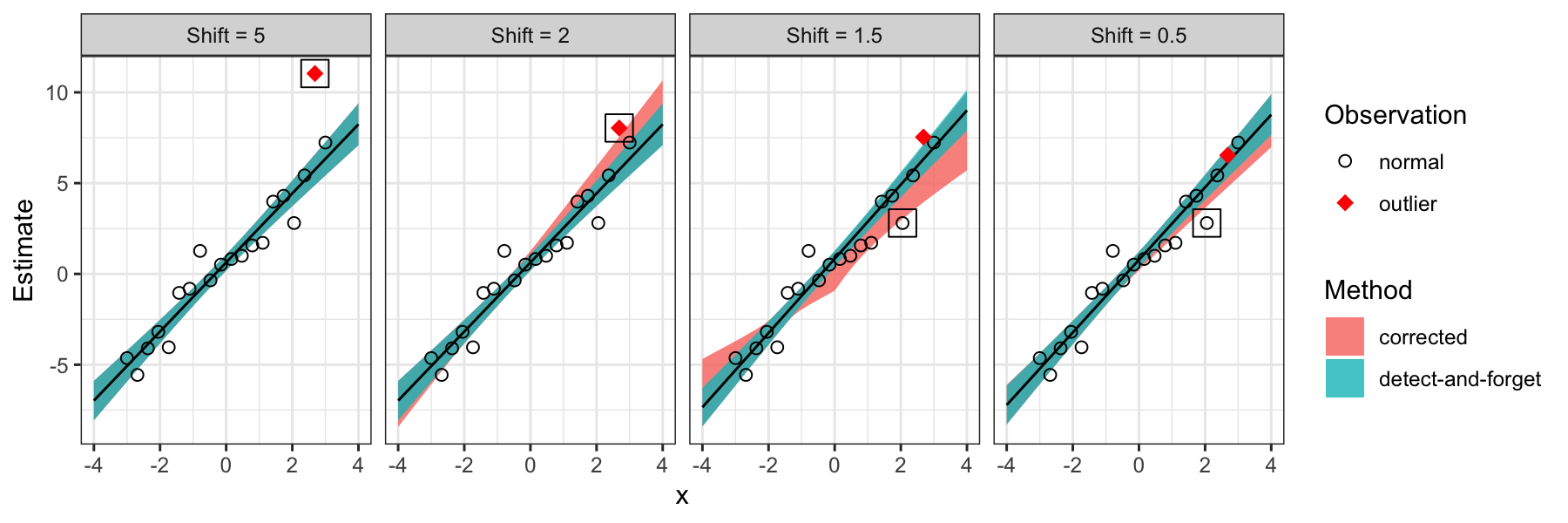
Figure 1: Confidence intervals for the regression surface. Normal data are in black while the only outlier is marked in red. The point with an open black box is the detected outlier which has the largest Cook’s distance. The black line is the regression line fitted using the data in which the detected outlier is removed.

While Figure 1 shows only a single realization of the two intervals in four different scenarios, Figure 2 shows the empirical coverage probability, averaged over 2000 realizations, of these two types of confidence intervals along the regression surface for the same four scenarios. We see that when the outlier signal is strong (leftmost panel), both detect-and-forget and corrected intervals achieve $95\%$ coverage, as desired. However, as the outlier signal decreases, the detect-and-forget intervals begin to break down, while our corrected intervals remain unaffected. Indeed, we will show in this paper how all sorts of inferential statements (confidence intervals for regression coefficients, coefficient $t$-tests, $F$-tests, etc.) can be thrown off using a detect-and-forget strategy but can be corrected with a proper accounting for the outlier detection and removal step.

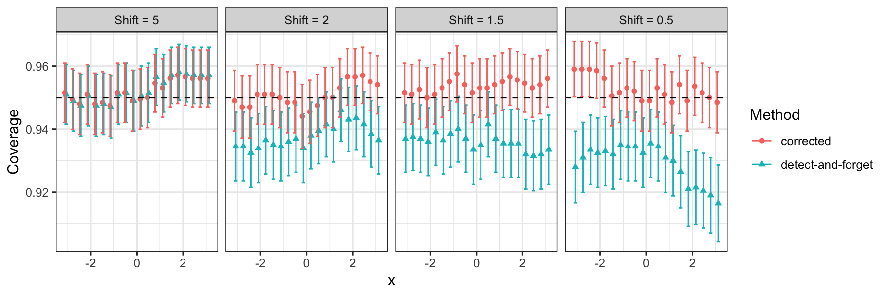
Figure 2: Empirical coverage probability along the regression surface (across $2000$ realizations). The dashed line represents $95\%$ coverage.

The machinery underlying our methodology is built on recent advances in selective inference (Fithian et al., 2014; Taylor and Tibshirani, 2015), specifically the framework introduced in Lee et al. (2016); Loftus and Taylor (2015), and it fits within the framework of inferactive data analysis introduced by Bi et al. (2017). We give a brief introduction to the philosophy of selective inference in the context of outlier detection and refer readers to Fithian et al. (2014) for more details.

We assume a standard regression setting, $(\mathbf{y},X)\in\mathbb{R}^{n}\times\mathbb{R}^{n\times p}$ with $\mathbf{y}\sim N(\boldsymbol{\mu},\sigma^{2}I_{n})$, where $\boldsymbol{\mu}_{i}=\mathbf{x}_{i}^{T}\boldsymbol{\beta}^{*}$ for $i\in M^{*}$ and $\mathbf{x}_{i}$ is the $i$-th row of $X$. Here $M^{*}$ is the set of non-outliers. If $M$ is the set of detected non-outliers, then the detect-and-forget strategy forms the OLS estimator on the subset of observations in $M$, $\hat{\boldsymbol{\beta}}^{M}=X_{M,\operatorname*{\scalerel*{\cdot}{\bigodot}}}^{+}\mathbf{y}_{M}$ (where $\mathbf{y}_{M}$ and $X_{M,\operatorname*{\scalerel*{\cdot}{\bigodot}}}$ are formed by taking rows indexed by $M$, and $X_{M,\operatorname*{\scalerel*{\cdot}{\bigodot}}}^{+}$ is the Moore-Penrose pseudoinverse of $X_{M,\operatorname*{\scalerel*{\cdot}{\bigodot}}}$), and then proceeds with inference assuming that $\hat{\boldsymbol{\beta}}^{M}\sim N(\boldsymbol{\beta}^{*},\sigma^{2}[X_{M,\operatorname*{\scalerel*{\cdot}{\bigodot}}}^{T}X_{M,\operatorname*{\scalerel*{\cdot}{\bigodot}}}]^{-1}).$

However, the above assumes that $M$ is non-random (or at least independent of $\mathbf{y}$) and that $M\subseteq M^{*}$, i.e. all true outliers have been successfully removed. However, in practice the set of declared non-outliers is in fact a function of the data, $\widehat{M}(\mathbf{y},X)$, and thus to perform inference would in principle require an understanding of the distribution of the much more complicated random variable $\hat{\boldsymbol{\beta}}^{\widehat{M}(\mathbf{y},X)}=X_{\widehat{M}(\mathbf{y},X),\operatorname*{\scalerel*{\cdot}{\bigodot}}}^{+}\mathbf{y}_{\widehat{M}(\mathbf{y},X)}.$

For general outlier removal procedures $\widehat{M}(\mathbf{y},X)$, such as “make plots and inspect by eye”, the above distribution may be completely unobtainable. However, in this paper we define a class of outlier removal procedures for which the conditional distribution $\hat{\boldsymbol{\beta}}^{\widehat{M}(\mathbf{y},X)}~{}|~{}\widehat{M}(\mathbf{y},X)$ can be precisely characterized. Access to this conditional distribution will allow us to construct confidence intervals and $p$-values that are valid conditional on the set of outliers selected.

For example, we will produce a procedure for forming outlier-removal-aware confidence intervals $C_{j}^{M}(\mathbf{y},X)$ such that $\mathbb{P}(\boldsymbol{\beta}^{*}_{j}\in C^{M}_{j}(\mathbf{y},X)\ |\ \widehat{M}(\mathbf{y},X)=M)\geq 1-\alpha$ for all subsets $M$ that do not include a true outlier.

If one could be certain that $\widehat{M}(\mathbf{y},X)\subseteq M^{*}$ (i.e., the procedure is adjusted to be sufficiently conservative and outliers are known to be sufficiently large), then such conditional coverage statements can be translated into a marginal (i.e., traditional) coverage statement: $\mathbb{P}(\boldsymbol{\beta}^{*}_{j}\in C^{\widehat{M}(\mathbf{y},X)}_{j}(\mathbf{y},X))\geq 1-\alpha.$

However, in practice we do not know if all true outliers have been successfully removed. If $\widehat{M}(\mathbf{y},X)\not\subseteq M^{*}$, then OLS is no longer guaranteed to produce an unbiased estimate of $\boldsymbol{\beta}^{*}$. OLS performed on the observations in $M$ instead estimates a parameter $\boldsymbol{\beta}^{M}$, which depends on both $\boldsymbol{\beta}^{*}$ and on $\mu_{M\setminus M^{*}}$, the mean of the true outliers that were not detected:

$$\boldsymbol{\beta}^{M}:=\underset{\boldsymbol{\beta}\in\mathbb{R}^{p}}{\arg\min}\ \mathbb{E}[\|\mathbf{y}_{M}-X_{M,\operatorname*{\scalerel*{\cdot}{\bigodot}}}\boldsymbol{\beta}\|_{2}^{2}]=X_{M,\operatorname*{\scalerel*{\cdot}{\bigodot}}}^{+}\boldsymbol{\mu}_{M}.$$ (3)

The goal of this paper is not to improve the performance of outlier removal procedures—certainly there is already extensive work in the literature on outlier removal. Rather, our goal is to provide valid inferential statements for someone who has chosen to use a particular outlier removal procedure, $\widehat{M}(\mathbf{y},X)$. Thus, to stay within the scope of this problem, we will simply acknowledge that if a procedure $\widehat{M}(\mathbf{y},X)$ is prone to failing to identify outliers, then one cannot hope to estimate $\boldsymbol{\beta}^{*}$ but must instead focus on estimating and performing inference for $\boldsymbol{\beta}^{\widehat{M}(\mathbf{y},X)}$, which reflects more accurately than $\boldsymbol{\beta}^{*}$ the relationship between $X$ and $\mathbf{y}$ in the data that is provided to us by $\widehat{M}(\mathbf{y},X)$. For example, we will provide intervals with guaranteed coverage of $\boldsymbol{\beta}^{\widehat{M}(\mathbf{y},X)}$: $\mathbb{P}(\boldsymbol{\beta}^{\widehat{M}(\mathbf{y},X)}_{j}\in C^{\widehat{M}(\mathbf{y},X)}_{j}(\mathbf{y},X))\geq 1-\alpha.$ We will likewise provide all the standard confidence intervals and hypothesis tests for regression but focused on $\boldsymbol{\beta}^{\widehat{M}(\mathbf{y},X)}$ in place of $\boldsymbol{\beta}^{*}$.

This discussion emphasizes the inherently different effect of false positives (i.e., removing points that are not true outliers) versus false negatives (i.e., failing to remove points that are true outliers). When all true outliers are removed, $\boldsymbol{\beta}^{\widehat{M}}=\boldsymbol{\beta}^{*}$, and our machinery gives corrected inferential statements that account for the outlier removal step (including accounting for any false positives). By contrast, when true outliers remain, $\boldsymbol{\beta}^{\widehat{M}}\neq\boldsymbol{\beta}^{*}$, both detect-and-forget and our procedure give inferential statements about $\boldsymbol{\beta}^{\widehat{M}}$ rather than $\boldsymbol{\beta}^{*}$; however, in the case of our method, these statements are at least valid.

The rest of the paper is organized as follows: in Section 2 we formulate the problem more precisely and describe the class of outlier detection procedures over which our framework applies; Section 3 describes our methodology for forming confidence intervals and extracting $p$-values that are properly corrected for outlier removal; Section 4 provides empirical comparisons of the naive detect-and-forget strategy and our method, both through comprehensive simulations and a re-analysis of three real data sets; Section 5 gives a discussion and possible next steps. A companion R package, outference, is available at https://github.com/shuxiaoc/outference. For brevity, we collect proofs of most theoretical results, some additional simulation results and the implementation details in the online supplementary material.

We conclude this section by introducing some notation that will be used throughout this paper. For $n\in\mathbb{N}$, we let $[n]:=\{1,2,\ldots,n\}$. For a matrix $X$, we let $\mathscr{C}(X)$ be its column space and $\text{tr}(X)$ be its trace. We let $X_{I,J}$ be the submatrix formed by rows and columns indexed by $I$ and $J$, respectively, and we let $X_{I,\operatorname*{\scalerel*{\cdot}{\bigodot}}}$ be the submatrix formed by rows indexed by $I$. We let $P_{X}$ be the projection matrix onto $\mathscr{C}(X)$ and $P_{X}^{\perp}:=I-P_{X}$. For a submatrix $X_{I,J}$, we write $P_{I,J}:=P_{X_{I,J}}$ when there is no ambiguity. We use $\mathrel{\text{\scalebox{1.07}{$\perp\mkern-10.0mu\perp$}}}$ to denote statistical independence.

2 Problem Formulation

2.1 The General Setup

We elaborate on the framework described in the previous section, introducing some additional notation. We assume $\mathbf{y}=\boldsymbol{\mu}+\boldsymbol{\varepsilon}$, where $\mathbf{y}\in\mathbb{R}^{n},\boldsymbol{\varepsilon}\sim N(\mathbf{0},\sigma^{2}I_{n})$ and consider the mean-shift model,

$$\boldsymbol{\mu}=X\boldsymbol{\beta}^{*}+\mathbf{u}^{*},$$ (4)

where $\boldsymbol{\beta}^{*}\in\mathbb{R}^{p}$, and $X$ is a non-random matrix of predictors. The set $M^{*}=[n]\setminus\text{supp}(\mathbf{u}^{*})$ is the index set of true non-outliers; equivalently, $M^{*c}$ is the index set of true outliers. By definition of $M^{*}$, $\mathbf{u}^{*}_{M^{*}}=\mathbf{0}$ and $\mathbf{u}^{*}_{i}\neq 0$ for $i\in M^{*c}$. This setup assumes that all outliers considered are “vertical” in the sense that they only contaminate the model in the $y$-direction. We denote a data-dependent outlier removal procedure, $\widehat{M}:\mathbb{R}^{n}\to 2^{[n]}$, as a function mapping the data $\mathbf{y}$ to the index set of detected non-outliers (for notational ease, we suppress the dependence of $\widehat{M}$ on $X$ since $X$ is treated as non-random). We will assume throughout that $X_{\widehat{M}(\mathbf{y}),\operatorname*{\scalerel*{\cdot}{\bigodot}}}$ has linearly independent columns.

For a fixed subset of the observations $M\subseteq[n]$, the parameter $X\boldsymbol{\beta}^{M}$ where $\boldsymbol{\beta}^{M}$ is defined in (3) represents the best linear approximation of $\boldsymbol{\mu}_{M}$ using the $p$ predictors in $X_{M,\operatorname*{\scalerel*{\cdot}{\bigodot}}}$. In what follows, we will provide hypothesis tests and confidence intervals for $\boldsymbol{\beta}^{M}$ conditional on the event $\{\widehat{M}(\mathbf{y})=M\}$.

Combining (3) and (4) with the assumption that $X_{M,\operatorname*{\scalerel*{\cdot}{\bigodot}}}$ has linearly independent columns, we have $\boldsymbol{\beta}^{M}=X_{M,\operatorname*{\scalerel*{\cdot}{\bigodot}}}^{+}(X_{M,\operatorname*{\scalerel*{\cdot}{\bigodot}}}\boldsymbol{\beta}^{*}+\mathbf{u}^{*}_{M})=\boldsymbol{\beta}^{*}+X_{M,\operatorname*{\scalerel*{\cdot}{\bigodot}}}^{+}\mathbf{u}^{*}_{M}$. Since $\mathbf{u}^{*}_{M^{*}}=0$, it follows that $\boldsymbol{\beta}^{M}=\boldsymbol{\beta}^{*}$ when $M\subseteq M^{*}$. This result makes it clear that if one wishes to make statements about $\beta^{*}$, then one must ensure that the procedure $\widehat{M}$ is screening out all outliers.

Our focus will be on performing inference on $\boldsymbol{\beta}^{M}$ conditional on the event $\{\widehat{M}(\mathbf{y})=M\}$. Importantly, such inferential procedures in fact provide asymptotically valid inferences for $\boldsymbol{\beta}^{*}$ as long as one’s outlier removal procedure asympotically detects all outliers. For example, the next proposition establishes that confidence intervals providing conditional coverage of $\boldsymbol{\beta}^{M}_{j}$ given $\{\widehat{M}(\mathbf{y})=M\}$ do in fact achieve traditional (i.e., unconditional) coverage of $\boldsymbol{\beta}^{*}_{j}$ asymptotically if one is using an outlier detection procedure that is guaranteed to screen out all outliers as $n\to\infty$.

Proposition 2.1.

For $\mathbf{y}$ generated through the mean-shift model (4), consider intervals $C_{j}^{\widehat{M}}$, satisfying $\mathbb{P}(\boldsymbol{\beta}^{\widehat{M}}_{j}\in C_{j}^{\widehat{M}}\ |\ \widehat{M}=M)=1-\alpha$. If the outlier detection procedure $\widehat{M}$ satisfies $\mathbb{P}(\widehat{M}\subseteq M^{*})\to 1$ as $n\to\infty$, then we have $\mathbb{P}(\boldsymbol{\beta}^{*}_{j}\in C_{j}^{\widehat{M}})\to 1-\alpha$.

This proposition is based on two simple observations: first, that conditional coverage of $\boldsymbol{\beta}^{\widehat{M}}$ implies unconditional coverage of $\boldsymbol{\beta}^{\widehat{M}}$; second, that $\widehat{M}\subseteq M^{*}$ implies that $\boldsymbol{\beta}^{\widehat{M}}=\boldsymbol{\beta}^{*}$.

Such a screening property is reasonable to demand of an outlier detection procedure, and related results exist in the literature (Zhao et al., 2013). For example, consider using Cook’s distance (2) to detect outliers:

$$\widehat{M}(\mathbf{y})=\{i:D_{i}<\lambda/n\},$$ (5)

where $\lambda$ is a prespecified cutoff. In Section 2 of the supplementary material, we provide conditions (based on a result of Zhao et al. 2013) under which $\mathbb{P}(\widehat{M}=M^{*})\to 1$ for an appropriate choice of $\lambda$. While $\lambda=0$ would trivially satisfy the screening property, we of course need a procedure that leaves sufficient observations for estimation and inference.

While the mean-shift model model is common in the outlier detection literature, it is by no means the only reasonable one (see, e.g., Huber 1965; Thompson 1985; Huber 1992). We choose to focus on the mean-shift model because it provides a simple yet practical working definition of an “outlier”, and it is relatively easy to prove the effectiveness of the outlier detection procedure considered in this paper under this model (e.g., Proposition S.1 in the supplementary material). However, our main results are, indeed, independent of the choice of specific outlier model.

2.2 Quadratic Outlier Detection Procedures

In this section we define a general class of outlier detection procedures for which our methodology will apply. We then show that this class includes several of the most famous outlier detection procedures.

Definition 2.2.

We say an outlier detection procedure is quadratic if the event ${\{\widehat{M}(\mathbf{y})=M\}}=:\mathcal{E}_{M}$ is of the form $\mathfrak{X}(\{\mathcal{E}_{M,i}\}_{i\in I_{M}})$, where $\mathfrak{X}$ denotes a general set operator that maps a finite family of sets to a single set, $I_{M}$ is a finite index set, and $\mathcal{E}_{M,i}:=\{\mathbf{y}\in\mathbb{R}^{n}:\mathbf{y}^{T}Q_{M,i}\mathbf{y}+\mathbf{a}_{M,i}^{T}\mathbf{y}+b_{M,i}\geq 0\}$, for some $Q_{M,i}\in\mathbb{R}^{n\times n},\mathbf{a}_{M,i}\in\mathbb{R}^{n}$, and $b_{M,i}\in\mathbb{R}$.

Generally, $\mathfrak{X}$ should be thought of as taking finite unions, intersections, and complements. The above definition is a direct generalization of Definition 1.1 of Loftus and Taylor (2015), in which $\mathfrak{X}\equiv\bigcap$. We will see that many outlier detection procedures are quadratic in the sense of Definition 2.2. While most of the time the definition in Loftus and Taylor (2015) will apply, there are certain cases that require our generalization (see Section 3.2 of the supplementary material for a specific example). The next proposition shows that outlier detection using Cook’s distance is quadratic in the sense of Definition 2.2.

Proposition 2.3.

Outlier detection using Cook’s distance (5) is quadratic with

$$\mathcal{E}_{M} =\bigcap_{i\in[n]}\mathcal{E}_{M,i},$$ (6)

$$\mathcal{E}_{M,i} =\bigg{\{}\mathbf{y}\in\mathbb{R}^{n}:(-1)^{\mathbbm{1}\{i\in M^{c}\}}\mathbf{y}^{T}\bigg{(}\frac{\lambda p}{n}(1-h_{i})^{2}P_{X}^{\perp}-(n-p)h_{i}P_{X}^{\perp}\mathbf{e}_{i}\mathbf{e}_{i}^{T}P_{X}^{\perp}\bigg{)}\mathbf{y}>0\bigg{\}},$$ (7)

where $\mathbf{e}_{i}$ is $i$-th standard basis for $\mathbb{R}^{n}$ and $h_{i}=(P_{X})_{ii}$.

Proof.

We may write $D_{i}=\bigg{(}\mathbf{y}^{T}(P_{X}^{\perp}e_{i}e_{i}^{T}P_{X}^{\perp})\mathbf{y}\bigg{/}\mathbf{y}^{T}P_{X}^{\perp}\mathbf{y}\bigg{)}\cdot\bigg{(}(n-p)h_{i}\bigg{/}p(1-h_{i})^{2}\bigg{)}.$ Plugging this expression to $\widehat{M}=\{i:D_{i}<\lambda/n\}$ and $\widehat{M}^{c}=\{i:D_{i}\geq\lambda/n\}$ gives the desired result. ∎

As a second example, we consider Huber’s M-estimator (1). Though it is a robust regression method, (as observed in She and Owen 2011) its solution $\hat{\beta}_{\lambda}$ can be equivalently expressed as the following lasso program (Tibshirani, 1996) within the context of the mean-shift model:

$$(\hat{\boldsymbol{\beta}}_{\lambda},\hat{\mathbf{u}}_{\lambda})=\underset{\boldsymbol{\beta}\in\mathbb{R}^{p},\mathbf{u}\in\mathbb{R}^{n}}{\arg\min}\ \frac{1}{2n}\|\mathbf{y}-X\boldsymbol{\beta}-\mathbf{u}\|_{2}^{2}+\lambda\|\mathbf{u}\|_{1},$$ (8)

which the authors refer to as the soft-IPOD method. The $\ell_{1}$-penalty induces sparsity in $\hat{\mathbf{u}}_{\lambda}$, and one takes $\widehat{M}(\mathbf{y})=\{i:\hat{\mathbf{u}}_{\lambda,i}=0\}$ as the detected non-outliers. The outliers correspond to the elements whose residuals are in the quadratic (rather than linear) region of Huber’s loss function. In Section 3 of the supplementary material, this approach is shown to be a quadratic outlier detection procedure, which explains why our framework can accommodate this foundational robust regression method. The DFFITS outlier detection method (Welsch and Kuh, 1977) is described in Section 3 of the supplementary material, where it is shown to be quadratic. Extending our framework to state-of-the-art outlier detection methods (e.g., examining the residuals after MM-estimation) remains an open question.

3 Inference Corrected for Outlier Removal

In this section, we describe how the standard inferential tools of OLS can be corrected to account for outlier removal. The only requirement is that the outlier detection procedure be quadratic (as defined in the previous section). The inferential statements are made conditional on the event $\{\widehat{M}(\mathbf{y})=M\}$ and are about the parameter $\boldsymbol{\beta}^{M}$. As previously discussed, such statements translate to unconditional statements about $\beta^{*}$ when $\widehat{M}\subseteq M^{*}$, that is, when all true outliers are removed. Section 3.1 treats the case in which $\sigma$ is known. Section 3.2 provides procedures for the case when $\sigma$ is unknown.

3.1 Confidence Intervals and Hypothesis Tests When $\sigma$ Is Known

In this section, we suppose that $\sigma$ is known and provide confidence intervals and hypothesis tests. In the classical setting, inference is based on the normal and $\chi^{2}$ distributions and typically involves individual regression coefficients $\boldsymbol{\beta}^{M}_{j}$, the regression surface $\boldsymbol{x}_{0}^{T}\boldsymbol{\beta}^{M}$, or groups of regression coefficients $\boldsymbol{\beta}_{g}^{M}$. We begin by observing that both $\boldsymbol{\beta}^{M}_{j}$ and $\mathbf{x}_{0}^{T}\boldsymbol{\beta}^{M}$ are of the form $\boldsymbol{\nu}^{T}\boldsymbol{\mu}$ for some vector $\boldsymbol{\nu}$ that depends on $M$: $\boldsymbol{\beta}^{M}_{j}=\mathbf{e}_{j}^{T}X_{M,\operatorname*{\scalerel*{\cdot}{\bigodot}}}^{+}I_{M,\operatorname*{\scalerel*{\cdot}{\bigodot}}}\boldsymbol{\mu}$ and $\mathbf{x}_{0}^{T}\boldsymbol{\beta}^{M}=\mathbf{x}_{0}^{T}X_{M,\operatorname*{\scalerel*{\cdot}{\bigodot}}}^{+}I_{M,\operatorname*{\scalerel*{\cdot}{\bigodot}}}\boldsymbol{\mu}$. The next theorem gives a unified treatment of these two cases that will allow us to construct confidence intervals and $p$-values that properly account for outlier removal.

Theorem 3.1.

Assume the outlier detection procedure $\{\widehat{M}=M\}$ is quadratic as in Definition 2.2. Let $\boldsymbol{\nu}\in\mathbb{R}^{n}$ be a vector that may depend on $M$. Define

$$\mathcal{Z} :=\frac{\boldsymbol{\nu}^{T}\mathbf{y}}{\sigma\|\boldsymbol{\nu}\|_{2}},\ \ \ \mathbf{z}:=P_{\boldsymbol{\nu}}^{\perp}\mathbf{y}=\bigg{(}I-\frac{\boldsymbol{\nu}\boldsymbol{\nu}^{T}}{\|\boldsymbol{\nu}\|_{2}^{2}}\bigg{)}\mathbf{y}.$$

We have

$$\mathcal{Z}\ \bigg{|}\ \bigg{\{}\widehat{M}=M,\mathbf{z}\bigg{\}}\sim TN\bigg{(}\frac{\boldsymbol{\nu}^{T}\boldsymbol{\mu}}{\sigma\|\boldsymbol{\nu}\|_{2}},1;E_{M,\mathbf{z}}\bigg{)},$$ (9)

where the R.H.S is a $N(\frac{\boldsymbol{\nu}^{T}\boldsymbol{\mu}}{\sigma\|\boldsymbol{\nu}\|_{2}},1)$ random variable truncated to the set $E_{M,\mathbf{z}}$. The truncation set is defined in Section 4.2 of the supplementary material and can be computed by finding the roots of a finite set of quadratic polynomials. Thus, letting $F_{\xi,\gamma^{2}}^{E}$ be the CDF of a $TN(\xi,\gamma^{2};E)$ random variable, we have

$$1-F^{E_{M,\mathbf{z}}}_{\frac{\boldsymbol{\nu}^{T}\boldsymbol{\mu}}{\sigma\|\boldsymbol{\nu}\|_{2}},1}(\mathcal{Z})\ \bigg{|}\ \{\widehat{M}=M\}\sim\text{\emph{unif}}(0,1).$$ (10)

The classical analogue to the above theorem is the (much simpler!) statement that $\mathcal{Z}\sim N(\boldsymbol{\nu}^{T}\boldsymbol{\mu}/[\sigma\|\boldsymbol{\nu}\|_{2}],1)$.

This theorem is essentially a generalization of Lee et al. (2016, Theorem 5.2) and a special case of Loftus and Taylor (2015, Theorem 3.1); however, a key difference is that these works are focused on accounting for variable selection rather than outlier removal (which, in essence, is “observation selection”).

3.1.1 Corrected Confidence Intervals

We begin by applying Theorem 3.1 to get confidence intervals corrected for outlier removal.

Corollary 3.2.

Under the conditions and notation of Theorem 3.1, if we find $L$ and $U$ such that

$$L:F_{\frac{L}{\sigma\|\boldsymbol{\nu}\|_{2}},1}^{E_{M,\mathbf{z}}}(\mathcal{Z})=1-\frac{\alpha}{2},\ \ \ U:F_{\frac{U}{\sigma\|\boldsymbol{\nu}\|_{2}},1}^{E_{M,\mathbf{z}}}(\mathcal{Z})=\frac{\alpha}{2},$$ (11)

then $[L,U]$ is a valid $(1-\alpha)$ selective confidence interval for $\boldsymbol{\nu}^{T}\boldsymbol{\mu}$. That is,

$$\mathbb{P}(\boldsymbol{\nu}^{T}\boldsymbol{\mu}\in[L,U]\ |\ \widehat{M}=M)=1-\alpha.$$ (12)

This result encompasses the two most common types of confidence intervals arising in regression: intervals for the regression coefficients $\boldsymbol{\beta}^{M}_{j}$ and intervals for the regression surface $\mathbf{x}_{0}^{T}\boldsymbol{\beta}^{M}$.

Corollary 3.3.

We write $\boldsymbol{\beta}^{M}_{j}=\boldsymbol{\nu}_{\text{\emph{coef}},j}^{T}\boldsymbol{\mu}$ and $\mathbf{x}_{0}^{T}\boldsymbol{\beta}^{M}=\boldsymbol{\nu}_{\text{\emph{surf}}}^{T}\boldsymbol{\mu}$, where $\boldsymbol{\nu}_{\text{\emph{coef}},j}=(\mathbf{e}_{j}^{T}X_{M,\operatorname*{\scalerel*{\cdot}{\bigodot}}}^{+}I_{M,\operatorname*{\scalerel*{\cdot}{\bigodot}}})^{T}$ and $\boldsymbol{\nu}_{\text{\emph{surf}}}=(\mathbf{x}_{0}^{T}X_{M,\operatorname*{\scalerel*{\cdot}{\bigodot}}}^{+}I_{M,\operatorname*{\scalerel*{\cdot}{\bigodot}}})^{T}$. Then Theorem 3.1 and Corollary 3.2 apply.

A third type of interval common in regression is the prediction interval, intended to cover $\mathbf{x}_{0}^{T}\boldsymbol{\beta}^{M}+\boldsymbol{\varepsilon}_{0}$, where $\mathbf{x}_{0}\in\mathbb{R}^{p}$ is a new data point and $\boldsymbol{\varepsilon}_{0}\sim N(0,\sigma^{2})$ is independent of $\boldsymbol{\varepsilon}$. While $\boldsymbol{\nu}^{T}\mathbf{y}\ |\ \{\widehat{M}=M,\mathbf{z}\}$ is a truncated normal random variable, $\boldsymbol{\nu}^{T}\mathbf{y}+\boldsymbol{\varepsilon}_{0}\ |\ \{\widehat{M}=M,\mathbf{z}\}$ is not, so the strategy adopted in Theorem 3.1 does not directly apply to this case. Instead we employ a simple (but conservative) strategy.

Proposition 3.4.

Let $\varepsilon_{0}\sim N(0,\sigma^{2})$ be the noise independent of $\mathbf{y}$. For a given significance level $\alpha\in(0,1)$, let $\widetilde{\alpha}\in(0,\alpha)$. Given $\mathbf{x}_{0}\in\mathbb{R}^{p}$, let $[L_{\widetilde{\alpha}},U_{\widetilde{\alpha}}]$ be the $(1-\widetilde{\alpha})$ selective confidence intervals for $\mathbf{x}_{0}^{T}\boldsymbol{\beta}^{M}$ as defined in (11). Then we have

$$\mathbb{P}\bigg{(}L_{\widetilde{\alpha}}-\Phi^{-1}(1-\frac{\alpha-\widetilde{\alpha}}{2})\sigma\leq\mathbf{x}_{0}^{T}\boldsymbol{\beta}^{M}+\varepsilon_{0}\leq U_{\widetilde{\alpha}}+\Phi^{-1}(1-\frac{\alpha-\widetilde{\alpha}}{2})\sigma\ \bigg{|}\ \widehat{M}=M\bigg{)}\geq 1-\alpha,$$ (13)

where $\Phi$ is the CDF of a standard normal distribution.

In practice, we can optimize over $\widetilde{\alpha}$ so that the length of the interval is minimized.

3.1.2 Corrected Hypothesis Tests

Theorem 3.1 allows us to form selective hypothesis tests about the parameter $\boldsymbol{\nu}^{T}\boldsymbol{\mu}$ where $\boldsymbol{\nu}$ may depend on the selected index set of observations $M$.

Corollary 3.5.

Under the conditions and notation of Theorem 3.1, the quantity $1-F^{E_{M,\mathbf{z}}}_{0,1}(\mathcal{Z})$ gives a valid selective $p$-value for testing $H_{0}:\nu^{T}\mu=0$.

The most common application of the above would be for testing whether a specific regression coefficient is zero, conditional on $M$ being the selected set of non-outliers: $H_{0}(M,j):\boldsymbol{\beta}^{M}_{j}=0$ for $j\in[p]$.

As a generalization, we next focus on testing $H_{0}(M,g):\boldsymbol{\beta}^{M}_{g}=0$ for $g\subseteq[p]$. We begin with an alternative characterization of $H_{0}(M,g)$.

Proposition 3.6.

Set $\widetilde{X}_{M,g}=(I_{|M|}-P_{M,g^{c}})X_{M,g}$, where $P_{M,g^{c}}$ is the projection matrix onto $\mathscr{C}(X_{M,g^{c}})$. Let $\widetilde{P}_{M,g}$ be the projection matrix onto $\mathscr{C}(\widetilde{X}_{M,g})$. Then we have

$$\boldsymbol{\beta}^{M}_{g}=\mathbf{0}\Leftrightarrow\widetilde{X}_{M,g}^{+}\boldsymbol{\mu}_{M}=\mathbf{0}\Leftrightarrow\widetilde{P}_{M,g}\boldsymbol{\mu}_{M}=\mathbf{0}.$$ (14)

Further, define $\widecheck{P}_{M,g}:=\begin{pmatrix}\widetilde{P}_{M,g}&\mathbf{0}_{|M|\times(n-|M|)}\\ \mathbf{0}_{(n-|M|)\times|M|}&\mathbf{0}_{(n-|M|)\times(n-|M|)}\end{pmatrix}.$ Then $\widecheck{P}_{M,g}$ is an orthogonal projection matrix (it is symmetric and idempotent), and we have

$$\boldsymbol{\beta}^{M}_{g}=\mathbf{0}\Leftrightarrow\widecheck{P}_{M,g}\boldsymbol{\mu}=\mathbf{0}.$$ (15)

This proposition characterizes $H_{0}(M,g)$ as testing the projection of $\boldsymbol{\mu}$. In the non-selective case, testing $P\boldsymbol{\mu}=\mathbf{0}$ for some projection matrix $P$ can be done based on $\sigma^{-2}\mathbf{y}^{T}P\mathbf{y}\sim\chi^{2}_{\text{{tr}}(P)}$ under $P\boldsymbol{\mu}=\mathbf{0}$. We would expect that in the selective case, such tests can be done based on a truncated $\chi^{2}$ distribution.

Theorem 3.7.

Assume the outlier detection procedure $\{\widehat{M}=M\}$ is quadratic as in Definition 2.2. Define

$$\mathcal{X} :=\frac{\|\widecheck{P}_{M,g}\mathbf{y}\|_{2}}{\sigma},\ \ \ \mathbf{w}:=\frac{\widecheck{P}_{M,g}\mathbf{y}}{\|\widecheck{P}_{M,g}\mathbf{y}\|_{2}}=\frac{\widecheck{P}_{M,g}\mathbf{y}}{\sigma\mathcal{X}},\ \ \ \mathbf{z}:=\widecheck{P}_{M,g}^{\perp}\mathbf{y}.$$ (16)

Under $H_{0}(M,g):\boldsymbol{\beta}^{M}_{g}=0$, we have

$$\mathcal{X}^{2}\ \bigg{|}\ \{\widehat{M}=M,\mathbf{w},\mathbf{z}\}\sim T\chi^{2}_{\text{\emph{tr}}(\widecheck{P}_{M,g})}(E_{M,\mathbf{w},\mathbf{z}}),$$ (17)

where the R.H.S is a central $\chi^{2}$ random variable with $\text{df}=\text{\emph{tr}}(\widecheck{P}_{M,g})$ truncated to the set $E_{M,\mathbf{w},\mathbf{z}}$. The truncation set is defined in Section 4.5 of the supplementary material and can be computed by finding the roots of a finite set of quadratic polynomials. Further, letting $F_{df}^{E}$ be the CDF of a $T\chi^{2}_{df}(E)$ random variable, we have

$$1-F_{\text{\emph{tr}}(\widecheck{P}_{M,g})}^{E_{M,\mathbf{w},\mathbf{z}}}(\mathcal{X}^{2})\ \bigg{|}\ \{\widehat{M}=M\}\sim\text{\emph{unif}}(0,1),$$ (18)

which is a valid selective $p$-value for testing $H_{0}(M,g):(\boldsymbol{\beta}^{M})_{g}=0$.

This theorem is adapted from Loftus and Taylor (2015, Theorem 3.1) to the outlier detection context. In the special case where $g=j$ is a single index, direct computation can show that $\widecheck{P}_{M,j}=P_{\boldsymbol{\nu}_{\text{coef},j}}$, so that $\mathcal{X}^{2}=(\boldsymbol{\nu}^{T}_{\text{coef},j}\mathbf{y})^{2}/({\sigma\|\boldsymbol{\nu}_{\text{coef},j}\|_{2}})^{2},w=\text{sign}(\boldsymbol{\nu}_{\text{coef},j}^{T}\mathbf{y})\boldsymbol{\nu}_{\text{coef},j}$, and $\mathbf{z}=P_{\boldsymbol{\nu}_{\text{coef},j}}^{\perp}\mathbf{y}.$ Then this theorem nearly reduces to Theorem 3.1, except that in this theorem, we need to condition on the sign of $\boldsymbol{\nu}_{\text{coef},j}^{T}\mathbf{y}$.

3.2 Extension to $\boldsymbol{\sigma}$ Unknown Case

In this section, we extend results in Section 3.1.2 to the $\sigma$ unknown case. In the non-selective case, the hypothesis $H_{0}:\boldsymbol{\beta}^{*}_{g}=\mathbf{0}$ is equivalent to $H_{0}:\boldsymbol{\mu}\in\mathscr{C}(X_{\operatorname*{\scalerel*{\cdot}{\bigodot}},g^{c}})$. Hence under whichever $H_{0}$, $(P_{\operatorname*{\scalerel*{\cdot}{\bigodot}},g^{c}}^{\perp}-P_{X}^{\perp})\mathbf{y}$ and $P_{X}^{\perp}\mathbf{y}$ will both be centered normal random variables, and the test can be done based on $\mathcal{F}=\bigg{(}(\|P_{\operatorname*{\scalerel*{\cdot}{\bigodot}},g^{c}}^{\perp}\mathbf{y}\|_{2}^{2}-\|P_{X}^{\perp}\mathbf{y}\|_{2}^{2})/|g|\bigg{)}\bigg{/}\bigg{(}{\|P_{X}^{\perp}\mathbf{y}\|_{2}^{2}/(n-p)}\bigg{)}\sim F_{|g|,n-p}$. By analogy, we might expect $H_{0}(M,g):\boldsymbol{\beta}^{M}_{g}=\mathbf{0}$ to be equivalent to $H_{0}:\boldsymbol{\mu}_{M}\in\mathscr{C}(X_{M,g^{c}})$, which would suggest that the test should be done based on a truncated $F$ distribution; however, we will see in the rest of the section that this is only partially true.

Proposition 3.8.

We have $\boldsymbol{\mu}_{M}\in\mathscr{C}(X_{M,g^{c}})\Rightarrow\boldsymbol{\beta}^{M}_{g}=\mathbf{0}$ but $\boldsymbol{\beta}^{M}_{g}=\mathbf{0}\nRightarrow\boldsymbol{\mu}_{M}\in\mathscr{C}({X_{M,g^{c}}})$. Moreover, if $M\subseteq M^{*}$, then $\boldsymbol{\beta}^{M}_{g}=\mathbf{0}\Rightarrow\boldsymbol{\mu}_{M}\in\mathscr{C}({X_{M,g^{c}}})$.

In order to form an $F$ statistic, we need both the numerator and the denominator to be composed of centered random variables. So it is necessary to assume $\boldsymbol{\mu}_{M}\in\mathscr{C}(X_{M,g^{c}})$. Hence this proposition says that testing $H_{0}:\boldsymbol{\mu}_{M}\in\mathscr{C}(X_{M,g^{c}})$ is the best we can do. Our next result adapts a truncated $F$ significance test from Loftus and Taylor (2015) to our purposes.

Theorem 3.9.

Assume the outlier detection procedure $\{\widehat{M}=M\}$ is quadratic as in Definition 2.2. Let $\mathbf{R}_{1}:=P_{\text{\emph{sub}}}^{\perp}\mathbf{y},\mathbf{R}_{2}:=P_{\text{\emph{full}}}^{\perp}\mathbf{y}$, where $P_{\text{\emph{sub}}}:=\begin{pmatrix}P_{M,g^{c}}&\mathbf{0}_{|M|\times(n-|M|)}\\ \mathbf{0}_{(n-|M|)\times|M|}&I_{(n-|M|)}\end{pmatrix}$ and $P_{\text{\emph{full}}}:=\begin{pmatrix}P_{M,\operatorname*{\scalerel*{\cdot}{\bigodot}}}&\mathbf{0}_{|M|\times(n-|M|)}\\ \mathbf{0}_{(n-|M|)\times|M|}&I_{(n-|M|)}\end{pmatrix}.$ Define

$$\mathcal{F} :=\frac{(\|\mathbf{R}_{1}\|_{2}^{2}-\|\mathbf{R}_{2}\|_{2}^{2})/|g|}{\|\mathbf{R}_{2}\|_{2}^{2}/(|M|-p)},$$ (19)

$$\mathbf{w}_{\Delta} :=\frac{\mathbf{R}_{1}-\mathbf{R}_{2}}{\|\mathbf{R}_{1}-\mathbf{R}_{2}\|_{2}},\ \ \ \mathbf{w}_{2}:=\frac{\mathbf{R}_{2}}{\|\mathbf{R}_{2}\|_{2}},\ \ \ \mathbf{z}:=P_{\text{\emph{sub}}}\mathbf{y},\ \ \ r:=\|\mathbf{R}_{1}\|_{2},$$ (20)

$$g_{1}(\mathcal{F}) :=\sqrt{\frac{|g|\mathcal{F}/(|M|-p)}{1+|g|\mathcal{F}/(|M|-p)}},\ \ \ g_{2}(\mathcal{F}):=\sqrt{\frac{1}{1+|g|\mathcal{F}/(|M|-p)}}.$$ (21)

Under $H_{0}:\boldsymbol{\mu}_{M}\in\mathscr{C}(X_{M,g^{c}})$, we have

$$\mathcal{F}\ \bigg{|}\ \{\widehat{M}=M,\mathbf{w}_{\Delta},\mathbf{w}_{2},\mathbf{z},r\}\sim TF_{|g|,|M|-p}(E_{M,\mathbf{w}_{\Delta},\mathbf{w}_{2},\mathbf{z},r}),$$ (22)

where the R.H.S. is a central $F$ random variable with $df_{1}=|g|,df_{2}=|M|-p$ truncated to the set $E_{M,\mathbf{w}_{\Delta},\mathbf{w}_{2},\mathbf{z},r}$. The truncation set is defined in Section 4.7 of the supplementary material. Further, letting $F_{df_{1},df_{2}}^{E}$ be the CDF of a $TF_{df_{1},df_{2}}(E)$ random variable, we have

$$1-F^{E_{M,\mathbf{w}_{\Delta},\mathbf{w}_{2},\mathbf{z},r}}_{|g|,|M|-p}(\mathcal{F})\ \bigg{|}\ \{\widehat{M}=M\}\sim\text{\emph{unif}}(0,1),$$ (23)

which is a valid selective $p$-value for testing $H_{0}:\boldsymbol{\mu}_{M}\in\mathscr{C}(X_{M,g^{c}})$.

Computing the truncation set in the $\sigma$ unknown case is non-trivial since each slice is no longer a quadratic function in $\mathcal{F}$. We adopt the strategy suggested by Loftus and Taylor (2015, Section 4.1). For completeness, we provide the details of their strategy (adapted to our notation) in the online supplementary material.

We conclude this section by noting that Theorem 3.9 does not give us a way to construct confidence intervals for $\boldsymbol{\beta}^{M}_{j}$. In order to form confidence intervals for $\boldsymbol{\beta}^{M}_{j}$, one would need to be able to test for $H_{0}:\boldsymbol{\beta}^{M}_{j}=c_{0}$ for some non-zero constant $c_{0}$. Under this null, $\mathcal{F}$ does not necessarily reduce to the square of a truncated $t$ distribution: First, $\boldsymbol{\mu}_{M}\in\mathscr{C}(X_{M,\operatorname*{\scalerel*{\cdot}{\bigodot}}})$ does not necessarily hold, and as a result, $\mathbf{R}_{2}$ may not even be centered; second, the independence between $\mathcal{F}$ and $(\mathbf{w}_{\Delta},\mathbf{w}_{2},\mathbf{z},r)$ may not hold. Hence the construction of confidence intervals does not follow directly from Theorem 3.9 and is left as future work.

4 Empirical Examples

We provide simulations and real data examples in this section. We notice that our method requires evaluation of survival functions (equivalently, the CDFs) of truncated normal, $\chi^{2}$, $t$ and $F$ distributions. Our implementations are greatly inspired by that of selectiveInference package (Tibshirani et al., 2017). We refer readers to the online supplementary material for more details.

4.1 Simulations

In this section, we focus on the case where the outlier detection is done by Cook’s distance, and we assume $\sigma$ is unknown. We refer the readers to the supplementary materials for more detailed and comprehensive simulations. We compare the performance of the following three inferential procedures:

• detect-and-forget: After outlier detection, refit an OLS regression model using the remaining data $(\mathbf{y}_{M},X_{M,\operatorname*{\scalerel*{\cdot}{\bigodot}}})$ and do inference based on the classical (non-selective) theory (we use $t$ and $F$ distributions since $\sigma$ is unknown);

• corrected-est: Do selective inference as developed in Section 3.1.1 and 3.1.2, with estimated $\sigma$, and the estimation of $\sigma$ is done by $\hat{\sigma}^{2}_{\text{EST}}=\frac{1}{n-|S_{\text{AUG}}|}\|\mathbf{y}-X_{\text{AUG}}\hat{\boldsymbol{\beta}}_{\text{AUG}}\|_{2}^{2},$ where we fit a lasso regression of $\mathbf{y}$ on $X_{\text{AUG}}=(X:I_{n})$ to get $\hat{\boldsymbol{\beta}}_{\text{AUG}}\in\mathbb{R}^{p+n}$, and $S_{\text{AUG}}$ is the support of $\hat{\boldsymbol{\beta}}_{\text{AUG}}$. Reid et al. (2013) demonstrate that such a strategy gives a reasonably good estimate of $\sigma^{2}$ in a wide range of situations.

• corrected-exact: Do selective inference assuming unknown $\sigma$ as developed in Section 3.2 (note: this method does not give confidence intervals).

We fix $n=100,p=11$. Our indexing of variables starts from $0$ (i.e. $\boldsymbol{\beta}^{*}_{0}$ corresponds to the intercept). The first column of $X$ is set to be $\mathbf{1}$ and the rest of the columns are generated from i.i.d. $N(0,1)$ and scaled to have $\ell_{2}$ norm $\sqrt{n}$. We fix $\sigma=1$.

To examine the coverage of confidence intervals for $\boldsymbol{\beta}^{M}_{1}$, we let $\boldsymbol{\beta}^{*}=(1,2,1,\ldots,1)^{T}$ and $M^{*c}=\{1,2,3,4,5\}$. We then fix $\mathbf{u}^{*}_{M^{*c}}=(s,s,s,-s,-s)^{T}$, and we vary $s\in\{2,3,4,5,6\}$. Outliers are then detected using Cook’s distance with different cutoffs $\lambda\in\{1,2,3,4\}$ as introduced in Equation (5). For each configuration, we do the following $2000$ times: we generate the response $\mathbf{y}=X\boldsymbol{\beta}^{*}+\mathbf{u}^{*}+\boldsymbol{\varepsilon}$, where $\boldsymbol{\varepsilon}\sim N(\mathbf{0},\sigma^{2}I_{n})$; we then detect outliers and form confidence intervals. The detect-and-forget confidence intervals are set to be $[\boldsymbol{\nu}_{\text{coef}}^{T}\mathbf{y}\pm\hat{\sigma}_{\text{REFIT}}\|\boldsymbol{\nu}_{\text{coef}}\|_{2}t^{1-\alpha/2}_{|M|-p}]$, where $\hat{\sigma}_{\text{REFIT}}^{2}=\|\mathbf{y}_{M}-X_{M,\operatorname*{\scalerel*{\cdot}{\bigodot}}}\hat{\boldsymbol{\beta}}^{M}\|_{2}^{2}/(|M|-p)$ (note that $\hat{\sigma}_{\text{REFIT}}$ is different from $\hat{\sigma}_{\text{EST}}$ and, as noted in Fithian et al. 2014, is generally not considered a good estimate of $\sigma$). Figure 3 shows the empirical coverage probability for $\boldsymbol{\beta}^{M}_{1}$ and $\boldsymbol{\beta}^{*}_{1}$. As our theories predict, corrected-est intervals give $95\%$ coverage of $\boldsymbol{\beta}^{M}_{1}$, while detect-and-forget intervals are off. Although without theoretical guarantees, corrected-est intervals still achieve the desired coverage for $\boldsymbol{\beta}^{*}_{1}$.

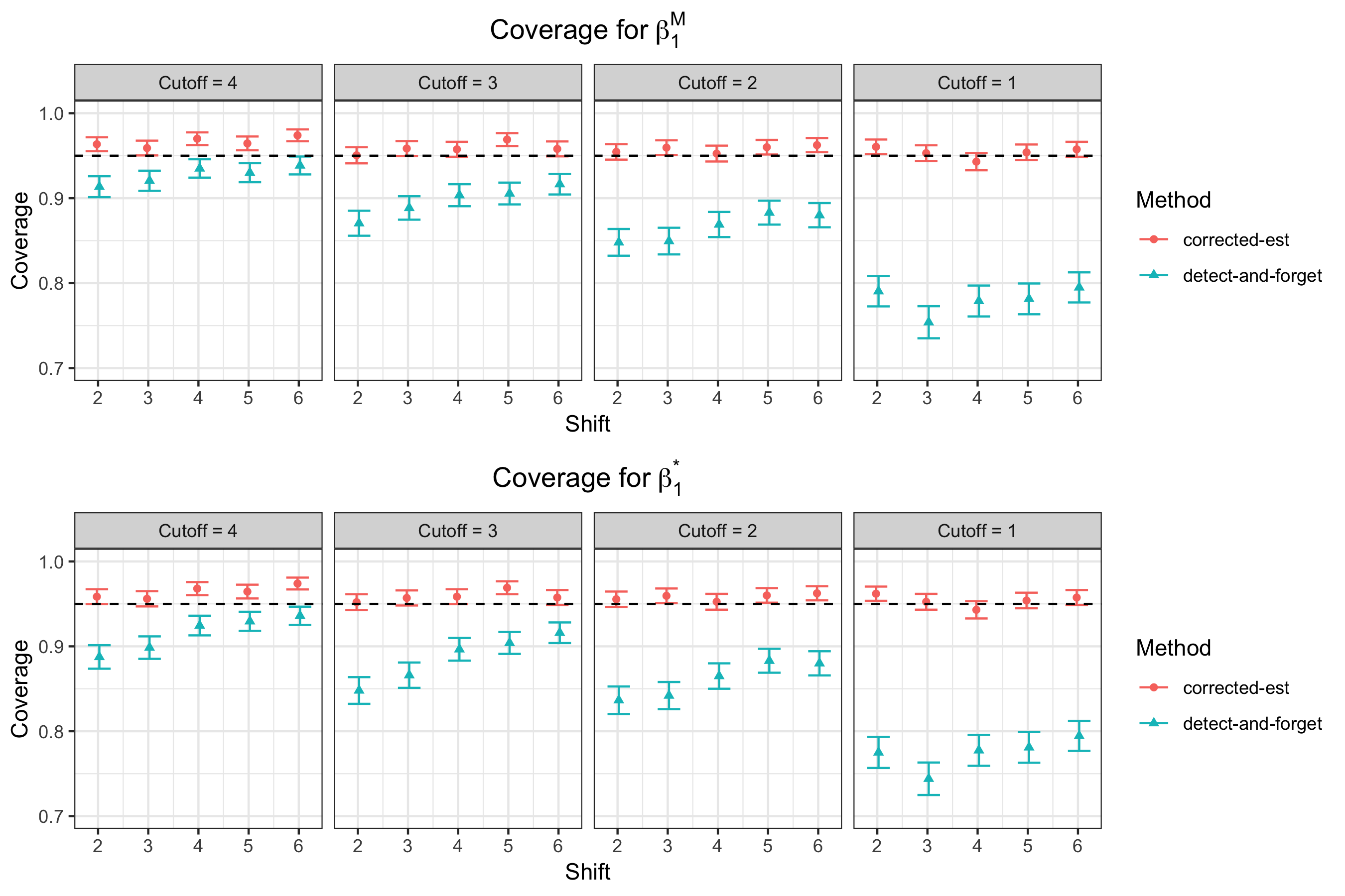
Figure 3: Empirical coverage probability for $\boldsymbol{\beta}^{M}_{1}$ and $\boldsymbol{\beta}^{*}_{1}$. The error bar of coverage probability is obtained by $\hat{q}\pm 1.96\sqrt{\hat{q}(1-\hat{q})/\text{nsim}}$, where $\hat{q}$ is the empirical coverage probability and $\text{nsim}=2000$ is the number of realizations. The dashed line represents $95\%$ coverage.

Figure 4 shows the length of both kinds of intervals. We see that the achievement of desired coverage comes with a price: the length of corrected-est intervals is in general wider than detect-and-forget intervals.

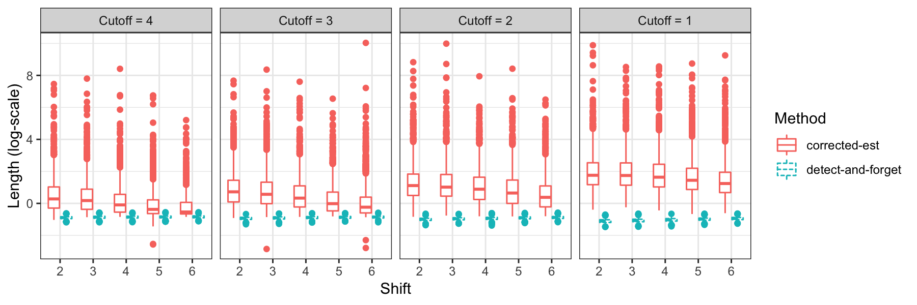
Figure 4: Length of confidence intervals for $\boldsymbol{\beta}^{M}_{1}$.

We next examine the power of testing $H_{0}(M,1):\boldsymbol{\beta}^{M}_{1}=0$ against $H_{1}(M,1):\boldsymbol{\beta}^{M}_{1}\neq 0$. We let $\boldsymbol{\beta}^{*}_{k}=1$ for $k=0,2,3,\ldots,10$, and we vary $\boldsymbol{\beta}^{*}_{1}$ smoothly. We let $s=4$ and the rest of the setup is the same as the previous simulation. We run $2000$ iterations. In each iteration, we generate the response, detect outliers, and extract $p$-values. The detect-and-forget $p$-value is set to be $2F_{t}^{|M|-p}(-|\frac{\boldsymbol{\nu}_{\text{coef}}^{T}\mathbf{y}}{\hat{\sigma}_{\text{REFIT}}\|\boldsymbol{\nu}_{\text{coef}}\|_{2}}|)$, where $F_{t}^{df}$ is the CDF of a $t_{df}$ distribution. For power considerations, corrected-est and corrected-exact $p$-values and are defined as $2\min(1-\text{pval},\text{pval})$, where pval is the $p$-value calculated by directly applying Corollary 3.5 or Theorem 3.9. By construction, we are actually examining the power of testing $H_{0}(*,1):\boldsymbol{\beta}^{*}_{1}=0$ against $H_{1}(*,1):\boldsymbol{\beta}^{*}_{1}\neq 0$. Figure 5 shows the results: the two selective methods control the type I error down to $0.05$ even though this correspond to $H_{0}(*,1)$ (recall that our theory ensures control under $H_{0}(M,1)$), while detect-and-forgetdoes not. Both corrected-est and corrected-exact suffer from a loss of power, although comparing to the power of detect-and-forget is not meaningful since it does not control Type I error. The power for corrected-est seems acceptable, while corrected-exact has quite a substantial loss in power, which may be the consequence of conditioning on too much information.

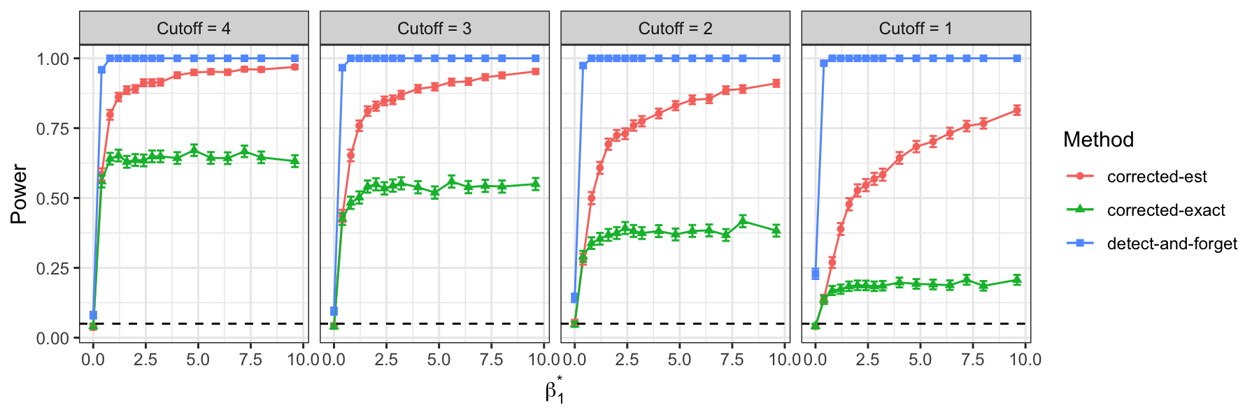
Figure 5: The empirical power of testing $H_{0}(*,1):\boldsymbol{\beta}^{*}_{1}=0$ against $H_{1}(*,1):\boldsymbol{\beta}^{*}_{1}\neq 0$. The error bar is obtained by $\hat{q}\pm 1.96\sqrt{\hat{q}(1-\hat{q})/\text{nsim}}$, where $\hat{q}$ is the empirical power and $\text{nsim}=2000$ is the number of realizations.

We next examine the Type I error and power of testing the global hypothesis $H_{0}(M,g):\boldsymbol{\beta}^{M}_{g}=\mathbf{0}$ against $H_{1}(M,g):\boldsymbol{\beta}^{M}_{g}\neq\mathbf{0}$, where $g=\{1,2,\ldots,10\}$. The setup is the same as the previous simulation, except that we let $\boldsymbol{\beta}^{*}_{0}=1$, $\boldsymbol{\beta}^{*}_{k}=0$ for $k=2,3,\ldots,10$ and we vary $\beta^{*}_{1}$ smoothly. The detect-and-forget $p$-value is set to be $1-{F_{F}^{|g|,|M|-p}(\mathcal{F})},$ where $\mathcal{F}$ is defined in Equation (19) and $F_{F}^{df1,df2}$ is the CDF of an $F_{df1,df2}$ distribution. We examine the power of testing $H_{0}(*,g):\boldsymbol{\beta}^{*}_{g}=\mathbf{0}$ against $H_{1}(*,g):\boldsymbol{\beta}^{*}_{g}\neq\mathbf{0}$. Figure 6 shows the power as a function of $\boldsymbol{\beta}^{*}_{1}$. Again we notice the failure of detect-and-forget method to control the Type I error and the loss of power of the two selective methods.

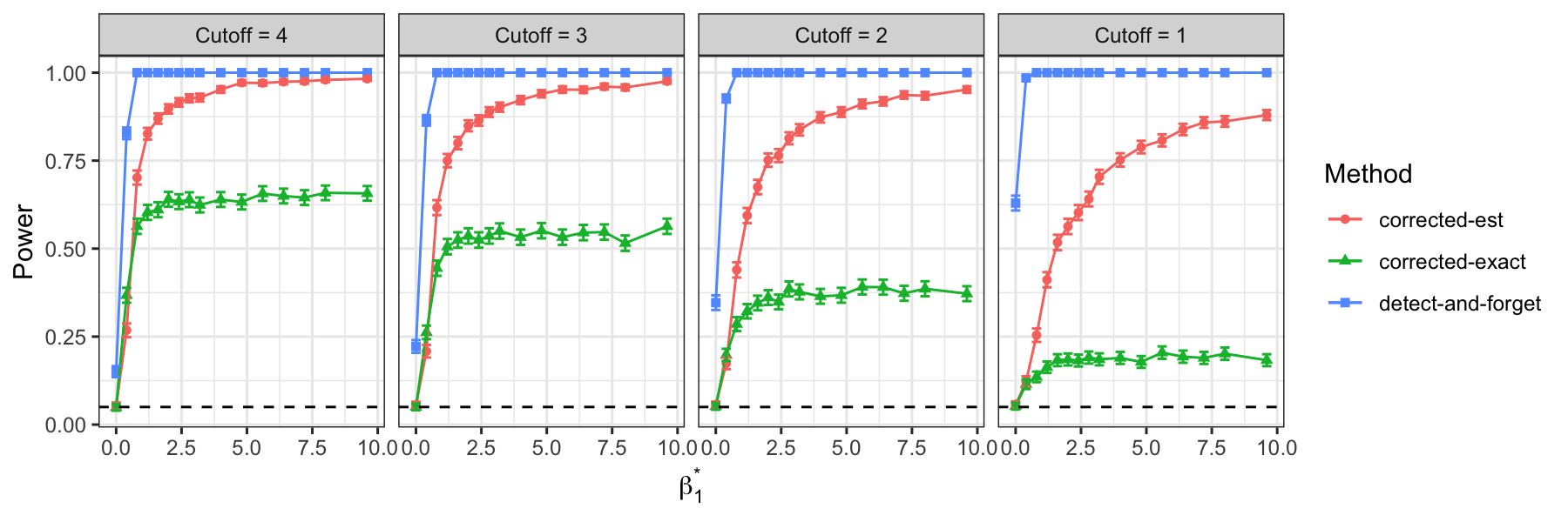
Figure 6: The empirical power of testing $H_{0}(*,g):\boldsymbol{\beta}^{*}_{g}=\mathbf{0}$ against $H_{1}(*,g):\boldsymbol{\beta}^{*}_{g}\neq\mathbf{0}$,The error bar is obtained by $\hat{q}\pm 1.96\sqrt{\hat{q}(1-\hat{q})/\text{nsim}}$, where $\hat{q}$ is the empirical power and $\text{nsim}=2000$ is the number of realizations.

4.2 Data Examples

We next apply our method on three data sets. The first one is a data set from real estate economics, which has $n=7820$ and $p=17$ (Eichholtz et al., 2010). And we apply both corrected-est and corrected-exact to this data set. The other two data sets are classical data sets from the outlier detection literature. Since the number of observations of these two data sets are relatively small, the estimation of $\sigma$ is not be as accurate as in previous simulations, and we only use corrected-exact, despite the fact that we may suffer from a substantial loss of power.

Green Rating Data

This data set consists of $p=17$ covariates of $n=7820$ buildings with places to rent (Eichholtz et al., 2010). The covariates include area of the rental space of the building, the age of the building, and employment growth rating in the building’s geographic region. Due to the page limit, we refer the readers to Section 7 of the online supplementary material for a detailed analysis of this data set, and we only present some highlights here. The most interesting covariate among all $17$ covariates is green_rating, “an indicator for whether the building is either LEED- or Energystar-certified”, i.e., whether the building is a certified green building. A green building is environmentally responsible and resource-efficient throughout its life-cycle (Kibert, 2016). The question investigated in Eichholtz et al. (2010) was the effect of green_rating on the rent charged to tenants in the building.

To do so, we fit a linear model using log-rent as the response and assess the $p$-value associated with green_rating. After inspecting the diagnostic plots, we find that the naive fit (without removing any outliers) gives a model that highly violates the usual linear model assumptions (i.e., normality and homoscedasticity). Hence we use Cook’s distance (with cutoff $\lambda=4$) to detect outliers. This outlier detection procedure identifies $390$ potential outliers, and in view of the sample size, the removal of them should lead to a minimal loss of efficiency. After outlier removal, we consider three methods for constructing $p$-values: detect-and-forget, corrected-est, and corrected-exact. While the detect-and-forget method gives an over-optimistic $p$-value of $4.75\times 10^{-6}$, corrected-est gives $p=0.039$ and corrected-exact gives $p=4.31\times 10^{-4}$. While the two corrected methods give the same conclusion at $\alpha=0.05$, the associated $p$-values are much larger than that given by the naive detect-and-forget method. The $p$-value given by corrected-exact  is smaller than that given by corrected-est. This appears to be due to the lasso regression over-estimating $\sigma$ in this application.

Stack Loss Data

Brownlee’s Stack Loss Plant Data (Brownlee, 1965) involves measures on an industrial plant’s operation and has $21$ observations and three covariates. According to ?stackloss in R (R Core Team, 2017), “Air.Flow is the rate of operation of the plant, Water.Temp is the temperature of cooling water circulated through coils in the absorption tower, and Acid.Conc is the concentration of the acid circulating, minus 50, times 10.” The response, stack.loss, “is an inverse measure of the overall efficiency of the plant.” This data set is considered by many papers in the outlier detection literature (Daniel and Wood, 1999; Atkinson and Atkinson, 1985; Hoeting et al., 1996). The general consensus is that observations $1,3,4$ and $21$ are outliers.

We use Cook’s distance to detect outliers, then fit the model and extract $p$-values, assuming $\sigma$ is unknown. The results are shown in Table 1. We see that as we detect outliers, the adjusted $R^{2}$ increases, which is an indication that the model is getting better. We also notice that corrected-exact $p$-values are in general different from detect-and-forget ones, but there are several cases where the methods’ $p$-values coincide (e.g. Water.Temp with cutoff $4$). This is because the truncation set for the $F$ statistic is $[0,\infty)$ in those cases. This means that outlier removal does not have an effect on the conditional distribution of these test statistics.

Table 1: Inference for each variable in Stack Loss data after outlier detection using Cook’s distance. The $p$-values in bold font are the selective ones, while the other $p$-values are refitted ones.

	Full Fit	Cutoff = 4	Cutoff = 3	Cutoff = 2	Cutoff = 1
Outlier Detected	None	$21$	$1,21$	$1,3,4,21$	$1,2,3,4,7,12,17,21$
Adjusted $R^{2}$	$0.8983$	$0.9392$	$0.9171$	$0.9692$	$0.9057$
Air.Flow: Estimate	$0.7156$	$0.8891$	$0.8458$	$0.7977$	$0.6666$
Air.Flow: $p$-value	$5.8\times 10^{-5}$	$\bf 0.00403$ $1.31\times 10^{-6}$	$\bf 0.345$ $7.7\times 10^{-6}$	$\bf 3.18\times 10^{-4}$ $2.48\times 10^{-8}$	$\bf 0.245$ $1.19\times 10^{-4}$
Water.Temp: Estimate	$1.2953$	$0.8166$	$0.8153$	$0.5773$	$0.6357$
Water.Temp: $p$-value	$0.00263$	$\bf 0.02309$ $0.02309$	$\bf 0.335$ $0.02431$	$\bf 0.00694$ $0.00408$	$\bf 0.792$ $0.01465$
Acid.Conc: Estimate	$-0.1521$	$-0.1071$	$-0.0881$	$-0.0671$	$-0.0411$
Acid.Conc: $p$-value	$0.34405$	$\bf 0.40234$ $0.40234$	$\bf 0.376$ $0.49585$	$\bf 0.2961$ $0.2961$	$\bf 0.208$ $0.653$

Scottish Hill Races Data

This data set records the time for $35$ Scottish hill races in 1984 (Atkinson, 1986). There are two covariates: “dist is the distance in miles, and climb is the total height gained during the route in feet”. The response, time, “is the record time in hours”. This data set is also a classic one considered by many papers in the outlier detection literature (e.g., Atkinson, 1986; Hadi, 1990; Hoeting et al., 1996). The consensus is that observation 7 and 18 are obvious outliers, while observation 33 is an outlier that is masked by the other two outliers.

Again, we use Cook’s distance to detect outliers, then fit the model and extract $p$-values, assuming $\sigma$ is unknown. The results are shown in Table 2. We can see the increase in adjusted $R^{2}$ as outliers are detected, and the corrected-exact $p$-values differ from the detect-and-forget $p$-values in general. Observation $33$ is not detected until the cutoff is set to $1$, and observation $11$ is always detected as an outlier. Atkinson (1986) reports that observations $7,18,11,33,35$ are high-leverage points but argues that only $7,11,33$ are actual outliers, while the others are high-leverage points that agree with the bulk of the data. But we recall that our intent is not to concern ourselves with the accurate detection of outliers but rather with the proper adjustment to inference based on outlier detection and removal.

Table 2: Inference for each variable in Scottish Hill Races data after outlier detection using Cook’s distance. The $p$-values in bold font are the selective ones, while the other $p$-values are refitted ones.

	Full Fit	Cutoff = 4	Cutoff = 3	Cutoff = 2	Cutoff = 1
Outlier Detected	None	$7,11,18$	$7,11,18$	$7,11,18,31$	$7,11,18,31,33,35$
Adjusted $R^{2}$	$0.914$	$0.9721$	$0.9721$	$0.9723$	$0.9395$
dist: Estimate	$0.1036$	$0.1138$	$0.1138$	$0.1111$	$0.1034$
dist: $p$-value	$9.94\times 10^{-12}$	$\bf 1.76\times 10^{-6}$ $6.80\times 10^{-15}$	$\bf 1.06\times 10^{-4}$ $6.80\times 10^{-15}$	$\bf 0.1219$ $6.50\times 10^{-14}$	$\bf 6.99\times 10^{-9}$ $2.13\times 10^{-13}$
climb: Estimate	$1.84\times 10^{-4}$	$1.28\times 10^{-4}$	$1.28\times 10^{-4}$	$1.42\times 10^{-4}$	$1.17\times 10^{-4}$
climb: $p$-value	$6.49\times 10^{-6}$	$\bf 0.05918$ $9.15\times 10^{-6}$	$\bf 0.02465$ $9.15\times 10^{-6}$	$\bf 0.06060$ $1.16\times 10^{-5}$	$\bf 7.02\times 10^{-4}$ $1.53\times 10^{-5}$

5 Discussion

In this paper, we have introduced an inferential framework for properly accounting for the removal of outliers from a data set. The commonplace approach, detect-and-forget, makes the incorrect assumption that outlier removal does not affect the distribution of the data. Our work is based on recent developments in the selective inference literature, which carries out inference that properly accounts for variable selection (Lee et al., 2016; Loftus and Taylor, 2015). A key idea in that work is to characterize the event that a certain set of variables is selected in terms of a simple to describe set of constraints on the response vector $\mathbf{y}$. Doing so makes it tractable to derive the conditional distribution of the estimator given this selection event. Our work likewise relies on the fact that the most commonly used outlier detection procedures can be expressed in a relatively simple form, namely a quadratic constraint on the response vector. Our results can be in principle extended to “convex detection procedures”, where the event $\{\widehat{M}=M\}$ is characterized as a convex constraint on the response, using the results from Harris et al. (2016).

Our target of inference is $\boldsymbol{\beta}^{M}$, where $M$ is the selected set of non-outliers. By focusing on $\boldsymbol{\beta}^{M}$, we are able to decouple the challenge of identifying outliers from the focus of our work, which is accounting for the search and removal of potential outliers. When $M$ excludes all true outliers, $\boldsymbol{\beta}^{M}$ coincides with $\boldsymbol{\beta}^{*}$. When the true outliers are easily detected, then (via Proposition 2.1), our methodology translates to inference on $\boldsymbol{\beta}^{*}$. However, when there are true outliers that are undetected, our statements about $\boldsymbol{\beta}^{M}$ may not translate well to statements on $\beta^{*}$. In some cases, an outlier may not be too severe and therefore go undetected; in such a case, $\boldsymbol{\beta}^{M}$ would not be too far from $\beta^{*}$, in which case our inferential statements may be translated, approximately, to statements about $\boldsymbol{\beta}^{*}$. An interesting future direction would be to characterize the regimes (in terms of size of outlier) in which (i) all true outliers are easily detected and thus we can make inferential statements about $\boldsymbol{\beta}^{*}$ and (ii) not all outliers are easily detected but $\boldsymbol{\beta}^{M}\approx\boldsymbol{\beta}^{*}$ so that approximate statements about $\boldsymbol{\beta}^{*}$ can be made. And of course, a central question would then be whether there is a gap between regimes (i) and (ii).

The inferential framework introduced in this paper suffers from a loss of power, especially in the case of unknown $\sigma$. A possible remedy is to introduce some randomization into the outlier detection procedure. For example, one can adopt the strategy of Tian et al. (2018), namely adding a properly scaled Gaussian noise to the response, so that the selective tests can have a better power at the cost of a less accurate outlier detection procedure. Investigating possible strategies to increase the power remains for future work.

In this paper, we have provided frequentist inference in the linear model after outlier removal. However, with the characterization of the detection procedure at hand, our method can be extended to a Bayesian setup, namely constructing the appropriate detection-adjusted posterior on the regression coefficients, by adapting the results from Yekutieli (2012); Panigrahi et al. (2016).

Another future direction would be to consider proper inference after outlier removal in the high-dimensional setting. Our method explicitly assumes a low-dimensional setting through the assumption that $X_{\widehat{M},\operatorname*{\scalerel*{\cdot}{\bigodot}}}$ has linearly independent columns. A direct generalization of the outlier detection method (8) is to instead solve

$$(\hat{\boldsymbol{\beta}},\hat{\mathbf{u}})=\underset{\boldsymbol{\beta}\in\mathbb{R}^{p},\mathbf{u}\in\mathbb{R}^{n}}{\arg\min}\frac{1}{2n}\|\mathbf{y}-X\beta-\mathbf{u}\|_{2}^{2}+\lambda_{1}\|\boldsymbol{\beta}\|_{1}+\lambda_{2}\|\mathbf{u}\|_{1}.$$

Applying Lee et al. (2016, Theorem 4.3), one could perform inference corrected simultaneously for both variable selection and outlier removal. Another approach would be to use a high-dimensional extension of Cook’s distance proposed by Zhao et al. (2013) (it too can be shown to be a quadratic outlier detection procedure). One could then do variable selection with the remaining data, for example using the lasso. In this case our methodology would still, in principle, apply. Characterizing the exact conditional distributions from more general procedures, such as after MM-estimation, remains a non-trivial problem.

References

- Atkinson (1986) Atkinson, A. (1986). Influential observations, high leverage points, and outliers in linear regression: Comment: Aspects of diagnostic regression analysis. Statistical Science 1(3), 397–402.
- Atkinson and Atkinson (1985) Atkinson, A. C. and A. C. Atkinson (1985). Plots, transformations and regression; an introduction to graphical methods of diagnostic regression analysis. Technical report.
- Belsley et al. (2005) Belsley, D. A., E. Kuh, and R. E. Welsch (2005). Regression diagnostics: Identifying influential data and sources of collinearity, Volume 571. John Wiley & Sons.
- Berenguer-Rico and Nielsen (2017) Berenguer-Rico, R. and B. Nielsen (2017). Marked and weighted empirical processes of residuals with applications to robust regressions. Technical report.
- Berenguer-Rico and Wilms (2018) Berenguer-Rico, V. and I. Wilms (2018). White heteroscedasticty testing after outlier removal. Technical report.
- Bi et al. (2017) Bi, N., J. Markovic, L. Xia, and J. Taylor (2017). Inferactive data analysis. arXiv preprint arXiv:1707.06692.
- Brownlee (1965) Brownlee, K. A. (1965). Statistical theory and methodology in science and engineering, Volume 150. Wiley New York.
- Cook (1977) Cook, R. D. (1977). Detection of influential observation in linear regression. Technometrics 19(1), 15–18.
- Daniel and Wood (1999) Daniel, C. and F. S. Wood (1999). Fitting equations to data: computer analysis of multifactor data. John Wiley & Sons, Inc.
- Eichholtz et al. (2010) Eichholtz, P., N. Kok, and J. M. Quigley (2010). Doing well by doing good? green office buildings. American Economic Review 100(5), 2492–2509.
- Fithian et al. (2014) Fithian, W., D. Sun, and J. Taylor (2014). Optimal inference after model selection. arXiv preprint arXiv:1410.2597.
- Hadi (1990) Hadi, A. (1990). A stepwise procedure for identifying multiple outliers in linear regression. In American Statistical Association Proceedings of the Statistical Computing Section, Volume 137, pp. 142.
- Hadi and Simonoff (1993) Hadi, A. S. and J. S. Simonoff (1993). Procedures for the identification of multiple outliers in linear models. Journal of the American Statistical Association 88(424), 1264–1272.
- Harris et al. (2016) Harris, X. T., S. Panigrahi, J. Markovic, N. Bi, and J. Taylor (2016). Selective sampling after solving a convex problem. arXiv preprint arXiv:1609.05609.
- Hoeting et al. (1996) Hoeting, J., A. E. Raftery, and D. Madigan (1996). A method for simultaneous variable selection and outlier identification in linear regression. Computational Statistics & Data Analysis 22(3), 251–270.
- Huber and Ronchetti (1981) Huber, P. and E. Ronchetti (1981). Robust statistics, ser. Wiley Series in Probability and Mathematical Statistics. New York, NY, USA, Wiley-IEEE 52, 54.
- Huber (1965) Huber, P. J. (1965). A robust version of the probability ratio test. The Annals of Mathematical Statistics, 1753–1758.
- Huber (1992) Huber, P. J. (1992). Robust estimation of a location parameter. In Breakthroughs in statistics, pp. 492–518. Springer.
- Kibert (2016) Kibert, C. J. (2016). Sustainable construction: green building design and delivery. John Wiley & Sons.
- Lee et al. (2016) Lee, J. D., D. L. Sun, Y. Sun, J. E. Taylor, et al. (2016). Exact post-selection inference, with application to the lasso. The Annals of Statistics 44(3), 907–927.
- Loftus and Taylor (2015) Loftus, J. R. and J. E. Taylor (2015). Selective inference in regression models with groups of variables. arXiv preprint arXiv:1511.01478.
- Maronna et al. (2006) Maronna, R., R. D. Martin, and V. Yohai (2006). Robust statistics, Volume 1. John Wiley & Sons, Chichester. ISBN.
- Panigrahi et al. (2016) Panigrahi, S., J. Taylor, and A. Weinstein (2016). Bayesian post-selection inference in the linear model. arXiv preprint arXiv:1605.08824.
- R Core Team (2017) R Core Team (2017). R: A Language and Environment for Statistical Computing. Vienna, Austria: R Foundation for Statistical Computing.
- Reid et al. (2013) Reid, S., R. Tibshirani, and J. Friedman (2013). A study of error variance estimation in lasso regression. arXiv preprint arXiv:1311.5274.
- Rousseeuw (1984) Rousseeuw, P. J. (1984). Least median of squares regression. Journal of the American Statistical Association 79(388), 871–880.
- She and Owen (2011) She, Y. and A. B. Owen (2011). Outlier detection using nonconvex penalized regression. Journal of the American Statistical Association 106(494), 626–639.
- Taylor and Tibshirani (2015) Taylor, J. and R. J. Tibshirani (2015). Statistical learning and selective inference. Proceedings of the National Academy of Sciences 112(25), 7629–7634.
- Thompson (1985) Thompson, R. (1985). A note on restricted maximum likelihood estimation with an alternative outlier model. Journal of the Royal Statistical Society: Series B (Methodological) 47(1), 53–55.
- Tian et al. (2018) Tian, X., J. Taylor, et al. (2018). Selective inference with a randomized response. The Annals of Statistics 46(2), 679–710.
- Tibshirani (1996) Tibshirani, R. (1996). Regression shrinkage and selection via the lasso. Journal of the Royal Statistical Society. Series B (Methodological), 267–288.
- Tibshirani et al. (2017) Tibshirani, R., R. Tibshirani, J. Taylor, J. Loftus, and S. Reid (2017). selectiveInference: Tools for Post-Selection Inference. R package version 1.2.2.
- Welsch and Kuh (1977) Welsch, R. E. and E. Kuh (1977). Linear regression diagnostics.
- Welsh and Ronchetti (2002) Welsh, A. H. and E. Ronchetti (2002). A journey in single steps: robust one-step m-estimation in linear regression. Journal of Statistical Planning and Inference 103(1-2), 287–310.
- Yekutieli (2012) Yekutieli, D. (2012). Adjusted bayesian inference for selected parameters. Journal of the Royal Statistical Society: Series B (Statistical Methodology) 74(3), 515–541.
- Yohai (1987) Yohai, V. J. (1987). High breakdown-point and high efficiency robust estimates for regression. The Annals of Statistics, 642–656.
- Zaman et al. (2001) Zaman, A., P. J. Rousseeuw, and M. Orhan (2001). Econometric applications of high-breakdown robust regression techniques. Economics Letters 71(1), 1–8.
- Zhao et al. (2013) Zhao, J., C. Leng, L. Li, H. Wang, et al. (2013). High-dimensional influence measure. The Annals of Statistics 41(5), 2639–2667.