${\text{CTL}^{*}}$ Synthesis  via  LTL Synthesis

Roderick Bloem1 1 Graz University of Technology, Austria
2 University of Liverpool, UK
   Sven Schewe2 1 Graz University of Technology, Austria
2 University of Liverpool, UK
   Ayrat Khalimov1 1 Graz University of Technology, Austria
2 University of Liverpool, UKThe authors-order was decided by tossing the coin.
Abstract

We reduce synthesis for ${\text{CTL}^{*}}$ properties to synthesis for LTL. In the context of model checking this is impossible — ${\text{CTL}^{*}}$ is more expressive than LTL. Yet, in synthesis we have knowledge of the system structure and we can add new outputs. These outputs can be used to encode witnesses of the satisfaction of ${\text{CTL}^{*}}$ subformulas directly into the system. This way, we construct an LTL formula, over old and new outputs and original inputs, which is realisable if, and only if, the original ${\text{CTL}^{*}}$ formula is realisable. The ${\text{CTL}^{*}}$-via-LTL synthesis approach preserves the problem complexity, although it might increase the minimal system size. We implemented the reduction, and evaluated the ${\text{CTL}^{*}}$-via-LTL synthesiser on several examples.

1 Introduction

In reactive synthesis we automatically construct a system from a given specification in some temporal logic. The problem was introduced by Church for Monadic Second Order Logic [5]. Later Pnueli introduced Linear Temporal Logic (LTL) [16] and together with Rosner proved 2EXPTIME-completeness of the reactive synthesis problem for LTL [17]. In parallel, Emerson and Clarke introduced Computation Tree Logic (CTL) [6], and later Emerson and Halpern introduce Computation Tree Star Logic (${\text{CTL}^{*}}$[7] that subsumes both CTL and LTL. Kupferman and Vardi showed [13] that the synthesis problem for ${\text{CTL}^{*}}$ is 2EXPTIME-complete.

Intuitively, LTL allows one to reason about infinite computations. The logic has temporal operators, e.g., $\operatorname{\mathsf{G}}$ (always) and $\operatorname{\mathsf{F}}$ (eventually), and allows one to state properties like “every request is eventually granted” ($\operatorname{\mathsf{G}}(r\rightarrow\operatorname{\mathsf{F}}g)$). A system satisfies a given LTL property if all its computations satisfy it.

In contrast, CTL and ${\text{CTL}^{*}}$ reason about computation trees, usually derived by unfolding the system. The logics have—in addition to temporal operators—path quantifiers: ${\operatorname{\mathsf{A}}}$ (on all paths) and ${\operatorname{\mathsf{E}}}$ (there exists a path). CTL forbids arbitrary nesting of path quantifiers and temporal operators: they must interleave. E.g., $\operatorname{\mathsf{AG}}g$ (“on all paths we always grant”) is a CTL formula, but $\operatorname{\mathsf{AGF}}g$ (“on all paths we infinitely often grant”) is not a CTL formula. ${\text{CTL}^{*}}$ lifts this limitation.

The expressive powers of CTL and LTL are incomparable: there are systems indistinguishable by CTL but distiniguishable by LTL, and vice versa. One important property inexpressible in LTL is the resettability property: “there is always a way to reach the ‘reset’ state” ($\operatorname{\mathsf{AGEF}}reset$).

There was a time when CTL and LTL competed for “best logic for model checking” [21]. Nowadays most model checkers use LTL. LTL is also prevalent in reactive synthesis. SYNTCOMP [10]—the reactive synthesis competetion with the goal to popularise reactive synthesis—has two distinct tracks, and both use LTL as their specification language.

Yet LTL leaves the designer without structural properties. One solution is to develop general ${\text{CTL}^{*}}$ synthesisers like the one in [11]. Another solution is to transform the ${\text{CTL}^{*}}$ synthesis problem into the form understandable to LTL synthesisers, i.e., to reduce ${\text{CTL}^{*}}$ synthesis to LTL synthesis. Such a reduction would automatically transfer performance advances in LTL synthesisers to a ${\text{CTL}^{*}}$ synthesiser. This paper shows one such reduction.

Our reduction of ${\text{CTL}^{*}}$ synthesis to LTL synthesis works as follows.

First, recall how the standard ${\text{CTL}^{*}}$ model checking works [3]. The verifier introduces a proposition for every state subformula—formulas starting with an ${\operatorname{\mathsf{A}}}$ or an ${\operatorname{\mathsf{E}}}$ path quantifier—of a given ${\text{CTL}^{*}}$ formula. Then the verifier annotates system states with these propositions, in the bottom up fashion, starting with propositions that describe subformulas over original propositions (system inputs and outputs) only. Therefore the system satisfies the ${\text{CTL}^{*}}$ formula iff the initial system state is annotated with the proposition describing the whole ${\text{CTL}^{*}}$ formula (assuming that the ${\text{CTL}^{*}}$ formula starts with ${\operatorname{\mathsf{A}}}$ or ${\operatorname{\mathsf{E}}}$).

Now let us look into ${\text{CTL}^{*}}$ synthesis. The synthesiser has the flexibility to choose the system structure, as long as it satisfies a given specification. We introduce new propositions—outputs that later can be hidden from the user—for state subformulas of the ${\text{CTL}^{*}}$ formula, just like in the model checking case above. We also introduce additional propositions for existentially quantified subformulas—to encode the witnesses of their satisfaction. Such propositions describe the directions (inputs) the system should take to satisfy existentially quantified path formulas. The requirement that new propositions indeed denote the truth of the subformulas can be stated in LTL. For example, for a state subformula ${\operatorname{\mathsf{A}}}\varphi$, we introduce proposition $p_{\_}{{\operatorname{\mathsf{A}}}\varphi}$, and require $\operatorname{\mathsf{G}}\left[p_{\_}{{\operatorname{\mathsf{A}}}\varphi}\rightarrow\varphi^{\prime}\right]$, where $\varphi^{\prime}$ is $\varphi$ with state subformulas substituted by the propositions. For an existential subformula ${\operatorname{\mathsf{E}}}\varphi$, we introduce proposition $p_{\_}{{\operatorname{\mathsf{E}}}\varphi}$ and require, roughly, $\operatorname{\mathsf{G}}\left[p_{\_}{{\operatorname{\mathsf{E}}}\varphi}\rightarrow((\operatorname{\mathsf{G}}d_{\_}{p_{\_}{{\operatorname{\mathsf{E}}}\varphi}})\rightarrow\varphi^{\prime})\right]$, which states: if the proposition $p_{\_}{{\operatorname{\mathsf{E}}}\varphi}$ holds, then the path along directions encoded by $d_{\_}{p_{\_}{{\operatorname{\mathsf{E}}}\varphi}}$ satisfies $\varphi^{\prime}$ (where $\varphi^{\prime}$ as before). We wrote “roughly”, because there can be several different witnesses for the same existential subformula starting at different system states: they may meet in the same system state, but depart afterwards—then, to able to depart from the meeting state, each witness should have its own direction $d$. We show that, for each existential subformula, a number $\approx 2^{|\Phi_{\_}{\text{CTL}^{*}}|}$ of witnesses is sufficient, where $\Phi_{\_}{\text{CTL}^{*}}$ is a given ${\text{CTL}^{*}}$ formula. This makes the LTL formula exponential in the size of the ${\text{CTL}^{*}}$ formula, but the special—conjunctive—nature of the LTL formula ensures that the synthesis complexity is 2EXPTIME wrt. $|\Phi_{\_}{\text{CTL}^{*}}|$.

Our reduction is “if and only if”, and it preserves the synthesis complexity. However, it may increase the size of the system, and is not very well suited to establish unrealisability. Of course, to show that the ${\text{CTL}^{*}}$ formula is unrealisable, one could reduce ${\text{CTL}^{*}}$ synthesis to LTL synthesis, then reduce the LTL synthesis problem to solving parity games, and derive the unrealisability from there111Reducing LTL synthesis to solving parity games is practical, as SYNTCOMP’17 [10] showed: such synthesiser ltlsynt was among the fastest.. But the standard approach for unrealisability checking—by synthesising the dualised LTL specification—does not seem to be practical, since the automaton for the negated LTL formula explodes in size.

Finally, we have implemented222Available at https://github.com/5nizza/party-elli, branch “cav17” the converter from ${\text{CTL}^{*}}$ into LTL, and evaluated ${\text{CTL}^{*}}$-via-LTL synthesis approach, using two LTL synthesisers and ${\text{CTL}^{*}}$ synthesiser [11], on several examples. The experimental results show that such an approach works very well—outperforming the specialised ${\text{CTL}^{*}}$ synthesiser [11]—when the number of ${\text{CTL}^{*}}$-specific formulas is small.

The paper structure is as follows. Section 2 defines Büchi and co-Büchi word automata, tree automata, ${\text{CTL}^{*}}$ with inputs, Moore systems, computation trees, and other useful notions. Section 3 contains the main contribution: it describes the reduction. In Section 4 we briefly discuss checking unrealisability of ${\text{CTL}^{*}}$ specifications. Section 5 describes the experimental setup, specifications, solvers used, and synthesis timings. We conclude in Section 6.

2 Definitions

Notation: $\mathbb{B}=\{\textsf{true},\textsf{false}\}$ is the set of Boolean values, $\mathbb{N}$ is the set of natural numbers (excluding 00), $[i,j]$ for integers $i\leq j$ is the set $\{i,...,j\}$, $[k]$ is $[1,k]$ for $k\in\mathbb{N}$. By default, we use natural numbers.

In this paper we consider finite systems and automata.

2.1 Moore Systems

A (Moore) system $M$ is a tuple $(I,O,T,t_{\_}0,\tau,out)$ where $I$ and $O$ are disjoint sets of input and output variables, $T$ is the set of states, $t_{\_}0\in T$ is the initial state, $\tau:T\times{2^{I}}\to T$ is a transition function, $out:T\to{2^{O}}$ is the output function that labels each state with a set of output variables. Note that systems have no dead ends and have a transition for every input. We write $t\stackrel{{\scriptstyle{io}}}{{\rightarrow}}t^{\prime}$ when $t^{\prime}=\tau(t,i)$ and $out(t)=o$.

For the rest of the section, fix a system $M=(I,O,T,t_{\_}0,\tau,out)$.

A system path is a sequence $t_{\_}1t_{\_}2...\in T^{\omega}$ such that, for every $i$, there is $e\in{2^{I}}$ with $\tau(t_{\_}i,e)=t_{\_}{i+1}$. An input-labeled system path is a sequence $(t_{\_}1,e_{\_}1)(t_{\_}2,e_{\_}2)...\in(T\times{2^{I}})^{\omega}$ where $\tau(t_{\_}i,e_{\_}i)=t_{\_}{i+1}$ for every $i$. A system trace starting from $t_{\_}1\in T$ is a sequence $(o_{\_}1\cup e_{\_}1)(o_{\_}2\cup e_{\_}2)...\in({2^{I}}\cup{2^{O}})^{\omega}$, for which there exists an input-labeled system path $(t_{\_}1,e_{\_}1)(t_{\_}2,e_{\_}2)...$ and $o_{\_}i=out(t_{\_}i)$ for every $i$. Note that, since systems are Moore, the output $o_{\_}i$ cannot “react” to input $e_{\_}i$. I.e., the outputs are “delayed” with respect to inputs.

2.2 Trees

A (infinite) tree is a tuple $(D,L,V\subseteq D^{*},l:V\to L)$, where

  • $D$ is the set of directions,

  • $L$ is the set of node labels,

  • $V$ is the set of nodes satisfying: (i) $\epsilon\in V$ is called the root (the empty sequence), (ii) $V$ is closed under prefix operation (i.e., every node is connected to the root), (iii) for every $n\in V$ there exists $d\in D$ such that $n\cdot d\in V$ (i.e., there are no leafs),

  • $l$ is the nodes labeling function.

A tree $(D,L,V,l)$ is exhaustive iff $V=D^{*}$.

A tree path is a sequence $n_{\_}1n_{\_}2...\in V^{\omega}$, such that, for every $i$, there is $d\in D$ and $n_{\_}{i+1}=n_{\_}i\cdot d$.

In contexts where $I$ and $O$ are inputs and outputs, we call an exhaustive tree $(D={2^{I}},L={2^{O}},V=D^{*},l:V\to{2^{O}})$ a computation tree. We omit $D$ and $L$ when they are clear from the context. E.g. we can write $(V=(2^{I})^{*},l:V\to 2^{O})$ instead of $({2^{I}},{2^{O}},V=(2^{I})^{*},l:V\to{2^{O}})$.

With every system $M=(I,O,T,t_{\_}0,\tau,out)$ we associate the computation tree $(D,L,V,l)$ such that, for every $n\in V$: $l(n)=out(\tau(t_{\_}0,n))$, where $\tau(t_{\_}0,n)$ is the state, in which the system, starting in the initial state $t_{\_}0$, ends after reading the input word $n$. We call such a tree a system computation tree.

A computation tree is regular iff it is a system computation tree for some system.

2.3 ${\text{CTL}^{*}}$ with Inputs (release PNF) and LTL

For this section, fix two disjoint sets: inputs $I$ and outputs $O$. Below we define ${\text{CTL}^{*}}$ with inputs (in release positive normal form). The definition differentiates inputs and outputs (see Remark 1).

Syntax of ${\text{CTL}^{*}}$ with inputs. State formulas have the grammar:

$$\Phi=\textsf{true}\mid\textsf{false}\mid o\mid\neg o\mid\Phi\land\Phi\mid\Phi\lor\Phi\mid{\operatorname{\mathsf{A}}}\varphi\mid{\operatorname{\mathsf{E}}}\varphi$$

where $o\in O$ and $\varphi$ is a path formula. Path formulas are defined by the grammar:

$$\varphi=\Phi\mid i\mid\neg i\mid\varphi\land\varphi\mid\varphi\lor\varphi\mid\operatorname{\mathsf{X}}\varphi\mid\varphi\mathbin{\mathsf{U}}\varphi\mid\varphi\mathbin{\mathsf{R}}\varphi,$$

where $i\in I$. The temporal operators $\operatorname{\mathsf{G}}$ and $\operatorname{\mathsf{F}}$ are defined as usual.

The above grammar describes the ${\text{CTL}^{*}}$ formulas in positive normal form. The general ${\text{CTL}^{*}}$ formula (in which negations can appear anywhere) can be converted into the formula of this form with no size blowup, using equivalence $\neg(a\mathbin{\mathsf{U}}b)\equiv\neg a\mathbin{\mathsf{R}}\neg b$.

Semantics of ${\text{CTL}^{*}}$ with inputs. We define the semantics of ${\text{CTL}^{*}}$ with respect to a computation tree $(V,l)$. The definition is very similar to the standard one [3], except for a few cases involving inputs (marked with “+”).

Let $n\in V$ and $o\in O$. Then:

  • $n\not\models\Phi$ iff $n\models\Phi$ does not hold

  • $n\models\textsf{true}$ and $n\not\models\textsf{false}$

  • $n\models o$ iff $o\in l(n)$, $n\models\neg o$ iff $o\not\in l(n)$

  • $n\models\Phi_{\_}1\land\Phi_{\_}2$ iff $n\models\Phi_{\_}1$ and $n\models\Phi_{\_}2$. Similarly for $\Phi_{\_}1\lor\Phi_{\_}2$.

  • +

    $n\models{\operatorname{\mathsf{A}}}\varphi$ iff for all tree paths $\pi$ starting from $n$: $\pi\models\varphi$. For ${\operatorname{\mathsf{E}}}\varphi$, replace “for all” with “there exists”.

Let $\pi=n_{\_}1n_{\_}2...\in V^{\omega}$ be a tree path, $i\in I$, and $n_{\_}2=n_{\_}1\cdot e$ where $e\in 2^{I}$. For $k\in\mathbb{N}$, define $\pi_{\_}{[k:]}=n_{\_}kn_{\_}{k+1}...$, i.e., the suffix of $\pi$ starting in $n_{\_}k$. Then:

  • $\pi\models\Phi$ iff $n_{\_}1\models\Phi$

  • +

    $\pi\models i$ iff $i\in e$, $\pi\models\neg i$ iff $i\not\in e$. Note how inputs are shifted wrt. outputs.

  • $\pi\models\varphi_{\_}1\land\varphi_{\_}2$ iff $\pi\models\varphi_{\_}1$ and $\pi\models\varphi_{\_}2$. Similarly for $\varphi_{\_}1\lor\varphi_{\_}2$.

  • $\pi\models\operatorname{\mathsf{X}}\varphi$ iff $\pi_{\_}{[2:]}\models\varphi$

  • $\pi\models\varphi_{\_}1\mathbin{\mathsf{U}}\varphi_{\_}2$ iff $\exists l\in\mathbb{N}:(\pi_{\_}{[l:]}\models\varphi_{\_}2\land\forall m\in[1,l-1]:\pi_{\_}{[m:]}\models\varphi_{\_}1)$

  • $\pi\models\varphi_{\_}1\mathbin{\mathsf{R}}\varphi_{\_}2$ iff $(\forall l\in\mathbb{N}:\pi_{\_}{[l:]}\models\varphi_{\_}2)\lor(\exists l\in\mathbb{N}:\pi_{\_}{[l:]}\models\varphi_{\_}1\land\forall m\in[1,l]:\pi_{\_}{[m:]}\models\varphi_{\_}2)$

A computation tree $(V,l)$ satisfies a ${\text{CTL}^{*}}$ state formula $\Phi$, written $(V,l)\models\Phi$, iff the root node satisfies it. A system $M$ satisfies a ${\text{CTL}^{*}}$ state formula $\Phi$, written $M\models\Phi$, iff its computation tree satisfies it.

Remark 1 (Subtleties).

Note that $(V,l)\models i\land o$ is not defined, since $i\land o$ is not a state formula. Let $r\in I$ and $g\in O$. By the semantics, ${\operatorname{\mathsf{E}}}r\equiv\textsf{true}$ and ${\operatorname{\mathsf{E}}}\neg r\equiv\textsf{true}$, while ${\operatorname{\mathsf{E}}}g\equiv g$ and ${\operatorname{\mathsf{E}}}\neg g\equiv\neg g$. This are the consequences of how we group inputs with outputs.

LTL. The syntax of LTL formula (in general form) is:

$$\phi=\textsf{true}\mid\textsf{false}\mid p\mid\neg p\mid\phi\land\phi\mid\neg\phi\mid\phi\mathbin{\mathsf{U}}\phi\mid\operatorname{\mathsf{X}}\phi,$$

where $p\in I\cup O$. Temporal operators $\operatorname{\mathsf{G}}$ and $\operatorname{\mathsf{F}}$ are defined as usual. The semantics is standard (see e.g. [3]), and can be derived from that of ${\text{CTL}^{*}}$ assuming that $\pi\models\neg\phi$ iff $\pi\not\models\phi$. A computation tree $(V,l)$ satisfies an LTL formula $\phi$, written $(V,l)\models\phi$, iff all tree paths starting in the root satisfy it. A system satisfies an LTL formula iff its computation tree satisfies it.

2.4 Word Automata

A word automaton $A$ is a tuple $(\Sigma,Q,q_{\_}0,\delta,acc)$ where $\Sigma$ is an alphabet, $Q$ is a set of states, $q_{\_}0\in Q$ is the initial state, $\delta:Q\times\Sigma\to 2^{Q}\smallsetminus\{\emptyset\}$ is a transition relation, $acc:Q^{\omega}\to\mathbb{B}$ is a path acceptance condition. Note that word automata have no dead ends and have a transition for every letter of the alphabet. A word automaton is deterministic when $|\delta(q,\sigma)|=1$ for every $(q,\sigma)\in Q\times\Sigma$.

For the rest of this section, fix word automaton $A=(\Sigma,Q,q_{\_}0,\delta,acc)$ with $\Sigma=2^{I\cup O}$.

A path in automaton $A$ is a sequence $q_{\_}1q_{\_}2...\in Q^{\omega}$ such that there exists $a_{\_}i\in\Sigma$ for every $i$ such that $(q_{\_}i,a_{\_}i,q_{\_}{i+1})\in\delta(q_{\_}i)$. A word $a_{\_}1a_{\_}2...\in\Sigma^{\omega}$ generates a path $\pi=q_{\_}1\dots$ iff for every $i$: $(q_{\_}i,a_{\_}i,q_{\_}{i+1})\in\delta$. A path $\pi$ is accepted iff $acc(\pi)$ holds.

We define two acceptance conditions. Let $\pi\in Q^{\omega}$, $\textit{Inf}(\pi)$ be the elements of $Q$ appearing in $\pi$ infinitely often, and $F\subseteq Q$. Then:

  • Büchi acceptance: $acc(\pi)$ holds iff $\textit{Inf}(\pi)\cap F\neq\emptyset$.

  • co-Büchi acceptance: $acc(\pi)$ holds iff $\textit{Inf}(\pi)\cap F=\emptyset$.

We distinguish two types of word automata: universal and non-deterministic ones. A nondeterministic word automaton $A$ accepts a word from $\Sigma^{\omega}$ iff there exists an accepted path generated by the word that starts in an initial state. Universal word automata require all such paths to be accepted.

Abbreviations. NBW means nondeterministic Büchi automaton, and UCW means universal co-Büchi automaton.

2.5 Synthesis Problem

The ${\text{CTL}^{*}}$ synthesis problem is:

Given: the set of inputs $I$, the set of outputs $O$, ${\text{CTL}^{*}}$ formula $\Phi$
Return: a computation tree satisfying $\Phi$, otherwise “unrealisable”

The inputs to the problem are called a specification. A specification is realisable if the answer is a tree, and then the tree is called a model of the specification. Similarly we can define the LTL synthesis problem.

It is known [13, 17] that the ${\text{CTL}^{*}}$ and LTL synthesis problems are 2EXPTIME-complete, and any realisable specification has a regular computation tree model.

2.6 Tree Automata

This paper can be understood without complete understanding of alternating tree automata, but since they are mentioned in several places, we define them here. Namely, below we define alternating hesitant tree automata [14], which describe ${\text{CTL}^{*}}$ formulas, similarly to how NBWs describe LTL formulas. The difference is due to the mix of $\operatorname{\mathsf{E}}$ and $\operatorname{\mathsf{A}}$ path quantifiers—hesitant tree automata have an acceptance condition that mixes Büchi and co-Büchi acceptance conditions and certain structural properties.

We start with a general case of alternating tree automata and then define alternating hesitant tree automata.

For a finite set $S$, let ${\cal B}^{+}(S)$ denote the set of all positive Boolean formulas over elements of $S$.

Alternating Tree Automata

An alternating tree automaton is a tuple $(\Sigma,D,Q,q_{\_}0,\delta,acc)$, where $\Sigma$ is the set of node propositions, $D$ is the set of directions, $q_{\_}0\subseteq Q$ is the initial state, $\delta:Q\times\Sigma\to\mathcal{B}^{+}(D\times Q)$ is the transition relation, and $acc$ is an acceptance condition $acc:Q^{\omega}\to\mathbb{B}$. Note that $\delta(q,\sigma)\neq\textsf{false}$ for every $(q,\sigma)\in Q\times\Sigma$, i.e., there is always a transition. Tree automata consume exhaustive trees like $(D,L=\Sigma,V=D^{*},l:V\to\Sigma)$ and produce run-trees.

Fix two disjoint sets, inputs $I$ and outputs $O$.

Run-tree of an alternating tree automaton $(\Sigma=2^{O},D=2^{I},Q,q_{\_}0,\delta,acc)$ on a computation tree $(V=(2^{I})^{*},l:V\to{2^{O}})$ is a tree with directions $2^{I}\times Q$, labels $V\times Q$, nodes $V^{\prime}\subseteq(2^{I}\times Q)^{*}$, labeling function $l^{\prime}$ such that

  • $l^{\prime}(\epsilon)=(\epsilon,q_{\_}0)$,

  • if $v\in V^{\prime}$ with $l^{\prime}(v)=(n,q)$, then:
    there exists $\{(d_{\_}1,q_{\_}1),...,(d_{\_}k,q_{\_}k)\}$ that satisfies $\delta(q,l(n))$ and $n\cdot(d_{\_}i,q_{\_}i)\in V^{\prime}$ for every $i\in[1,k]$.

Intuitively, we run the alternating tree automaton on the computation tree:

  • (1)

    We mark the root node of the computation tree with the automaton initial state $q_{\_}0$. We say that initially, in the node $\epsilon$, there is only one copy of the automaton and it has state $q_{\_}0$.

  • (2)

    We read the label $l(n)$ of the current node $n$ of the computation tree and consult the transition function $\delta(q,l(n))$. The latter gives a set of conjuncts of atoms of the form $(d^{\prime},q^{\prime})\in D\times Q$. We nondeterministically choose one such conjunction $\{(d_{\_}1,q_{\_}1),...,(d_{\_}k,q_{\_}k)\}$ and send a copy of the alternating automaton into each direction $e_{\_}i$ in the state $q_{\_}i$. Note that we can send up to $|Q|$ copies of the automaton into one direction (but into different automaton states). That is why a run-tree defined above has directions $2^{I}\times Q$ rather than $2^{I}$.

  • (3)

    We repeat step (2) for every copy of the automaton. As a result we get a run-tree: the tree labeled with nodes of the computation tree and states of the automaton.

A run-tree is accepting iff every run-tree path starting from the root is accepting. A run-tree path $v_{\_}1v_{\_}2...$ is accepting iff $acc(q_{\_}1q_{\_}2...)$ holds ($acc$ is defined later), where $q_{\_}i$ for every $i\in\mathbb{N}$ is the automaton state part of $l^{\prime}(v_{\_}i)$.

An alternating tree automaton $A=(\Sigma=2^{O},D=2^{I},Q,q_{\_}0,\delta,acc)$ accepts a computation tree $(V=(2^{I})^{*},l:V\to{2^{O}})$, written $(V,l)\models A$, iff the automaton has an accepting run-tree on that computation tree. An alternating tree automaton is non-empty iff there exists a computation tree accepted by it.

Similarly, a Moore system $M=(I,O,T,t_{\_}0,\tau,out)$ is accepted by the alternating tree automaton $A=(\Sigma=2^{O},D=2^{I},Q,q_{\_}0,\delta,acc)$, written $M\models A$, iff $(V,l)\models A$, where $(V=(2^{I})^{*},l:V\to 2^{O})$ is the system computation tree.

Different variations of acceptance conditions are defined the same way as for word automata.

We can define nondeterministic and universal tree automata in a way similar to word automata.

Alternating Hesitant Tree Automata (AHT)

An alternating hesitant tree automaton (AHT) is an alternating tree automaton $(\Sigma,D,Q,q_{\_}0,\delta,acc)$ with the following acceptance condition and structural restrictions. The restrictions reflect the fact that AHTs are tailored for ${\text{CTL}^{*}}$ formulas.

  • $Q$ can be partitioned into $Q^{N}_{\_}1,\dots,Q^{N}_{\_}{k_{\_}N}$, $Q^{U}_{\_}1,\dots,Q^{U}_{\_}{k_{\_}U}$, where superscript $N$ means nondeterministic and $U$ means universal. Let $Q^{N}=\bigcup Q^{N}_{\_}i$ and $Q^{U}=\bigcup Q^{U}_{\_}i$. (Intuitively, nondeterministic state sets describe $\operatorname{\mathsf{E}}$-quantified subformulas of the ${\text{CTL}^{*}}$ formula, while universal — $\operatorname{\mathsf{A}}$-quantified subformulas.)

  • There is a partial order on $\{Q^{N}_{\_}1,\dots,Q^{N}_{\_}{k_{\_}N},Q^{U}_{\_}1,\dots,Q^{U}_{\_}{k_{\_}U}\}$. (Intuitively, this is because state subformulas can be ordered according to their relative nesting.)

  • The transition function $\delta$ satisfies: for every $q\in Q$, $a\in\Sigma$

    • if $q\in Q^{N}_{\_}i$, then: $\delta(q,a)$ contains only disjunctively related111In a Boolean formula, atoms $E$ are disjunctively [conjunctively] related iff the formula can be written into DNF [CNF] in such a way that each cube [clause] has at most one element from $E$. elements of $Q^{N}_{\_}i$; every element of $\delta(q,a)$ outside of $Q^{N}_{\_}i$ belongs to a lower set;

    • if $q\in Q^{U}_{\_}i$, then: $\delta(q,a)$ contains only conjunctively related111In a Boolean formula, atoms $E$ are disjunctively [conjunctively] related iff the formula can be written into DNF [CNF] in such a way that each cube [clause] has at most one element from $E$. elements of $Q^{U}_{\_}i$; every element of $\delta(q,a)$ outside of $Q^{U}_{\_}i$ belongs to a lower set.

Finally, $acc:Q^{\omega}\to\mathbb{B}$ of AHTs is defined by a set $Acc\subseteq Q$: $acc(\pi)$ holds for $\pi=q_{\_}1q_{\_}2...\in Q^{\omega}$ iff one of the following holds.

  • The sequence $\pi$ is trapped in some $Q^{U}_{\_}i$ and $\textit{Inf}(\pi)\cap(Acc\cap Q^{U})=\emptyset$ (co-Büchi acceptance).

  • The sequence $\pi$ is trapped in some $Q^{N}_{\_}i$ and $\textit{Inf}(\pi)\cap(Acc\cap Q^{N})\neq\emptyset$ (Büchi acceptance).

An example of an alternating hesitant tree automaton is in Figure 1.

3 Converting ${\text{CTL}^{*}}$ to LTL for Synthesis

In this section, we describe how and why we can reduce ${\text{CTL}^{*}}$ synthesis to LTL synthesis. First, we recall the standard approach to ${\text{CTL}^{*}}$ synthesis, then describe, step by step, the reduction and the correctness argument, and then discuss some properties of the reduction.

LTL Encoding

Let us first look at standard automata based algorithms for ${\text{CTL}^{*}}$ synthesis [13]. When synthesising a system that realizes a ${\text{CTL}^{*}}$ specification, we normally

  • Turn the ${\text{CTL}^{*}}$ formula into an alternating hesitant tree automaton $A$.

  • We move from computation trees to annotated computation trees that move the (memoryless) strategy of the verifier333Such a strategy maps, in each tree node, an automaton state to a next automaton state and direction. into the label of the computation tree. This allows for using the derived universal co-Büchi tree automaton $U$, making the verifier deterministic: it does not make any decisions, as they are now encoded into the system.

  • We determinise $U$ to a deterministic tree automaton $D$.

  • We play an emptiness game for $D$.

  • If the verifier wins, his winning strategy (after projection of the additional labels) defines a system, if the spoiler wins, the specification is unrealisable.

We draw from this construction and use particular properties of the alternating hesitant tree automaton $A$. Namely, $A$ is not a general alternating tree automaton, but is an alternating hesitant tree automaton. Such an automaton is built from a mix of nondeterministic Büchi and universal co-Büchi word automata, called “existential word automata” and “universal word automata”. These universal and existential word automata start at any system state [tree node] where a universally and existentially, respectively, quantified subformula is marked as true in the annotated model [annotated computation tree]. We use the term “existential word automata” to emphasise that the automaton is not only a non-deterministic word automaton, but it is also used in the alternating tree automaton in a way, where the verifier can pick the system [tree] path along which it has to accept.

Example 1 (Word and tree automata).

Consider formula $\operatorname{\mathsf{EG}}\operatorname{\mathsf{EX}}(g\land\operatorname{\mathsf{X}}(g\land\operatorname{\mathsf{F}}\neg g))$ where the propositions consist of the single output $g$ and the single input $r$. Figure 1 shows non-deterministic word automata for the subformulas, and the alternating (actually, nondeterministic) tree automaton for the whole formula. In what follows, we work mostly with word automata.

$q_{\_}0$\pgfmathresultpt$q_{\_}1$ $q_{\_}2$ $q_{\_}3$ $q_{\_}4$\pgfmathresultpt$1$\pgfmathresultpt$g$\pgfmathresultpt$g$\pgfmathresultpt$g$\pgfmathresultpt$\neg g$\pgfmathresultpt$1$
(a) NBW for $\operatorname{\mathsf{X}}(g\land\operatorname{\mathsf{X}}(g\land\operatorname{\mathsf{F}}\neg g))$, the alphabet $\Sigma$ is $\{r,g\}$. Transitions to the non-final state $sink$ are not shown.
$q_{\_}0^{\prime}$\pgfmathresultpt\pgfmathresultpt$p_{\_}{\operatorname{\mathsf{EX}}}$
(b) NBW for $\operatorname{\mathsf{G}}(p_{\_}{\operatorname{\mathsf{EX}}})$, the alphabet $\Sigma$ is $\{r,g,p_{\_}{\operatorname{\mathsf{EX}}}\}$. The transition to the non-final state $sink$ is omitted.
${}_{\_}1$ ${}_{\_}{\sf E}$ ${}_{\_}{\sf E}$ ${}_{\_}g$ ${}_{\_}g$ ${}_{\_}{\neg g}$ ${}_{\_}1$ ${}_{\_}{\sf E}$ ${}_{\_}{\sf E}$ ${}_{\_}{\sf E}$ ${}_{\_}{\sf E}$ ${}_{\_}g$ ${}_{\_}{\sf E}$ $q_{\_}0^{\prime}$ $q_{\_}1$ $q_{\_}2$ $q_{\_}3$ $q_{\_}4$
(c) Alternating tree automaton for $\operatorname{\mathsf{EG}}\operatorname{\mathsf{EX}}(g\land\operatorname{\mathsf{X}}(g\land\operatorname{\mathsf{F}}\neg g))$. The green color of the states indicate that they are from the nondeterministic partition of the states (and thus double-circled states are from the Büchi acceptance condition). The edges starting in the filled triangle are connected with $\land$. Edge label ${\operatorname{\mathsf{E}}}$ abbreviates the set of edges, for each tree direction, connected with $\lor$. Thus, the transition from $q^{\prime}_{\_}0$ is $((q^{\prime}_{\_}0,r)\lor(q^{\prime}_{\_}0,\neg r))\land((q_{\_}1,r)\lor(q_{\_}1,\neg r))$. To get an alternating automaton for $\operatorname{\mathsf{AG}}\operatorname{\mathsf{EX}}(...)$, replace in the self-loop edge of $q_{\_}0^{\prime}$ label ${\operatorname{\mathsf{E}}}$ with ${\operatorname{\mathsf{A}}}$, and make the state non-final (these also move the state into the universal partition of the states).
Figure 1: Word and tree automata.

We are going to show, step by step, how and why we can reduce ${\text{CTL}^{*}}$-synthesis to LTL synthesis. The steps are outlined in Figure 2(a).

Refer to caption
(a) The verifier takes a computation tree, universal and existential word automata, and the top-level proposition, that together encode a given ${\text{CTL}^{*}}$ formula. It produces an accepting run tree (if the computation tree satisfies the formula).
Refer to caption
(b) We encode the verifier decisions into annotated computation trees, making the verifier deterministic. Figure 3(b) shows such an annotated computation tree.
Refer to caption
(c) The new annotation is a re-phrasing of the previous one. Figure 4 gives an example.
Refer to caption
(d) We keep directions in the annotation but remove next-states—now the verifier has to choose. Figure 5 gives an example.
Refer to caption
(e) Now the obligation of the verifier can be stated in LTL (or using universal co-Büchi word automata).
Figure 2: Steps in the proof of reduction of ${\text{CTL}^{*}}$ synthesis to LTL synthesis.


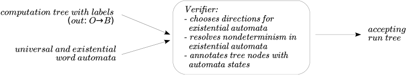
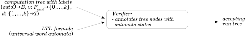
Step A (the starting point). The verifier takes as input: a computation tree, universal and existential word automata for ${\text{CTL}^{*}}$ subformulas, and the top-level proposition corresponding to the whole ${\text{CTL}^{*}}$ formula. It has to produce an accepting run tree (if the computation tree satisfies the formula).

Step B. Given a computation tree, the verifier maps each tree node to an (universal or existential word) automaton state, and moves from a node according to the quantification of the automaton (either in all tree directions or in one direction). The decision, in which tree direction to move and which automaton state to pick for the successor node, constitutes the strategy of the verifier. Each time the verifier has to move in several tree directions (this happens when the node is annotated with a universal word automaton state), we spawn a new version of the verifier, for each tree direction and transition of the universal word automaton.

The strategy of the verifier is a mapping of states of the existential word automata to a decision, which consists of a tree direction (the continuation of the tree path along which the automaton shall accept) and an automaton successor state transition. This is a mapping $dec:Q\rightarrow{2^{I}}\times Q$ such that $dec(q)=(e,q^{\prime})$ implies that $q^{\prime}\in\delta\big{(}q,(l(n),e)\big{)}$, where $\delta$ corresponds to the existential word automaton to which $q$ belongs, and $l(n)\in{2^{O}}$ is a label of the current tree node444The verifier, when in the tree node or system state, moves according to this strategy.. Thus, the strategy is memoryless wrt. the history of automata states. Note that strategies are defined per-node-basis, i.e., they may be different for different nodes.

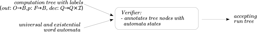
We call a model, in which every state is additionally annotated with a verifier strategy, an annotated model. Similarly, an annotated computation tree is a computation tree in which every node is additionally annotated with a verifier strategy. Thus, in both cases, every system state [node] is labeled with: (i) original propositional labeling $out:O\to\mathbb{B}$, (ii) propositional labeling for universal and existential subformulas $F=F_{\_}\textit{univ}\mathbin{\dot{\cup}}F_{\_}\textit{exist}$, $p:F\to\mathbb{B}$, and (iii) decision labeling $dec:Q\to{2^{I}}\times Q$ where $Q$ are the states of all existential automata.

Example 2.

Figure 3 shows an annotated model and computation tree.

${}_{\_}1$ ${}_{\_}{\sf E}$ ${}_{\_}{\sf E}$ ${}_{\_}g$ ${}_{\_}g$ ${}_{\_}{\neg g}$ ${}_{\_}1$ ${}_{\_}{\sf E}$ ${}_{\_}{\sf E}$ ${}_{\_}{\sf E}$ ${}_{\_}{\sf E}$ ${}_{\_}g$ ${}_{\_}{\sf E}$ $r$ $\bar{r}$ $\bar{r}$ $r$ $q_{\_}0^{\prime}$ $q_{\_}1$ $q_{\_}2$ $q_{\_}3$ $q_{\_}4$ $\bar{g}$ $g$q__0(q_1,r)maps-tosubscriptsubscript𝑞__0subscript𝑞_1𝑟\color[rgb]{0,0,0}\definecolor[named]{pgfstrokecolor}{rgb}{0,0,0}\pgfsys@color@gray@stroke{0}\pgfsys@color@gray@fill{0}{{}_{\_}{q_{\_}0\mapsto(q_{\_}1,r)}}${}_{\_}{q_{\_}0^{\prime}\mapsto(q_{\_}0^{\prime},r)}$q__0(q_1,r)maps-tosubscriptsubscript𝑞__0subscript𝑞_1𝑟\color[rgb]{0,0,0}\definecolor[named]{pgfstrokecolor}{rgb}{0,0,0}\pgfsys@color@gray@stroke{0}\pgfsys@color@gray@fill{0}{{}_{\_}{q_{\_}0\mapsto(q_{\_}1,r)}}${}_{\_}{q_{\_}0^{\prime}\mapsto(q_{\_}0^{\prime},r)}$q__3(q_4,r¯)maps-tosubscriptsubscript𝑞__3subscript𝑞_4¯𝑟\color[rgb]{0,0,0}\definecolor[named]{pgfstrokecolor}{rgb}{0,0,0}\pgfsys@color@gray@stroke{0}\pgfsys@color@gray@fill{0}{{}_{\_}{q_{\_}3\mapsto(q_{\_}4,\bar{r})}}q__1(q_2,r)maps-tosubscriptsubscript𝑞__1subscript𝑞_2𝑟\color[rgb]{0,0,0}\definecolor[named]{pgfstrokecolor}{rgb}{0,0,0}\pgfsys@color@gray@stroke{0}\pgfsys@color@gray@fill{0}{{}_{\_}{q_{\_}1\mapsto(q_{\_}2,r)}}q__2(q_3,r¯)maps-tosubscriptsubscript𝑞__2subscript𝑞_3¯𝑟\color[rgb]{0,0,0}\definecolor[named]{pgfstrokecolor}{rgb}{0,0,0}\pgfsys@color@gray@stroke{0}\pgfsys@color@gray@fill{0}{{}_{\_}{q_{\_}2\mapsto(q_{\_}3,\bar{r})}}q__4(q_4,r¯)maps-tosubscriptsubscript𝑞__4subscript𝑞_4¯𝑟\color[rgb]{0,0,0}\definecolor[named]{pgfstrokecolor}{rgb}{0,0,0}\pgfsys@color@gray@stroke{0}\pgfsys@color@gray@fill{0}{{}_{\_}{q_{\_}4\mapsto(q_{\_}4,\bar{r})}}${}_{\_}{p_{\_}{\sf EX}}$ ${}_{\_}{p_{\_}{\sf EX},p_{\_}{\sf EG}}$
(a) An annotated model satisfying $\operatorname{\mathsf{EG}}\operatorname{\mathsf{EX}}(g\land\operatorname{\mathsf{X}}(g\land\operatorname{\mathsf{F}}\neg g))$. Near the nodes is the winning strategy of the verifier.
${}_{\_}1$ ${}_{\_}{\sf E}$ ${}_{\_}{\sf E}$ ${}_{\_}g$ ${}_{\_}g$ ${}_{\_}{\neg g}$ ${}_{\_}1$ ${}_{\_}{\sf E}$ ${}_{\_}{\sf E}$ ${}_{\_}{\sf E}$ ${}_{\_}{\sf E}$ ${}_{\_}g$ ${}_{\_}{\sf E}$ $r$ $\bar{r}$ $\bar{r}$ $r$ $q_{\_}0^{\prime}$ $q_{\_}1$ $q_{\_}2$ $q_{\_}3$ $q_{\_}4$ $\bar{g}$ $g$q__0(q_1,r)maps-tosubscriptsubscript𝑞__0subscript𝑞_1𝑟\color[rgb]{0,0,0}\definecolor[named]{pgfstrokecolor}{rgb}{0,0,0}\pgfsys@color@gray@stroke{0}\pgfsys@color@gray@fill{0}{{}_{\_}{q_{\_}0\mapsto(q_{\_}1,r)}}${}_{\_}{q_{\_}0^{\prime}\mapsto(q_{\_}0^{\prime},r)}$q__0(q_1,r)maps-tosubscriptsubscript𝑞__0subscript𝑞_1𝑟\color[rgb]{0,0,0}\definecolor[named]{pgfstrokecolor}{rgb}{0,0,0}\pgfsys@color@gray@stroke{0}\pgfsys@color@gray@fill{0}{{}_{\_}{q_{\_}0\mapsto(q_{\_}1,r)}}${}_{\_}{q_{\_}0^{\prime}\mapsto(q_{\_}0^{\prime},r)}$q__3(q_4,r¯)maps-tosubscriptsubscript𝑞__3subscript𝑞_4¯𝑟\color[rgb]{0,0,0}\definecolor[named]{pgfstrokecolor}{rgb}{0,0,0}\pgfsys@color@gray@stroke{0}\pgfsys@color@gray@fill{0}{{}_{\_}{q_{\_}3\mapsto(q_{\_}4,\bar{r})}}q__1(q_2,r)maps-tosubscriptsubscript𝑞__1subscript𝑞_2𝑟\color[rgb]{0,0,0}\definecolor[named]{pgfstrokecolor}{rgb}{0,0,0}\pgfsys@color@gray@stroke{0}\pgfsys@color@gray@fill{0}{{}_{\_}{q_{\_}1\mapsto(q_{\_}2,r)}}q__2(q_3,r¯)maps-tosubscriptsubscript𝑞__2subscript𝑞_3¯𝑟\color[rgb]{0,0,0}\definecolor[named]{pgfstrokecolor}{rgb}{0,0,0}\pgfsys@color@gray@stroke{0}\pgfsys@color@gray@fill{0}{{}_{\_}{q_{\_}2\mapsto(q_{\_}3,\bar{r})}}q__4(q_4,r¯)maps-tosubscriptsubscript𝑞__4subscript𝑞_4¯𝑟\color[rgb]{0,0,0}\definecolor[named]{pgfstrokecolor}{rgb}{0,0,0}\pgfsys@color@gray@stroke{0}\pgfsys@color@gray@fill{0}{{}_{\_}{q_{\_}4\mapsto(q_{\_}4,\bar{r})}}${}_{\_}{p_{\_}{\sf EX}}$ ${}_{\_}{p_{\_}{\sf EX},p_{\_}{\sf EG}}$ $\bar{g}$ $g$ $g$ $\bar{g}$ $\bar{g}$ $g$ $\bar{g}$ $g$ $g$ $\bar{g}$ $g$ $\bar{g}$ $g$ $\bar{g}$ $g$ $\bar{g}$ $\color[rgb]{0,0,1}\definecolor[named]{pgfstrokecolor}{rgb}{0,0,1}{{}_{\_}{q_{\_}0\mapsto(q_{\_}1,r)}}$ ${}_{\_}{q_{\_}0^{\prime}\mapsto(q_{\_}0^{\prime},r)}$ $\color[rgb]{0,0,1}\definecolor[named]{pgfstrokecolor}{rgb}{0,0,1}{{}_{\_}{q_{\_}1\mapsto(q_{\_}2,r)}}$ $\color[rgb]{1,.08,.576}\definecolor[named]{pgfstrokecolor}{rgb}{1,.08,.576}{{}_{\_}{q_{\_}0\mapsto(q_{\_}1,r)}}$ ${}_{\_}{q_{\_}0^{\prime}\mapsto(q_{\_}0^{\prime},r)}$ $\color[rgb]{0,0,1}\definecolor[named]{pgfstrokecolor}{rgb}{0,0,1}{{}_{\_}{q_{\_}2\mapsto(q_{\_}3,r)}}$ $\color[rgb]{1,.08,.576}\definecolor[named]{pgfstrokecolor}{rgb}{1,.08,.576}{{}_{\_}{q_{\_}1\mapsto(q_{\_}2,r)}}$ ${}_{\_}{q_{\_}0^{\prime}\mapsto(q_{\_}0^{\prime},r)}$ $\color[rgb]{1,.08,.576}{}_{\_}{q_{\_}2\mapsto(q_{\_}3,\bar{r})}$ $\color[rgb]{0,0,1}{}_{\_}{q_{\_}3\mapsto(q_{\_}3,\bar{r})}$ ${}_{\_}{q_{\_}0^{\prime}\mapsto(q_{\_}0^{\prime},r)}$ $\color[rgb]{0,.5,0}\definecolor[named]{pgfstrokecolor}{rgb}{0,.5,0}{{}_{\_}{q_{\_}0\mapsto(q_{\_}1,r)}}$ $\color[rgb]{0,.5,0}{}_{\_}{q_{\_}1\mapsto(q_{\_}2,r)}$ $\color[rgb]{.72,.525,.044}\definecolor[named]{pgfstrokecolor}{rgb}{.72,.525,.044}{{}_{\_}{q_{\_}0\mapsto(q_{\_}1,r)}}$ ${}_{\_}{p_{\_}{\sf EX},p_{\_}{\sf EG}}$ ${}_{\_}{p_{\_}{\sf EX}}$ ${}_{\_}{p_{\_}{\sf EX}}$ ${}_{\_}{p_{\_}{\sf EX}}$
(b) An annotated computation tree that satisfies $\operatorname{\mathsf{EG}}\operatorname{\mathsf{EX}}(g\land\operatorname{\mathsf{X}}(g\land\operatorname{\mathsf{F}}\neg g))$. Let proposition $p_{\_}{\operatorname{\mathsf{EG}}}$ correspond to $\operatorname{\mathsf{EG}}(p_{\_}{\operatorname{\mathsf{EX}}})$, and $p_{\_}{\operatorname{\mathsf{EX}}}$—to $\operatorname{\mathsf{EX}}(g\land\operatorname{\mathsf{X}}(g\land\operatorname{\mathsf{F}}\neg g))$. A winning strategy for the verifier is depicted using dashed and colored paths. The black dashed path witnesses $p_{\_}{\operatorname{\mathsf{EG}}}$, the blue path witnesses $p_{\_}{\operatorname{\mathsf{EX}}}$ starting in the root node, the pink path—$p_{\_}{\operatorname{\mathsf{EX}}}$ starting in the left child, and so on. The pink and blue paths share the tail. The annotation for the verifier strategy is on the left side of nodes, and decisions for non mapped states are irrelevant. Note that this particular annotated computation tree is not the unfolding of the annotated model above—here we postpone the right-turn of the blue path in order to illustrate that paths can share the tail.
Figure 3: Annotated model and computation tree.

Step C. The verifier strategy (encoded in the annotated computation tree) encodes both, the words on which the nondeterministic automata are interpreted and witnesses of acceptance (accepting automata paths on those words). For the encoding in LTL that we will later use, it is enough to map out the automaton word, and replace the witnesses by what it actually means: that the automaton word satisfies the respective path formula.

Example 3.

In Figure 3(b), the verifier strategy in the root node maps out the word $(\bar{g},p_{\_}{\operatorname{\mathsf{EX}}},r)(\bar{g},p_{\_}{\operatorname{\mathsf{EX}}},\bar{r})^{\omega}$ on which the NBW in Figure 1(b) is run, and the witness of acceptance $(q^{\prime}_{\_}0)^{\omega}$. The blue path encodes the word $(\bar{g},r)(g,r)(g,r)(g,\bar{r})(\bar{g},\bar{r})^{\omega}$ and the witness $q_{\_}0q_{\_}1q_{\_}2q_{\_}3q_{\_}3q_{\_}4^{\omega}$ for the NBW in Figure 1(a). In total, we can see 5 tree paths that are mapped out by the annotated computation tree.

To map out the word, we look at the set of tree paths that are mapped out in an annotated computation tree and define equivalence classes on them. Two tree paths are equivalent if they share a tail (or, equivalently, if one is the tail of the other).

There is a simple sufficient condition for two mapped out tree paths to be equivalent: if they pass through the same node of the annotated computation tree in the same automaton state, then they have the same future, and are therefore equivalent. 555The condition is sufficient but not necessary. Recall that each mapped out tree path corresponds to at least one copy of the verifier that ensures the path is accepting. When two verifiers go along the same tree path, it can be annotated with different automata states (for example, corresponding to different automata). Then such paths do not satisfy the sufficient condition, although they are trivially equivalent.

Example 4.

In Figure 3(b) the blue and pink paths are equivalent, since they share the tail. The sufficient condition fires in the top node, where the tree paths meet in automaton state $q_{\_}3$

The sufficient condition implies that we cannot have more non-equivalent tree paths passing through a tree node than there are states in all existential word automata; let us call this number $k$. For each tree node, we assign unique numbers from $\{1,...,k\}$ to equivalence classes, and thus any two non-equivalent tree paths that go through the same tree node have different numbers. As this is an intermediate step in our translation, we are wasteful with the labeling:

  • (1)

    we map existential word automata states to numbers (IDs) using a label $id:Q\to\{1,\ldots,k\}$, we choose the direction $d:\{1,\ldots,k\}\to{2^{I}}$ to take, and choose the successor state, $succ:Q\to Q$, such that $succ(q)\in\delta\Big{(}q,\big{(}l(n),d(id(q))\big{)}\Big{)}$, where $l(n)$ is the label of the current node $n$, and

  • (2)

    we maintain the same state ID along the chosen direction: $id(q)=id(succ(q))$.

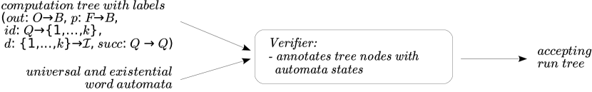
Note that (1) alone can be viewed as a re-phrasing of the labeling $dec$ that we had before on page 2(a). The requirement (2) is satisfiable, because a tree path maintains its equivalence class. Therefore any annotated computation tree can be re-labeled! This step is shown in Figure 2(c), the labels are: $(out:O\to\mathbb{B},p:F\to\mathbb{B},id:Q\to\{1,\ldots,k\},d:\{1,\ldots,k\}\to{2^{I}},succ:Q\to Q)$.

Example 5.

A re-labeled computation tree is in Figure 4.

${}_{\_}1$ ${}_{\_}{\sf E}$ ${}_{\_}{\sf E}$ ${}_{\_}g$ ${}_{\_}g$ ${}_{\_}{\neg g}$ ${}_{\_}1$ ${}_{\_}{\sf E}$ ${}_{\_}{\sf E}$ ${}_{\_}{\sf E}$ ${}_{\_}{\sf E}$ ${}_{\_}g$ ${}_{\_}{\sf E}$ $r$ $\bar{r}$ $\bar{r}$ $r$ $q_{\_}0^{\prime}$ $q_{\_}1$ $q_{\_}2$ $q_{\_}3$ $q_{\_}4$ $\bar{g}$ $g$q__0(q_1,r)maps-tosubscriptsubscript𝑞__0subscript𝑞_1𝑟\color[rgb]{0,0,0}\definecolor[named]{pgfstrokecolor}{rgb}{0,0,0}\pgfsys@color@gray@stroke{0}\pgfsys@color@gray@fill{0}{{}_{\_}{q_{\_}0\mapsto(q_{\_}1,r)}}${}_{\_}{q_{\_}0^{\prime}\mapsto(q_{\_}0^{\prime},r)}$q__0(q_1,r)maps-tosubscriptsubscript𝑞__0subscript𝑞_1𝑟\color[rgb]{0,0,0}\definecolor[named]{pgfstrokecolor}{rgb}{0,0,0}\pgfsys@color@gray@stroke{0}\pgfsys@color@gray@fill{0}{{}_{\_}{q_{\_}0\mapsto(q_{\_}1,r)}}${}_{\_}{q_{\_}0^{\prime}\mapsto(q_{\_}0^{\prime},r)}$q__3(q_4,r¯)maps-tosubscriptsubscript𝑞__3subscript𝑞_4¯𝑟\color[rgb]{0,0,0}\definecolor[named]{pgfstrokecolor}{rgb}{0,0,0}\pgfsys@color@gray@stroke{0}\pgfsys@color@gray@fill{0}{{}_{\_}{q_{\_}3\mapsto(q_{\_}4,\bar{r})}}q__1(q_2,r)maps-tosubscriptsubscript𝑞__1subscript𝑞_2𝑟\color[rgb]{0,0,0}\definecolor[named]{pgfstrokecolor}{rgb}{0,0,0}\pgfsys@color@gray@stroke{0}\pgfsys@color@gray@fill{0}{{}_{\_}{q_{\_}1\mapsto(q_{\_}2,r)}}q__2(q_3,r¯)maps-tosubscriptsubscript𝑞__2subscript𝑞_3¯𝑟\color[rgb]{0,0,0}\definecolor[named]{pgfstrokecolor}{rgb}{0,0,0}\pgfsys@color@gray@stroke{0}\pgfsys@color@gray@fill{0}{{}_{\_}{q_{\_}2\mapsto(q_{\_}3,\bar{r})}}q__4(q_4,r¯)maps-tosubscriptsubscript𝑞__4subscript𝑞_4¯𝑟\color[rgb]{0,0,0}\definecolor[named]{pgfstrokecolor}{rgb}{0,0,0}\pgfsys@color@gray@stroke{0}\pgfsys@color@gray@fill{0}{{}_{\_}{q_{\_}4\mapsto(q_{\_}4,\bar{r})}}${}_{\_}{p_{\_}{\sf EX}}$ ${}_{\_}{p_{\_}{\sf EX},p_{\_}{\sf EG}}$ $\bar{g}$ $g$ $g$ $\bar{g}$ $\bar{g}$ $g$ $\bar{g}$ $g$ $g$ $\bar{g}$ $g$ $\bar{g}$ $g$ $\bar{g}$ $g$ $\bar{g}$ $\color[rgb]{0,0,1}\definecolor[named]{pgfstrokecolor}{rgb}{0,0,1}{{}_{\_}{q_{\_}0\mapsto(q_{\_}1,r)}}$ ${}_{\_}{q_{\_}0^{\prime}\mapsto(q_{\_}0^{\prime},r)}$ $\color[rgb]{0,0,1}\definecolor[named]{pgfstrokecolor}{rgb}{0,0,1}{{}_{\_}{q_{\_}1\mapsto(q_{\_}2,r)}}$ $\color[rgb]{1,.08,.576}\definecolor[named]{pgfstrokecolor}{rgb}{1,.08,.576}{{}_{\_}{q_{\_}0\mapsto(q_{\_}1,r)}}$ ${}_{\_}{q_{\_}0^{\prime}\mapsto(q_{\_}0^{\prime},r)}$ $\color[rgb]{0,0,1}\definecolor[named]{pgfstrokecolor}{rgb}{0,0,1}{{}_{\_}{q_{\_}2\mapsto(q_{\_}3,r)}}$ $\color[rgb]{1,.08,.576}\definecolor[named]{pgfstrokecolor}{rgb}{1,.08,.576}{{}_{\_}{q_{\_}1\mapsto(q_{\_}2,r)}}$ ${}_{\_}{q_{\_}0^{\prime}\mapsto(q_{\_}0^{\prime},r)}$ $\color[rgb]{1,.08,.576}{}_{\_}{q_{\_}2\mapsto(q_{\_}3,\bar{r})}$ $\color[rgb]{0,0,1}{}_{\_}{q_{\_}3\mapsto(q_{\_}3,\bar{r})}$ ${}_{\_}{q_{\_}0^{\prime}\mapsto(q_{\_}0^{\prime},r)}$ $\color[rgb]{0,.5,0}\definecolor[named]{pgfstrokecolor}{rgb}{0,.5,0}{{}_{\_}{q_{\_}0\mapsto(q_{\_}1,r)}}$ $\color[rgb]{0,.5,0}{}_{\_}{q_{\_}1\mapsto(q_{\_}2,r)}$ $\color[rgb]{.72,.525,.044}\definecolor[named]{pgfstrokecolor}{rgb}{.72,.525,.044}{{}_{\_}{q_{\_}0\mapsto(q_{\_}1,r)}}$ ${}_{\_}{p_{\_}{\sf EX},p_{\_}{\sf EG}}$ ${}_{\_}{p_{\_}{\sf EX}}$ ${}_{\_}{p_{\_}{\sf EX}}$ ${}_{\_}{p_{\_}{\sf EX}}$ $\bar{g}$ $g$ $g$ $\bar{g}$ $\bar{g}$ $g$ $\bar{g}$ $g$ $g$ $\bar{g}$ $g$ $\bar{g}$ $g$ $\bar{g}$ $g$ $\bar{g}$ $\color[rgb]{0,0,1}\definecolor[named]{pgfstrokecolor}{rgb}{0,0,1}{{}_{\_}{q_{\_}0\mapsto(1,q_{\_}1),1\mapsto r}}$ $\color[rgb]{0,0,1}\definecolor[named]{pgfstrokecolor}{rgb}{0,0,1}{{}_{\_}{q_{\_}1\mapsto(1,q_{\_}2),1\mapsto r}}$ $\color[rgb]{1,.08,.576}\definecolor[named]{pgfstrokecolor}{rgb}{1,.08,.576}{{}_{\_}{q_{\_}0\mapsto(1,q_{\_}1)~{}~{}~{}~{}~{}}}$ $\color[rgb]{0,0,1}\definecolor[named]{pgfstrokecolor}{rgb}{0,0,1}{{}_{\_}{q_{\_}2\mapsto(1,q_{\_}3),1\mapsto r}}$ $\color[rgb]{1,.08,.576}\definecolor[named]{pgfstrokecolor}{rgb}{1,.08,.576}{{}_{\_}{q_{\_}1\mapsto(1,q_{\_}2)~{}~{}~{}~{}~{}}}$ $\color[rgb]{1,.08,.576}{}_{\_}{q_{\_}2\mapsto(1,q_{\_}3)~{}~{}~{}~{}~{}}$ $\color[rgb]{0,0,1}{}_{\_}{q_{\_}3\mapsto(1,q_{\_}3),1\mapsto\bar{r}}$ $\color[rgb]{0,.5,0}\definecolor[named]{pgfstrokecolor}{rgb}{0,.5,0}{{}_{\_}{q_{\_}0\mapsto(2,q_{\_}1),2\mapsto r}}$ $\color[rgb]{0,.5,0}{}_{\_}{q_{\_}1\mapsto(2,q_{\_}2),2\mapsto r}$ $\color[rgb]{.72,.525,.044}\definecolor[named]{pgfstrokecolor}{rgb}{.72,.525,.044}{{}_{\_}{q_{\_}0\mapsto(3,q_{\_}1),3\mapsto r}}$q__0(4,q_0),4rformulae-sequencemaps-tosubscriptsubscript𝑞__superscript04subscript𝑞_superscript0maps-to4𝑟\color[rgb]{0,0,0}\definecolor[named]{pgfstrokecolor}{rgb}{0,0,0}\pgfsys@color@gray@stroke{0}\pgfsys@color@gray@fill{0}{{}_{\_}{q_{\_}0^{\prime}\mapsto(4,q_{\_}0^{\prime}),4\mapsto r}}q__0(4,q_0),4rformulae-sequencemaps-tosubscriptsubscript𝑞__superscript04subscript𝑞_superscript0maps-to4𝑟\color[rgb]{0,0,0}\definecolor[named]{pgfstrokecolor}{rgb}{0,0,0}\pgfsys@color@gray@stroke{0}\pgfsys@color@gray@fill{0}{{}_{\_}{q_{\_}0^{\prime}\mapsto(4,q_{\_}0^{\prime}),4\mapsto r}}q__0(4,q_0),4rformulae-sequencemaps-tosubscriptsubscript𝑞__superscript04subscript𝑞_superscript0maps-to4𝑟\color[rgb]{0,0,0}\definecolor[named]{pgfstrokecolor}{rgb}{0,0,0}\pgfsys@color@gray@stroke{0}\pgfsys@color@gray@fill{0}{{}_{\_}{q_{\_}0^{\prime}\mapsto(4,q_{\_}0^{\prime}),4\mapsto r}}q__0(4,q_0),4rformulae-sequencemaps-tosubscriptsubscript𝑞__superscript04subscript𝑞_superscript0maps-to4𝑟\color[rgb]{0,0,0}\definecolor[named]{pgfstrokecolor}{rgb}{0,0,0}\pgfsys@color@gray@stroke{0}\pgfsys@color@gray@fill{0}{{}_{\_}{q_{\_}0^{\prime}\mapsto(4,q_{\_}0^{\prime}),4\mapsto r}}${}_{\_}{p_{\_}{\sf EX},p_{\_}{\sf EG}}$ ${}_{\_}{p_{\_}{\sf EX}}$ ${}_{\_}{p_{\_}{\sf EX}}$ ${}_{\_}{p_{\_}{\sf EX}}$
Figure 4: A re-labeled computation tree. Notation “$q_{\_}0\mapsto(1,q_{\_}1)$” means $id(q_{\_}0)=1$ and $succ(q_{\_}0)=q_{\_}1$, and “$1\mapsto r$” means $d$ maps $1$ to $\{r\}$. Since the blue and pink paths are equivalent, the label $id$ maps the corresponding automata states in the nodes to the same number, $1$. The IDs of the green and yellow paths differ implying that they are not equivalent and hence do not share the tail (their tails cannot be seen in the figure).

Step D. In the new annotation with labels $(out,p,id,d,succ)$, labeling $d$ alone maps out the tree path for each ID. The remainder of the information is mainly there to establish that the corresponding word is accepted by the respective word automaton (equivalently: satisfies the respective path formula). If we use only $d$, then the only missing information is where the path starts and which path formula it belongs to—the information originally encoded by $p$.

We address these two points by using numbered computation trees. Recall that the annotated computation trees have a propositional labeling $p:F\to\mathbb{B}$ that labels nodes with subformulas. In the numbered computation trees, we replace $p$ for existential subformulas $F_{\_}\textit{exist}\subseteq F$ by labeling ${v:F_{\_}\textit{exist}\to\{0,...,k\}}$, where, for an existentially quantified formula ${\operatorname{\mathsf{E}}}\varphi\in F_{\_}\textit{exist}$ and a tree node $n$:

  • $v_{\_}{{\operatorname{\mathsf{E}}}\varphi}(n)=0$ encodes that no claim that ${\operatorname{\mathsf{E}}}\varphi$ holds is made (similar to the proposition $p_{\_}{{\operatorname{\mathsf{E}}}\varphi}$ being “false” in the annotated tree), whereas

  • a value $v_{\_}{{\operatorname{\mathsf{E}}}\varphi}(n)\in\{1,...,k\}$ is interpreted similarly to the proposition $p_{\_}{{\operatorname{\mathsf{E}}}\varphi}$ being “true”, but also requires that a witness for ${\operatorname{\mathsf{E}}}\varphi$ is encoded on the tree path that starts in $n$ and follows directions $d_{\_}{v_{\_}{{\operatorname{\mathsf{E}}}\varphi}(n)}$.

Example 6.

The tree in Figure 4 becomes a numbered computation tree if we replace the propositional labels $p_{\_}{\operatorname{\mathsf{EX}}}$ and $p_{\_}{\operatorname{\mathsf{EG}}}$ with ID numbers as follows. The root node has $v_{\_}{\operatorname{\mathsf{EX}}}=1$ and $v_{\_}{\operatorname{\mathsf{EG}}}=4$, the left child has $v_{\_}{\operatorname{\mathsf{EX}}}=1$, the left-left child has $v_{\_}{\operatorname{\mathsf{EX}}}=2$, the left-left-left child has $v_{\_}{\operatorname{\mathsf{EX}}}=3$. Note that $id(q_{\_}0)=v_{\_}{\operatorname{\mathsf{EX}}}$ and $id(q_{\_}0^{\prime})=v_{\_}{\operatorname{\mathsf{EG}}}$ whenever those $v$s are non-zero. The nodes outside of the dashed path have $v_{\_}{\operatorname{\mathsf{EX}}}=v_{\_}{\operatorname{\mathsf{EG}}}=0$, meaning that no claims about satisfaction of the path formulas has to be witnessed there.

Initially, we use ID labeling $v$ in addition with ($out,id,d,succ,p^{\textit{univ}}$), where $p^{\textit{univ}}$ is a restriction of $p$ on $F_{\_}\textit{univ}$, and then there is no relevant change in the way the (deterministic) verifier works. I.e., a numbered computation tree can be turned into annotated computation tree, and vice versa, such that the numbered tree is accepted iff the annotated tree is accepted.
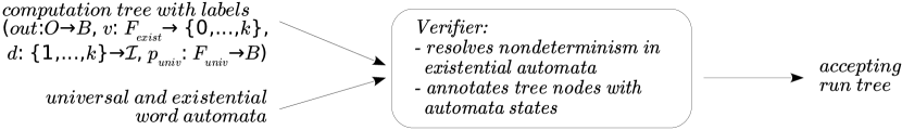
${}_{\_}1$ ${}_{\_}{\sf E}$ ${}_{\_}{\sf E}$ ${}_{\_}g$ ${}_{\_}g$ ${}_{\_}{\neg g}$ ${}_{\_}1$ ${}_{\_}{\sf E}$ ${}_{\_}{\sf E}$ ${}_{\_}{\sf E}$ ${}_{\_}{\sf E}$ ${}_{\_}g$ ${}_{\_}{\sf E}$ $r$ $\bar{r}$ $\bar{r}$ $r$ $q_{\_}0^{\prime}$ $q_{\_}1$ $q_{\_}2$ $q_{\_}3$ $q_{\_}4$ $\bar{g}$ $g$q__0(q_1,r)maps-tosubscriptsubscript𝑞__0subscript𝑞_1𝑟\color[rgb]{0,0,0}\definecolor[named]{pgfstrokecolor}{rgb}{0,0,0}\pgfsys@color@gray@stroke{0}\pgfsys@color@gray@fill{0}{{}_{\_}{q_{\_}0\mapsto(q_{\_}1,r)}}${}_{\_}{q_{\_}0^{\prime}\mapsto(q_{\_}0^{\prime},r)}$q__0(q_1,r)maps-tosubscriptsubscript𝑞__0subscript𝑞_1𝑟\color[rgb]{0,0,0}\definecolor[named]{pgfstrokecolor}{rgb}{0,0,0}\pgfsys@color@gray@stroke{0}\pgfsys@color@gray@fill{0}{{}_{\_}{q_{\_}0\mapsto(q_{\_}1,r)}}${}_{\_}{q_{\_}0^{\prime}\mapsto(q_{\_}0^{\prime},r)}$q__3(q_4,r¯)maps-tosubscriptsubscript𝑞__3subscript𝑞_4¯𝑟\color[rgb]{0,0,0}\definecolor[named]{pgfstrokecolor}{rgb}{0,0,0}\pgfsys@color@gray@stroke{0}\pgfsys@color@gray@fill{0}{{}_{\_}{q_{\_}3\mapsto(q_{\_}4,\bar{r})}}q__1(q_2,r)maps-tosubscriptsubscript𝑞__1subscript𝑞_2𝑟\color[rgb]{0,0,0}\definecolor[named]{pgfstrokecolor}{rgb}{0,0,0}\pgfsys@color@gray@stroke{0}\pgfsys@color@gray@fill{0}{{}_{\_}{q_{\_}1\mapsto(q_{\_}2,r)}}q__2(q_3,r¯)maps-tosubscriptsubscript𝑞__2subscript𝑞_3¯𝑟\color[rgb]{0,0,0}\definecolor[named]{pgfstrokecolor}{rgb}{0,0,0}\pgfsys@color@gray@stroke{0}\pgfsys@color@gray@fill{0}{{}_{\_}{q_{\_}2\mapsto(q_{\_}3,\bar{r})}}q__4(q_4,r¯)maps-tosubscriptsubscript𝑞__4subscript𝑞_4¯𝑟\color[rgb]{0,0,0}\definecolor[named]{pgfstrokecolor}{rgb}{0,0,0}\pgfsys@color@gray@stroke{0}\pgfsys@color@gray@fill{0}{{}_{\_}{q_{\_}4\mapsto(q_{\_}4,\bar{r})}}${}_{\_}{p_{\_}{\sf EX}}$ ${}_{\_}{p_{\_}{\sf EX},p_{\_}{\sf EG}}$ $\bar{g}$ $g$ $g$ $\bar{g}$ $\bar{g}$ $g$ $\bar{g}$ $g$ $g$ $\bar{g}$ $g$ $\bar{g}$ $g$ $\bar{g}$ $g$ $\bar{g}$ $\color[rgb]{0,0,1}\definecolor[named]{pgfstrokecolor}{rgb}{0,0,1}{{}_{\_}{q_{\_}0\mapsto(q_{\_}1,r)}}$ ${}_{\_}{q_{\_}0^{\prime}\mapsto(q_{\_}0^{\prime},r)}$ $\color[rgb]{0,0,1}\definecolor[named]{pgfstrokecolor}{rgb}{0,0,1}{{}_{\_}{q_{\_}1\mapsto(q_{\_}2,r)}}$ $\color[rgb]{1,.08,.576}\definecolor[named]{pgfstrokecolor}{rgb}{1,.08,.576}{{}_{\_}{q_{\_}0\mapsto(q_{\_}1,r)}}$ ${}_{\_}{q_{\_}0^{\prime}\mapsto(q_{\_}0^{\prime},r)}$ $\color[rgb]{0,0,1}\definecolor[named]{pgfstrokecolor}{rgb}{0,0,1}{{}_{\_}{q_{\_}2\mapsto(q_{\_}3,r)}}$ $\color[rgb]{1,.08,.576}\definecolor[named]{pgfstrokecolor}{rgb}{1,.08,.576}{{}_{\_}{q_{\_}1\mapsto(q_{\_}2,r)}}$ ${}_{\_}{q_{\_}0^{\prime}\mapsto(q_{\_}0^{\prime},r)}$ $\color[rgb]{1,.08,.576}{}_{\_}{q_{\_}2\mapsto(q_{\_}3,\bar{r})}$ $\color[rgb]{0,0,1}{}_{\_}{q_{\_}3\mapsto(q_{\_}3,\bar{r})}$ ${}_{\_}{q_{\_}0^{\prime}\mapsto(q_{\_}0^{\prime},r)}$ $\color[rgb]{0,.5,0}\definecolor[named]{pgfstrokecolor}{rgb}{0,.5,0}{{}_{\_}{q_{\_}0\mapsto(q_{\_}1,r)}}$ $\color[rgb]{0,.5,0}{}_{\_}{q_{\_}1\mapsto(q_{\_}2,r)}$ $\color[rgb]{.72,.525,.044}\definecolor[named]{pgfstrokecolor}{rgb}{.72,.525,.044}{{}_{\_}{q_{\_}0\mapsto(q_{\_}1,r)}}$ ${}_{\_}{p_{\_}{\sf EX},p_{\_}{\sf EG}}$ ${}_{\_}{p_{\_}{\sf EX}}$ ${}_{\_}{p_{\_}{\sf EX}}$ ${}_{\_}{p_{\_}{\sf EX}}$ $\bar{g}$ $g$ $g$ $\bar{g}$ $\bar{g}$ $g$ $\bar{g}$ $g$ $g$ $\bar{g}$ $g$ $\bar{g}$ $g$ $\bar{g}$ $g$ $\bar{g}$ $\color[rgb]{0,0,1}\definecolor[named]{pgfstrokecolor}{rgb}{0,0,1}{{}_{\_}{q_{\_}0\mapsto(1,q_{\_}1),1\mapsto r}}$ $\color[rgb]{0,0,1}\definecolor[named]{pgfstrokecolor}{rgb}{0,0,1}{{}_{\_}{q_{\_}1\mapsto(1,q_{\_}2),1\mapsto r}}$ $\color[rgb]{1,.08,.576}\definecolor[named]{pgfstrokecolor}{rgb}{1,.08,.576}{{}_{\_}{q_{\_}0\mapsto(1,q_{\_}1)~{}~{}~{}~{}~{}}}$ $\color[rgb]{0,0,1}\definecolor[named]{pgfstrokecolor}{rgb}{0,0,1}{{}_{\_}{q_{\_}2\mapsto(1,q_{\_}3),1\mapsto r}}$ $\color[rgb]{1,.08,.576}\definecolor[named]{pgfstrokecolor}{rgb}{1,.08,.576}{{}_{\_}{q_{\_}1\mapsto(1,q_{\_}2)~{}~{}~{}~{}~{}}}$ $\color[rgb]{1,.08,.576}{}_{\_}{q_{\_}2\mapsto(1,q_{\_}3)~{}~{}~{}~{}~{}}$ $\color[rgb]{0,0,1}{}_{\_}{q_{\_}3\mapsto(1,q_{\_}3),1\mapsto\bar{r}}$ $\color[rgb]{0,.5,0}\definecolor[named]{pgfstrokecolor}{rgb}{0,.5,0}{{}_{\_}{q_{\_}0\mapsto(2,q_{\_}1),2\mapsto r}}$ $\color[rgb]{0,.5,0}{}_{\_}{q_{\_}1\mapsto(2,q_{\_}2),2\mapsto r}$ $\color[rgb]{.72,.525,.044}\definecolor[named]{pgfstrokecolor}{rgb}{.72,.525,.044}{{}_{\_}{q_{\_}0\mapsto(3,q_{\_}1),3\mapsto r}}$q__0(4,q_0),4rformulae-sequencemaps-tosubscriptsubscript𝑞__superscript04subscript𝑞_superscript0maps-to4𝑟\color[rgb]{0,0,0}\definecolor[named]{pgfstrokecolor}{rgb}{0,0,0}\pgfsys@color@gray@stroke{0}\pgfsys@color@gray@fill{0}{{}_{\_}{q_{\_}0^{\prime}\mapsto(4,q_{\_}0^{\prime}),4\mapsto r}}q__0(4,q_0),4rformulae-sequencemaps-tosubscriptsubscript𝑞__superscript04subscript𝑞_superscript0maps-to4𝑟\color[rgb]{0,0,0}\definecolor[named]{pgfstrokecolor}{rgb}{0,0,0}\pgfsys@color@gray@stroke{0}\pgfsys@color@gray@fill{0}{{}_{\_}{q_{\_}0^{\prime}\mapsto(4,q_{\_}0^{\prime}),4\mapsto r}}q__0(4,q_0),4rformulae-sequencemaps-tosubscriptsubscript𝑞__superscript04subscript𝑞_superscript0maps-to4𝑟\color[rgb]{0,0,0}\definecolor[named]{pgfstrokecolor}{rgb}{0,0,0}\pgfsys@color@gray@stroke{0}\pgfsys@color@gray@fill{0}{{}_{\_}{q_{\_}0^{\prime}\mapsto(4,q_{\_}0^{\prime}),4\mapsto r}}q__0(4,q_0),4rformulae-sequencemaps-tosubscriptsubscript𝑞__superscript04subscript𝑞_superscript0maps-to4𝑟\color[rgb]{0,0,0}\definecolor[named]{pgfstrokecolor}{rgb}{0,0,0}\pgfsys@color@gray@stroke{0}\pgfsys@color@gray@fill{0}{{}_{\_}{q_{\_}0^{\prime}\mapsto(4,q_{\_}0^{\prime}),4\mapsto r}}${}_{\_}{p_{\_}{\sf EX},p_{\_}{\sf EG}}$ ${}_{\_}{p_{\_}{\sf EX}}$ ${}_{\_}{p_{\_}{\sf EX}}$ ${}_{\_}{p_{\_}{\sf EX}}$ $\bar{g}$ $g$ $g$ $\bar{g}$ $\bar{g}$ $g$ $\bar{g}$ $g$ $g$ $\bar{g}$ $g$ $\bar{g}$ $g$ $\bar{g}$ $g$ $\bar{g}$1_r\color[rgb]{0,0,0}\definecolor[named]{pgfstrokecolor}{rgb}{0,0,0}\pgfsys@color@gray@stroke{0}\pgfsys@color@gray@fill{0}{{}_{\_}{1\mapsto r}}4_r\color[rgb]{0,0,0}\definecolor[named]{pgfstrokecolor}{rgb}{0,0,0}\pgfsys@color@gray@stroke{0}\pgfsys@color@gray@fill{0}{{}_{\_}{4\mapsto r}}${}_{\_}{{\color[rgb]{0,0,1}\definecolor[named]{pgfstrokecolor}{rgb}{0,0,1}{v_{\_}{\sf EX}=1}},v_{\_}{\sf EG}=4}$4_r\color[rgb]{0,0,0}\definecolor[named]{pgfstrokecolor}{rgb}{0,0,0}\pgfsys@color@gray@stroke{0}\pgfsys@color@gray@fill{0}{{}_{\_}{4\mapsto r}}1_r\color[rgb]{0,0,0}\definecolor[named]{pgfstrokecolor}{rgb}{0,0,0}\pgfsys@color@gray@stroke{0}\pgfsys@color@gray@fill{0}{{}_{\_}{1\mapsto r}}${}_{\_}{{\color[rgb]{1,.08,.576}\definecolor[named]{pgfstrokecolor}{rgb}{1,.08,.576}{v_{\_}{\sf EX}=1}}}$4_r\color[rgb]{0,0,0}\definecolor[named]{pgfstrokecolor}{rgb}{0,0,0}\pgfsys@color@gray@stroke{0}\pgfsys@color@gray@fill{0}{{}_{\_}{4\mapsto r}}${}_{\_}{{\color[rgb]{0,.5,0}\definecolor[named]{pgfstrokecolor}{rgb}{0,.5,0}{v_{\_}{\sf EX}=2}}}$1_r\color[rgb]{0,0,0}\definecolor[named]{pgfstrokecolor}{rgb}{0,0,0}\pgfsys@color@gray@stroke{0}\pgfsys@color@gray@fill{0}{{}_{\_}{1\mapsto r}}2_r\color[rgb]{0,0,0}\definecolor[named]{pgfstrokecolor}{rgb}{0,0,0}\pgfsys@color@gray@stroke{0}\pgfsys@color@gray@fill{0}{{}_{\_}{2\mapsto r}}4_r\color[rgb]{0,0,0}\definecolor[named]{pgfstrokecolor}{rgb}{0,0,0}\pgfsys@color@gray@stroke{0}\pgfsys@color@gray@fill{0}{{}_{\_}{4\mapsto r}}${}_{\_}{{\color[rgb]{.72,.525,.044}\definecolor[named]{pgfstrokecolor}{rgb}{.72,.525,.044}{v_{\_}{\sf EX}=3}}}$1_r¯\color[rgb]{0,0,0}\definecolor[named]{pgfstrokecolor}{rgb}{0,0,0}\pgfsys@color@gray@stroke{0}\pgfsys@color@gray@fill{0}{{}_{\_}{1\mapsto\bar{r}}}2_r\color[rgb]{0,0,0}\definecolor[named]{pgfstrokecolor}{rgb}{0,0,0}\pgfsys@color@gray@stroke{0}\pgfsys@color@gray@fill{0}{{}_{\_}{2\mapsto r}}3_r\color[rgb]{0,0,0}\definecolor[named]{pgfstrokecolor}{rgb}{0,0,0}\pgfsys@color@gray@stroke{0}\pgfsys@color@gray@fill{0}{{}_{\_}{3\mapsto r}}
Figure 5: Numbered computation tree with redundant annotations removed.

Now we observe that labeling $id$ and $succ$ are used only to witness that each word mapped out by $d$ is accepted by respective existential word automata. I.e., $id$ and $succ$ make the verifier deterministic. Let us remove $id$ and $succ$ from the labeling. We call such trees lean-numbered computation trees; they have labeling $(out:O\to\mathbb{B},v:F_{\_}\textit{exist}\to\{0,...,k\},d:\{1,...,k\}\to{2^{I}},p^{\textit{univ}}:F_{\_}\textit{univ}\to\mathbb{B})$. This makes the verifier nondeterministic. We still have the property: every accepting annotated computation tree can be turned into an accepting lean-numbered computation tree, and vice versa. This step is shown in Figure 2(d); an example of a lean-numbered computation tree is in Figure 5.

Step E (the final step). We show how labeling $(out,v,d,p^{\textit{univ}})$ allows for using LTL formulas instead of directly using automata for the acceptance check. The encoding into LTL is as follows.

  • For each existentially quantified formula ${\operatorname{\mathsf{E}}}\varphi$, we introduce the following LTL formula (recall that $v_{\_}{{\operatorname{\mathsf{E}}}\varphi}=0$ encodes that we do not claim that ${\operatorname{\mathsf{E}}}\varphi$ holds in the current tree node, and $v_{\_}{{\operatorname{\mathsf{E}}}\varphi}\neq 0$ means that ${\operatorname{\mathsf{E}}}\varphi$ does hold and $\varphi$ holds if we follow $v_{\_}{{\operatorname{\mathsf{E}}}\varphi}$-numbered directions):

    $$\bigwedge_{\_}{j\in\{1,...,k\}}\operatorname{\mathsf{G}}\Big{[}v_{\_}{{\operatorname{\mathsf{E}}}\varphi}=j~{}\rightarrow~{}\big{(}\operatorname{\mathsf{G}}d_{\_}j\rightarrow\varphi^{\prime}\big{)}\Big{]},$$ (1)

    where $\varphi^{\prime}$ is obtained from $\varphi$ by replacing the subformulas of the form ${\operatorname{\mathsf{E}}}\psi$ by $v_{\_}{{\operatorname{\mathsf{E}}}\psi}\neq 0$ and the subformulas of the form ${\operatorname{\mathsf{A}}}\psi$ by $p_{\_}{{\operatorname{\mathsf{A}}}\psi}$.

  • For each subformula of the form ${\operatorname{\mathsf{A}}}\varphi$, we simply take

    $$\operatorname{\mathsf{G}}\Big{[}p_{\_}{{\operatorname{\mathsf{A}}}\varphi}~{}\rightarrow~{}\varphi^{\prime}\Big{]},$$ (2)

    where $\varphi^{\prime}$ is obtained from $\varphi$ as before.

  • Finally, the overall LTL formula is the conjunction

    Φ_𝖤φF_existEq.1_𝖠φF_univEq.2superscriptΦsubscript_𝖤𝜑subscript𝐹_existEq.1subscript_𝖠𝜑subscript𝐹_univEq.2\boxed{\Phi^{\prime}\land\bigwedge_{\_}{{\operatorname{\mathsf{E}}}\varphi\in F_{\_}\textit{exist}}\text{Eq.}\ref{eq:ltl-existential}~{}\land\bigwedge_{\_}{{\operatorname{\mathsf{A}}}\varphi\in F_{\_}\textit{univ}}\text{Eq.}\ref{eq:ltl-universal}} (3)

    where the Boolean formula $\Phi^{\prime}$ is obtained by replacing in the original ${\text{CTL}^{*}}$ formula every ${\operatorname{\mathsf{E}}}\varphi$ by $v_{\_}{{\operatorname{\mathsf{E}}}\varphi}\neq 0$ and every ${\operatorname{\mathsf{A}}}\varphi$ by $p_{\_}{{\operatorname{\mathsf{A}}}\varphi}$.

Example 7.

Let $I=\{r\}$, $O=\{g\}$. Consider the CTL formula

$$\operatorname{\mathsf{EG}}\neg g\land\operatorname{\mathsf{AG}}\operatorname{\mathsf{EF}}\neg g\land\operatorname{\mathsf{EF}}g.$$

The sum of states of individual NBWs is $5$ (assuming the natural translations), so we introduce integer propositions $v_{\_}{\operatorname{\mathsf{EF}}\!\bar{g}}$, $v_{\_}{\operatorname{\mathsf{EG}}\!\bar{g}}$, $v_{\_}{\operatorname{\mathsf{EF}}\!g}$, ranging over $\{0,...,5\}$, and five Boolean propositions $d_{\_}1$, …, $d_{\_}5$; we also introduce Boolean proposition $p_{\_}{\operatorname{\mathsf{AG}}(v_{\_}{\operatorname{\mathsf{EF}}\!\bar{g}}\neq 0)}$. The LTL formula is:

$\displaystyle~{}~{}~{}v_{\_}{\operatorname{\mathsf{EG}}\!\bar{g}}\neq 0\land p_{\_}{\operatorname{\mathsf{AG}}(v_{\_}{\operatorname{\mathsf{EF}}\!\bar{g}}\neq 0)}\land v_{\_}{\operatorname{\mathsf{EF}}\!g}\neq 0~{}\land$
$\displaystyle~{}~{}~{}\operatorname{\mathsf{G}}\left[p_{\_}{\operatorname{\mathsf{AG}}(v_{\_}{\operatorname{\mathsf{EF}}\!\bar{g}}\neq 0)}\rightarrow\operatorname{\mathsf{G}}(v_{\_}{\operatorname{\mathsf{EF}}\!\bar{g}}\neq 0)\right]~{}\land$
$\displaystyle\bigwedge_{\_}{j\in\{1...5\}}\operatorname{\mathsf{G}}\left[\begin{aligned} &v_{\_}{\operatorname{\mathsf{EF}}\!\bar{g}}=j~{}\rightarrow~{}(\operatorname{\mathsf{G}}d_{\_}j\rightarrow\operatorname{\mathsf{F}}\neg g)\\ &v_{\_}{\operatorname{\mathsf{EG}}\!\bar{g}}=j~{}\rightarrow~{}(\operatorname{\mathsf{G}}d_{\_}j\rightarrow\operatorname{\mathsf{G}}\neg g)\\ &v_{\_}{\operatorname{\mathsf{EF}}\!g}=j~{}\rightarrow~{}(\operatorname{\mathsf{G}}d_{\_}j\rightarrow\operatorname{\mathsf{F}}g)\end{aligned}\right]$

Figure 6 shows a model satisfying the LTL specification.

${}_{\_}1$ ${}_{\_}{\sf E}$ ${}_{\_}{\sf E}$ ${}_{\_}g$ ${}_{\_}g$ ${}_{\_}{\neg g}$ ${}_{\_}1$ ${}_{\_}{\sf E}$ ${}_{\_}{\sf E}$ ${}_{\_}{\sf E}$ ${}_{\_}{\sf E}$ ${}_{\_}g$ ${}_{\_}{\sf E}$ $r$ $\bar{r}$ $\bar{r}$ $r$ $q_{\_}0^{\prime}$ $q_{\_}1$ $q_{\_}2$ $q_{\_}3$ $q_{\_}4$ $\bar{g}$ $g$q__0(q_1,r)maps-tosubscriptsubscript𝑞__0subscript𝑞_1𝑟\color[rgb]{0,0,0}\definecolor[named]{pgfstrokecolor}{rgb}{0,0,0}\pgfsys@color@gray@stroke{0}\pgfsys@color@gray@fill{0}{{}_{\_}{q_{\_}0\mapsto(q_{\_}1,r)}}${}_{\_}{q_{\_}0^{\prime}\mapsto(q_{\_}0^{\prime},r)}$q__0(q_1,r)maps-tosubscriptsubscript𝑞__0subscript𝑞_1𝑟\color[rgb]{0,0,0}\definecolor[named]{pgfstrokecolor}{rgb}{0,0,0}\pgfsys@color@gray@stroke{0}\pgfsys@color@gray@fill{0}{{}_{\_}{q_{\_}0\mapsto(q_{\_}1,r)}}${}_{\_}{q_{\_}0^{\prime}\mapsto(q_{\_}0^{\prime},r)}$q__3(q_4,r¯)maps-tosubscriptsubscript𝑞__3subscript𝑞_4¯𝑟\color[rgb]{0,0,0}\definecolor[named]{pgfstrokecolor}{rgb}{0,0,0}\pgfsys@color@gray@stroke{0}\pgfsys@color@gray@fill{0}{{}_{\_}{q_{\_}3\mapsto(q_{\_}4,\bar{r})}}q__1(q_2,r)maps-tosubscriptsubscript𝑞__1subscript𝑞_2𝑟\color[rgb]{0,0,0}\definecolor[named]{pgfstrokecolor}{rgb}{0,0,0}\pgfsys@color@gray@stroke{0}\pgfsys@color@gray@fill{0}{{}_{\_}{q_{\_}1\mapsto(q_{\_}2,r)}}q__2(q_3,r¯)maps-tosubscriptsubscript𝑞__2subscript𝑞_3¯𝑟\color[rgb]{0,0,0}\definecolor[named]{pgfstrokecolor}{rgb}{0,0,0}\pgfsys@color@gray@stroke{0}\pgfsys@color@gray@fill{0}{{}_{\_}{q_{\_}2\mapsto(q_{\_}3,\bar{r})}}q__4(q_4,r¯)maps-tosubscriptsubscript𝑞__4subscript𝑞_4¯𝑟\color[rgb]{0,0,0}\definecolor[named]{pgfstrokecolor}{rgb}{0,0,0}\pgfsys@color@gray@stroke{0}\pgfsys@color@gray@fill{0}{{}_{\_}{q_{\_}4\mapsto(q_{\_}4,\bar{r})}}${}_{\_}{p_{\_}{\sf EX}}$ ${}_{\_}{p_{\_}{\sf EX},p_{\_}{\sf EG}}$ $\bar{g}$ $g$ $g$ $\bar{g}$ $\bar{g}$ $g$ $\bar{g}$ $g$ $g$ $\bar{g}$ $g$ $\bar{g}$ $g$ $\bar{g}$ $g$ $\bar{g}$ $\color[rgb]{0,0,1}\definecolor[named]{pgfstrokecolor}{rgb}{0,0,1}{{}_{\_}{q_{\_}0\mapsto(q_{\_}1,r)}}$ ${}_{\_}{q_{\_}0^{\prime}\mapsto(q_{\_}0^{\prime},r)}$ $\color[rgb]{0,0,1}\definecolor[named]{pgfstrokecolor}{rgb}{0,0,1}{{}_{\_}{q_{\_}1\mapsto(q_{\_}2,r)}}$ $\color[rgb]{1,.08,.576}\definecolor[named]{pgfstrokecolor}{rgb}{1,.08,.576}{{}_{\_}{q_{\_}0\mapsto(q_{\_}1,r)}}$ ${}_{\_}{q_{\_}0^{\prime}\mapsto(q_{\_}0^{\prime},r)}$ $\color[rgb]{0,0,1}\definecolor[named]{pgfstrokecolor}{rgb}{0,0,1}{{}_{\_}{q_{\_}2\mapsto(q_{\_}3,r)}}$ $\color[rgb]{1,.08,.576}\definecolor[named]{pgfstrokecolor}{rgb}{1,.08,.576}{{}_{\_}{q_{\_}1\mapsto(q_{\_}2,r)}}$ ${}_{\_}{q_{\_}0^{\prime}\mapsto(q_{\_}0^{\prime},r)}$ $\color[rgb]{1,.08,.576}{}_{\_}{q_{\_}2\mapsto(q_{\_}3,\bar{r})}$ $\color[rgb]{0,0,1}{}_{\_}{q_{\_}3\mapsto(q_{\_}3,\bar{r})}$ ${}_{\_}{q_{\_}0^{\prime}\mapsto(q_{\_}0^{\prime},r)}$ $\color[rgb]{0,.5,0}\definecolor[named]{pgfstrokecolor}{rgb}{0,.5,0}{{}_{\_}{q_{\_}0\mapsto(q_{\_}1,r)}}$ $\color[rgb]{0,.5,0}{}_{\_}{q_{\_}1\mapsto(q_{\_}2,r)}$ $\color[rgb]{.72,.525,.044}\definecolor[named]{pgfstrokecolor}{rgb}{.72,.525,.044}{{}_{\_}{q_{\_}0\mapsto(q_{\_}1,r)}}$ ${}_{\_}{p_{\_}{\sf EX},p_{\_}{\sf EG}}$ ${}_{\_}{p_{\_}{\sf EX}}$ ${}_{\_}{p_{\_}{\sf EX}}$ ${}_{\_}{p_{\_}{\sf EX}}$ $\bar{g}$ $g$ $g$ $\bar{g}$ $\bar{g}$ $g$ $\bar{g}$ $g$ $g$ $\bar{g}$ $g$ $\bar{g}$ $g$ $\bar{g}$ $g$ $\bar{g}$ $\color[rgb]{0,0,1}\definecolor[named]{pgfstrokecolor}{rgb}{0,0,1}{{}_{\_}{q_{\_}0\mapsto(1,q_{\_}1),1\mapsto r}}$ $\color[rgb]{0,0,1}\definecolor[named]{pgfstrokecolor}{rgb}{0,0,1}{{}_{\_}{q_{\_}1\mapsto(1,q_{\_}2),1\mapsto r}}$ $\color[rgb]{1,.08,.576}\definecolor[named]{pgfstrokecolor}{rgb}{1,.08,.576}{{}_{\_}{q_{\_}0\mapsto(1,q_{\_}1)~{}~{}~{}~{}~{}}}$ $\color[rgb]{0,0,1}\definecolor[named]{pgfstrokecolor}{rgb}{0,0,1}{{}_{\_}{q_{\_}2\mapsto(1,q_{\_}3),1\mapsto r}}$ $\color[rgb]{1,.08,.576}\definecolor[named]{pgfstrokecolor}{rgb}{1,.08,.576}{{}_{\_}{q_{\_}1\mapsto(1,q_{\_}2)~{}~{}~{}~{}~{}}}$ $\color[rgb]{1,.08,.576}{}_{\_}{q_{\_}2\mapsto(1,q_{\_}3)~{}~{}~{}~{}~{}}$ $\color[rgb]{0,0,1}{}_{\_}{q_{\_}3\mapsto(1,q_{\_}3),1\mapsto\bar{r}}$ $\color[rgb]{0,.5,0}\definecolor[named]{pgfstrokecolor}{rgb}{0,.5,0}{{}_{\_}{q_{\_}0\mapsto(2,q_{\_}1),2\mapsto r}}$ $\color[rgb]{0,.5,0}{}_{\_}{q_{\_}1\mapsto(2,q_{\_}2),2\mapsto r}$ $\color[rgb]{.72,.525,.044}\definecolor[named]{pgfstrokecolor}{rgb}{.72,.525,.044}{{}_{\_}{q_{\_}0\mapsto(3,q_{\_}1),3\mapsto r}}$q__0(4,q_0),4rformulae-sequencemaps-tosubscriptsubscript𝑞__superscript04subscript𝑞_superscript0maps-to4𝑟\color[rgb]{0,0,0}\definecolor[named]{pgfstrokecolor}{rgb}{0,0,0}\pgfsys@color@gray@stroke{0}\pgfsys@color@gray@fill{0}{{}_{\_}{q_{\_}0^{\prime}\mapsto(4,q_{\_}0^{\prime}),4\mapsto r}}q__0(4,q_0),4rformulae-sequencemaps-tosubscriptsubscript𝑞__superscript04subscript𝑞_superscript0maps-to4𝑟\color[rgb]{0,0,0}\definecolor[named]{pgfstrokecolor}{rgb}{0,0,0}\pgfsys@color@gray@stroke{0}\pgfsys@color@gray@fill{0}{{}_{\_}{q_{\_}0^{\prime}\mapsto(4,q_{\_}0^{\prime}),4\mapsto r}}q__0(4,q_0),4rformulae-sequencemaps-tosubscriptsubscript𝑞__superscript04subscript𝑞_superscript0maps-to4𝑟\color[rgb]{0,0,0}\definecolor[named]{pgfstrokecolor}{rgb}{0,0,0}\pgfsys@color@gray@stroke{0}\pgfsys@color@gray@fill{0}{{}_{\_}{q_{\_}0^{\prime}\mapsto(4,q_{\_}0^{\prime}),4\mapsto r}}q__0(4,q_0),4rformulae-sequencemaps-tosubscriptsubscript𝑞__superscript04subscript𝑞_superscript0maps-to4𝑟\color[rgb]{0,0,0}\definecolor[named]{pgfstrokecolor}{rgb}{0,0,0}\pgfsys@color@gray@stroke{0}\pgfsys@color@gray@fill{0}{{}_{\_}{q_{\_}0^{\prime}\mapsto(4,q_{\_}0^{\prime}),4\mapsto r}}${}_{\_}{p_{\_}{\sf EX},p_{\_}{\sf EG}}$ ${}_{\_}{p_{\_}{\sf EX}}$ ${}_{\_}{p_{\_}{\sf EX}}$ ${}_{\_}{p_{\_}{\sf EX}}$ $\bar{g}$ $g$ $g$ $\bar{g}$ $\bar{g}$ $g$ $\bar{g}$ $g$ $g$ $\bar{g}$ $g$ $\bar{g}$ $g$ $\bar{g}$ $g$ $\bar{g}$1_r\color[rgb]{0,0,0}\definecolor[named]{pgfstrokecolor}{rgb}{0,0,0}\pgfsys@color@gray@stroke{0}\pgfsys@color@gray@fill{0}{{}_{\_}{1\mapsto r}}4_r\color[rgb]{0,0,0}\definecolor[named]{pgfstrokecolor}{rgb}{0,0,0}\pgfsys@color@gray@stroke{0}\pgfsys@color@gray@fill{0}{{}_{\_}{4\mapsto r}}${}_{\_}{{\color[rgb]{0,0,1}\definecolor[named]{pgfstrokecolor}{rgb}{0,0,1}{v_{\_}{\sf EX}=1}},v_{\_}{\sf EG}=4}$4_r\color[rgb]{0,0,0}\definecolor[named]{pgfstrokecolor}{rgb}{0,0,0}\pgfsys@color@gray@stroke{0}\pgfsys@color@gray@fill{0}{{}_{\_}{4\mapsto r}}1_r\color[rgb]{0,0,0}\definecolor[named]{pgfstrokecolor}{rgb}{0,0,0}\pgfsys@color@gray@stroke{0}\pgfsys@color@gray@fill{0}{{}_{\_}{1\mapsto r}}${}_{\_}{{\color[rgb]{1,.08,.576}\definecolor[named]{pgfstrokecolor}{rgb}{1,.08,.576}{v_{\_}{\sf EX}=1}}}$4_r\color[rgb]{0,0,0}\definecolor[named]{pgfstrokecolor}{rgb}{0,0,0}\pgfsys@color@gray@stroke{0}\pgfsys@color@gray@fill{0}{{}_{\_}{4\mapsto r}}${}_{\_}{{\color[rgb]{0,.5,0}\definecolor[named]{pgfstrokecolor}{rgb}{0,.5,0}{v_{\_}{\sf EX}=2}}}$1_r\color[rgb]{0,0,0}\definecolor[named]{pgfstrokecolor}{rgb}{0,0,0}\pgfsys@color@gray@stroke{0}\pgfsys@color@gray@fill{0}{{}_{\_}{1\mapsto r}}2_r\color[rgb]{0,0,0}\definecolor[named]{pgfstrokecolor}{rgb}{0,0,0}\pgfsys@color@gray@stroke{0}\pgfsys@color@gray@fill{0}{{}_{\_}{2\mapsto r}}4_r\color[rgb]{0,0,0}\definecolor[named]{pgfstrokecolor}{rgb}{0,0,0}\pgfsys@color@gray@stroke{0}\pgfsys@color@gray@fill{0}{{}_{\_}{4\mapsto r}}${}_{\_}{{\color[rgb]{.72,.525,.044}\definecolor[named]{pgfstrokecolor}{rgb}{.72,.525,.044}{v_{\_}{\sf EX}=3}}}$1_r¯\color[rgb]{0,0,0}\definecolor[named]{pgfstrokecolor}{rgb}{0,0,0}\pgfsys@color@gray@stroke{0}\pgfsys@color@gray@fill{0}{{}_{\_}{1\mapsto\bar{r}}}2_r\color[rgb]{0,0,0}\definecolor[named]{pgfstrokecolor}{rgb}{0,0,0}\pgfsys@color@gray@stroke{0}\pgfsys@color@gray@fill{0}{{}_{\_}{2\mapsto r}}3_r\color[rgb]{0,0,0}\definecolor[named]{pgfstrokecolor}{rgb}{0,0,0}\pgfsys@color@gray@stroke{0}\pgfsys@color@gray@fill{0}{{}_{\_}{3\mapsto r}}$\neg g$\pgfmathresultpt
$v_{\_}{\operatorname{\mathsf{EF}}\!\bar{g}}=v_{\_}{\operatorname{\mathsf{EG}}\!\bar{g}}=2,d_{\_}2=\neg r$
$v_{\_}{\operatorname{\mathsf{EF}}\!g}=3,d_{\_}3=r$
$t_{\_}0$ $g$
$v_{\_}{\operatorname{\mathsf{EF}}\!\bar{g}}=2,d_{\_}2=r$
$v_{\_}{\operatorname{\mathsf{EG}}\!\bar{g}}=v_{\_}{\operatorname{\mathsf{EF}}\!g}=0$
$t_{\_}1$ $r$ $r$\pgfmathresultpt$\neg r$\pgfmathresultpt$\neg r$
Figure 6: A Moore machine for Example 7. The witness for $\operatorname{\mathsf{EG}}\neg g$ is: $v_{\_}{\operatorname{\mathsf{EG}}\!\bar{g}}(t_{\_}0)=2$, we move along $d_{\_}2=\neg r$ looping in $t_{\_}0$, thus the witness is $(t_{\_}0)^{\omega}$. The witness for $\operatorname{\mathsf{EF}}g$: since $v_{\_}{\operatorname{\mathsf{EF}}\!g}(t_{\_}0)=3$, we move along $d_{\_}3=r$ from $t_{\_}0$ to $t_{\_}1$, where $d_{\_}3$ is not restricted, so let $d_{\_}3=\neg r$ and then the witness is $t_{\_}0(t_{\_}1)^{\omega}$. The satisfaction of $\operatorname{\mathsf{AGEF}}\neg g$ means that every state has $v_{\_}{\operatorname{\mathsf{EF}}\!\bar{g}}\neq 0$, which is true. In $t_{\_}0$ we have $\neg g$, so $\operatorname{\mathsf{EF}}\neg g$ is satisfied; for $t_{\_}1$ we have $v_{\_}{\operatorname{\mathsf{EF}}\!\bar{g}}(t_{\_}1)=2$ hence we move $t_{\_}1\stackrel{{\scriptstyle{r}}}{{\rightarrow}}t_{\_}0$ and $\operatorname{\mathsf{EF}}\neg g$ is also satisfied.

Note that we can avoid introducing propositions for universally quantified subformulas $F_{\_}\textit{univ}$: whenever you see such a proposition in $\varphi^{\prime}$ in Eq. 1 or in $\Phi^{\prime}$ in Eq. 3, replace it with subformula $\varphi^{\prime\prime}$ which it describes.

The whole discussion leads us to the theorem.

Theorem 1.

Let $I$ be the set of inputs and $O$ be the set of outputs, and $\Phi_{\_}\text{LTL}$ be derived from a given $\Phi_{\_}{\text{CTL}^{*}}$ as described above. Then:

$\Phi_{\_}{\text{CTL}^{*}}$ is realisable $~{}\Leftrightarrow~{}$ $\Phi_{\_}\text{LTL}$ is realisable.

Complexity

The translated LTL formula $\Phi_{\_}\text{LTL}$, due to Eq. 1, in the worst case, can be exponentially larger than $\Phi_{\_}{\text{CTL}^{*}}$, $|\Phi_{\_}\text{LTL}|=2^{\Theta(|\Phi_{\_}{\text{CTL}^{*}}|)}$. Yet, the upper bound on the size of $UCW_{\_}{\Phi_{\_}\text{LTL}}$ is $2^{\Theta(|\Phi_{\_}{\text{CTL}^{*}}|)}$ rather than $2^{\Theta(|\Phi_{\_}\text{LTL}|)}=2^{2^{\Theta(|\Phi_{\_}{\text{CTL}^{*}}|)}}$, because:

  • the size of the UCW is additive in the size of the UCWs of the individual conjuncts, and

  • each conjunct UCW has almost the same size as a UCW of the corresponding subformula, since, for every LTL formula $\varphi$, $|UCW_{\_}{\operatorname{\mathsf{G}}[p\rightarrow(\operatorname{\mathsf{G}}\!d\rightarrow\varphi)]}|=|UCW_{\_}\varphi|+1$.666To see this, recall that we can get $UCW_{\_}\psi$ by treating $NBW_{\_}{\neg\psi}$ as a UCW, and notice that $|NBW_{\_}{\operatorname{\mathsf{F}}[p\land\operatorname{\mathsf{G}}\!d\land\neg\varphi]}|=|NBW_{\_}{\neg\varphi}|+1$.

Determinising $UCW_{\_}{\Phi_{\_}\text{LTL}}$ gives a parity game with up to $2^{2^{\Theta(|\Phi_{\_}{\text{CTL}^{*}}|)}}$ states and $2^{\Theta(|\Phi_{\_}{\text{CTL}^{*}}|)}$ priorities [20, 15, 19]. The recent quasipolynomial algorithm [4] for solving parity games has a particular case for $n$ states and $log(n)$ many priorities, where the time cost is polynomial in the number of game states. This gives us $O(2^{2^{|\Phi_{\_}{\text{CTL}^{*}}|}})$-time solution to the derived LTL synthesis problem. The lower bound comes from the 2EXPTIME-completeness of the ${\text{CTL}^{*}}$ synthesis problem [18].

Theorem 2.

Our solution to the ${\text{CTL}^{*}}$ synthesis problem via the reduction to LTL synthesis is 2EXPTIME-complete.

Minimality

Although the reduction to LTL synthesis preserves the complexity class, it does not preserve the minimality of the models. Consider an existentially quantified formula ${\operatorname{\mathsf{E}}}\varphi$. A system path satisfying the formula may pass through the same system state more than once and exit it in different directions.777E.g., in Figure 3(a) the system path $t_{\_}0t_{\_}1t_{\_}1(t_{\_}0)^{\omega}$, satisfying $\operatorname{\mathsf{EX}}(g\land\operatorname{\mathsf{X}}(g\land\operatorname{\mathsf{F}}\neg g))$, double-visits state $t_{\_}1$ and exits it first in direction $r$ and then in $\neg r$, where $t_{\_}0$ is the system state on the left and $t_{\_}1$ is on the right. Our encoding forbids that.888Recall that with ${\operatorname{\mathsf{E}}}\varphi$ we associate a number $v_{\_}{{\operatorname{\mathsf{E}}}\varphi}$, such that whenever in a system state $v_{\_}{{\operatorname{\mathsf{E}}}\varphi}$ is non-zero, then the path mapped out by $v_{\_}{{\operatorname{\mathsf{E}}}\varphi}$-numbered directions satisfies the path formula $\varphi$. Therefore whenever $v_{\_}{{\operatorname{\mathsf{E}}}\varphi}$-numbered path visits a system state, it exits it in the same direction $d_{\_}{v_{\_}{{\operatorname{\mathsf{E}}}\varphi}}$. I.e., in any system satisfying the derived LTL formula, a system path mapped out by an ID has a unique outgoing direction from every visited state. As a consequence, such systems are less concise. This is illustrated in the following example.

Example 8 (Non-minimality).

Let $I=\{r\}$, $O=\{g\}$, and consider the ${\text{CTL}^{*}}$ formula

$$\operatorname{\mathsf{EX}}(g\land\operatorname{\mathsf{X}}(g\land\operatorname{\mathsf{F}}\neg g))$$

The NBW automaton for the path formula has 5 states (Figure 1(a)), so we introduce integer proposition $v$ ranging over $\{0,...,5\}$ and Boolean propositions $d_{\_}1$, $d_{\_}2$, $d_{\_}3$, $d_{\_}4$, $d_{\_}5$. The LTL formula is

$$~{}~{}~{}v\neq 0~{}\land\bigwedge_{\_}{j\in\{1...5\}}\!\!\!\!\operatorname{\mathsf{G}}\big{[}v=j~{}\rightarrow~{}(\operatorname{\mathsf{G}}d_{\_}j\rightarrow\operatorname{\mathsf{X}}(g\land\operatorname{\mathsf{X}}(g\land\operatorname{\mathsf{F}}\neg g)))\big{]}$$

A smallest system for this LTL formula is in Figure 7. It is of size is $3$, while a smallest system for the original ${\text{CTL}^{*}}$ formula is of size $2$ (Figure 3(a)).

${}_{\_}1$ ${}_{\_}{\sf E}$ ${}_{\_}{\sf E}$ ${}_{\_}g$ ${}_{\_}g$ ${}_{\_}{\neg g}$ ${}_{\_}1$ ${}_{\_}{\sf E}$ ${}_{\_}{\sf E}$ ${}_{\_}{\sf E}$ ${}_{\_}{\sf E}$ ${}_{\_}g$ ${}_{\_}{\sf E}$ $r$ $\bar{r}$ $\bar{r}$ $r$ $q_{\_}0^{\prime}$ $q_{\_}1$ $q_{\_}2$ $q_{\_}3$ $q_{\_}4$ $\bar{g}$ $g$q__0(q_1,r)maps-tosubscriptsubscript𝑞__0subscript𝑞_1𝑟\color[rgb]{0,0,0}\definecolor[named]{pgfstrokecolor}{rgb}{0,0,0}\pgfsys@color@gray@stroke{0}\pgfsys@color@gray@fill{0}{{}_{\_}{q_{\_}0\mapsto(q_{\_}1,r)}}${}_{\_}{q_{\_}0^{\prime}\mapsto(q_{\_}0^{\prime},r)}$q__0(q_1,r)maps-tosubscriptsubscript𝑞__0subscript𝑞_1𝑟\color[rgb]{0,0,0}\definecolor[named]{pgfstrokecolor}{rgb}{0,0,0}\pgfsys@color@gray@stroke{0}\pgfsys@color@gray@fill{0}{{}_{\_}{q_{\_}0\mapsto(q_{\_}1,r)}}${}_{\_}{q_{\_}0^{\prime}\mapsto(q_{\_}0^{\prime},r)}$q__3(q_4,r¯)maps-tosubscriptsubscript𝑞__3subscript𝑞_4¯𝑟\color[rgb]{0,0,0}\definecolor[named]{pgfstrokecolor}{rgb}{0,0,0}\pgfsys@color@gray@stroke{0}\pgfsys@color@gray@fill{0}{{}_{\_}{q_{\_}3\mapsto(q_{\_}4,\bar{r})}}q__1(q_2,r)maps-tosubscriptsubscript𝑞__1subscript𝑞_2𝑟\color[rgb]{0,0,0}\definecolor[named]{pgfstrokecolor}{rgb}{0,0,0}\pgfsys@color@gray@stroke{0}\pgfsys@color@gray@fill{0}{{}_{\_}{q_{\_}1\mapsto(q_{\_}2,r)}}q__2(q_3,r¯)maps-tosubscriptsubscript𝑞__2subscript𝑞_3¯𝑟\color[rgb]{0,0,0}\definecolor[named]{pgfstrokecolor}{rgb}{0,0,0}\pgfsys@color@gray@stroke{0}\pgfsys@color@gray@fill{0}{{}_{\_}{q_{\_}2\mapsto(q_{\_}3,\bar{r})}}q__4(q_4,r¯)maps-tosubscriptsubscript𝑞__4subscript𝑞_4¯𝑟\color[rgb]{0,0,0}\definecolor[named]{pgfstrokecolor}{rgb}{0,0,0}\pgfsys@color@gray@stroke{0}\pgfsys@color@gray@fill{0}{{}_{\_}{q_{\_}4\mapsto(q_{\_}4,\bar{r})}}${}_{\_}{p_{\_}{\sf EX}}$ ${}_{\_}{p_{\_}{\sf EX},p_{\_}{\sf EG}}$ $\bar{g}$ $g$ $g$ $\bar{g}$ $\bar{g}$ $g$ $\bar{g}$ $g$ $g$ $\bar{g}$ $g$ $\bar{g}$ $g$ $\bar{g}$ $g$ $\bar{g}$ $\color[rgb]{0,0,1}\definecolor[named]{pgfstrokecolor}{rgb}{0,0,1}{{}_{\_}{q_{\_}0\mapsto(q_{\_}1,r)}}$ ${}_{\_}{q_{\_}0^{\prime}\mapsto(q_{\_}0^{\prime},r)}$ $\color[rgb]{0,0,1}\definecolor[named]{pgfstrokecolor}{rgb}{0,0,1}{{}_{\_}{q_{\_}1\mapsto(q_{\_}2,r)}}$ $\color[rgb]{1,.08,.576}\definecolor[named]{pgfstrokecolor}{rgb}{1,.08,.576}{{}_{\_}{q_{\_}0\mapsto(q_{\_}1,r)}}$ ${}_{\_}{q_{\_}0^{\prime}\mapsto(q_{\_}0^{\prime},r)}$ $\color[rgb]{0,0,1}\definecolor[named]{pgfstrokecolor}{rgb}{0,0,1}{{}_{\_}{q_{\_}2\mapsto(q_{\_}3,r)}}$ $\color[rgb]{1,.08,.576}\definecolor[named]{pgfstrokecolor}{rgb}{1,.08,.576}{{}_{\_}{q_{\_}1\mapsto(q_{\_}2,r)}}$ ${}_{\_}{q_{\_}0^{\prime}\mapsto(q_{\_}0^{\prime},r)}$ $\color[rgb]{1,.08,.576}{}_{\_}{q_{\_}2\mapsto(q_{\_}3,\bar{r})}$ $\color[rgb]{0,0,1}{}_{\_}{q_{\_}3\mapsto(q_{\_}3,\bar{r})}$ ${}_{\_}{q_{\_}0^{\prime}\mapsto(q_{\_}0^{\prime},r)}$ $\color[rgb]{0,.5,0}\definecolor[named]{pgfstrokecolor}{rgb}{0,.5,0}{{}_{\_}{q_{\_}0\mapsto(q_{\_}1,r)}}$ $\color[rgb]{0,.5,0}{}_{\_}{q_{\_}1\mapsto(q_{\_}2,r)}$ $\color[rgb]{.72,.525,.044}\definecolor[named]{pgfstrokecolor}{rgb}{.72,.525,.044}{{}_{\_}{q_{\_}0\mapsto(q_{\_}1,r)}}$ ${}_{\_}{p_{\_}{\sf EX},p_{\_}{\sf EG}}$ ${}_{\_}{p_{\_}{\sf EX}}$ ${}_{\_}{p_{\_}{\sf EX}}$ ${}_{\_}{p_{\_}{\sf EX}}$ $\bar{g}$ $g$ $g$ $\bar{g}$ $\bar{g}$ $g$ $\bar{g}$ $g$ $g$ $\bar{g}$ $g$ $\bar{g}$ $g$ $\bar{g}$ $g$ $\bar{g}$ $\color[rgb]{0,0,1}\definecolor[named]{pgfstrokecolor}{rgb}{0,0,1}{{}_{\_}{q_{\_}0\mapsto(1,q_{\_}1),1\mapsto r}}$ $\color[rgb]{0,0,1}\definecolor[named]{pgfstrokecolor}{rgb}{0,0,1}{{}_{\_}{q_{\_}1\mapsto(1,q_{\_}2),1\mapsto r}}$ $\color[rgb]{1,.08,.576}\definecolor[named]{pgfstrokecolor}{rgb}{1,.08,.576}{{}_{\_}{q_{\_}0\mapsto(1,q_{\_}1)~{}~{}~{}~{}~{}}}$ $\color[rgb]{0,0,1}\definecolor[named]{pgfstrokecolor}{rgb}{0,0,1}{{}_{\_}{q_{\_}2\mapsto(1,q_{\_}3),1\mapsto r}}$ $\color[rgb]{1,.08,.576}\definecolor[named]{pgfstrokecolor}{rgb}{1,.08,.576}{{}_{\_}{q_{\_}1\mapsto(1,q_{\_}2)~{}~{}~{}~{}~{}}}$ $\color[rgb]{1,.08,.576}{}_{\_}{q_{\_}2\mapsto(1,q_{\_}3)~{}~{}~{}~{}~{}}$ $\color[rgb]{0,0,1}{}_{\_}{q_{\_}3\mapsto(1,q_{\_}3),1\mapsto\bar{r}}$ $\color[rgb]{0,.5,0}\definecolor[named]{pgfstrokecolor}{rgb}{0,.5,0}{{}_{\_}{q_{\_}0\mapsto(2,q_{\_}1),2\mapsto r}}$ $\color[rgb]{0,.5,0}{}_{\_}{q_{\_}1\mapsto(2,q_{\_}2),2\mapsto r}$ $\color[rgb]{.72,.525,.044}\definecolor[named]{pgfstrokecolor}{rgb}{.72,.525,.044}{{}_{\_}{q_{\_}0\mapsto(3,q_{\_}1),3\mapsto r}}$q__0(4,q_0),4rformulae-sequencemaps-tosubscriptsubscript𝑞__superscript04subscript𝑞_superscript0maps-to4𝑟\color[rgb]{0,0,0}\definecolor[named]{pgfstrokecolor}{rgb}{0,0,0}\pgfsys@color@gray@stroke{0}\pgfsys@color@gray@fill{0}{{}_{\_}{q_{\_}0^{\prime}\mapsto(4,q_{\_}0^{\prime}),4\mapsto r}}q__0(4,q_0),4rformulae-sequencemaps-tosubscriptsubscript𝑞__superscript04subscript𝑞_superscript0maps-to4𝑟\color[rgb]{0,0,0}\definecolor[named]{pgfstrokecolor}{rgb}{0,0,0}\pgfsys@color@gray@stroke{0}\pgfsys@color@gray@fill{0}{{}_{\_}{q_{\_}0^{\prime}\mapsto(4,q_{\_}0^{\prime}),4\mapsto r}}q__0(4,q_0),4rformulae-sequencemaps-tosubscriptsubscript𝑞__superscript04subscript𝑞_superscript0maps-to4𝑟\color[rgb]{0,0,0}\definecolor[named]{pgfstrokecolor}{rgb}{0,0,0}\pgfsys@color@gray@stroke{0}\pgfsys@color@gray@fill{0}{{}_{\_}{q_{\_}0^{\prime}\mapsto(4,q_{\_}0^{\prime}),4\mapsto r}}q__0(4,q_0),4rformulae-sequencemaps-tosubscriptsubscript𝑞__superscript04subscript𝑞_superscript0maps-to4𝑟\color[rgb]{0,0,0}\definecolor[named]{pgfstrokecolor}{rgb}{0,0,0}\pgfsys@color@gray@stroke{0}\pgfsys@color@gray@fill{0}{{}_{\_}{q_{\_}0^{\prime}\mapsto(4,q_{\_}0^{\prime}),4\mapsto r}}${}_{\_}{p_{\_}{\sf EX},p_{\_}{\sf EG}}$ ${}_{\_}{p_{\_}{\sf EX}}$ ${}_{\_}{p_{\_}{\sf EX}}$ ${}_{\_}{p_{\_}{\sf EX}}$ $\bar{g}$ $g$ $g$ $\bar{g}$ $\bar{g}$ $g$ $\bar{g}$ $g$ $g$ $\bar{g}$ $g$ $\bar{g}$ $g$ $\bar{g}$ $g$ $\bar{g}$1_r\color[rgb]{0,0,0}\definecolor[named]{pgfstrokecolor}{rgb}{0,0,0}\pgfsys@color@gray@stroke{0}\pgfsys@color@gray@fill{0}{{}_{\_}{1\mapsto r}}4_r\color[rgb]{0,0,0}\definecolor[named]{pgfstrokecolor}{rgb}{0,0,0}\pgfsys@color@gray@stroke{0}\pgfsys@color@gray@fill{0}{{}_{\_}{4\mapsto r}}${}_{\_}{{\color[rgb]{0,0,1}\definecolor[named]{pgfstrokecolor}{rgb}{0,0,1}{v_{\_}{\sf EX}=1}},v_{\_}{\sf EG}=4}$4_r\color[rgb]{0,0,0}\definecolor[named]{pgfstrokecolor}{rgb}{0,0,0}\pgfsys@color@gray@stroke{0}\pgfsys@color@gray@fill{0}{{}_{\_}{4\mapsto r}}1_r\color[rgb]{0,0,0}\definecolor[named]{pgfstrokecolor}{rgb}{0,0,0}\pgfsys@color@gray@stroke{0}\pgfsys@color@gray@fill{0}{{}_{\_}{1\mapsto r}}${}_{\_}{{\color[rgb]{1,.08,.576}\definecolor[named]{pgfstrokecolor}{rgb}{1,.08,.576}{v_{\_}{\sf EX}=1}}}$4_r\color[rgb]{0,0,0}\definecolor[named]{pgfstrokecolor}{rgb}{0,0,0}\pgfsys@color@gray@stroke{0}\pgfsys@color@gray@fill{0}{{}_{\_}{4\mapsto r}}${}_{\_}{{\color[rgb]{0,.5,0}\definecolor[named]{pgfstrokecolor}{rgb}{0,.5,0}{v_{\_}{\sf EX}=2}}}$1_r\color[rgb]{0,0,0}\definecolor[named]{pgfstrokecolor}{rgb}{0,0,0}\pgfsys@color@gray@stroke{0}\pgfsys@color@gray@fill{0}{{}_{\_}{1\mapsto r}}2_r\color[rgb]{0,0,0}\definecolor[named]{pgfstrokecolor}{rgb}{0,0,0}\pgfsys@color@gray@stroke{0}\pgfsys@color@gray@fill{0}{{}_{\_}{2\mapsto r}}4_r\color[rgb]{0,0,0}\definecolor[named]{pgfstrokecolor}{rgb}{0,0,0}\pgfsys@color@gray@stroke{0}\pgfsys@color@gray@fill{0}{{}_{\_}{4\mapsto r}}${}_{\_}{{\color[rgb]{.72,.525,.044}\definecolor[named]{pgfstrokecolor}{rgb}{.72,.525,.044}{v_{\_}{\sf EX}=3}}}$1_r¯\color[rgb]{0,0,0}\definecolor[named]{pgfstrokecolor}{rgb}{0,0,0}\pgfsys@color@gray@stroke{0}\pgfsys@color@gray@fill{0}{{}_{\_}{1\mapsto\bar{r}}}2_r\color[rgb]{0,0,0}\definecolor[named]{pgfstrokecolor}{rgb}{0,0,0}\pgfsys@color@gray@stroke{0}\pgfsys@color@gray@fill{0}{{}_{\_}{2\mapsto r}}3_r\color[rgb]{0,0,0}\definecolor[named]{pgfstrokecolor}{rgb}{0,0,0}\pgfsys@color@gray@stroke{0}\pgfsys@color@gray@fill{0}{{}_{\_}{3\mapsto r}}$\neg g$\pgfmathresultpt
$v=1$
$d_{\_}1=\neg r$
$t_{\_}0$ $g$ $d_{\_}1=r$ $t_{\_}1$ $g$ $t_{\_}2$ $d_{\_}1=r$\pgfmathresultpt$\neg r$\pgfmathresultpt$\neg r$\pgfmathresultpt$r$\pgfmathresultpt$1$\pgfmathresultpt$r$
Figure 7: A smallest Moore machine satisfying the LTL formula from Example 8.

Bounded reduction

While we have realisability equivalence for sufficiently large $k$, $k$ is a parameter, where much smaller $k$ might suffice. In the spirit of bounded synthesis, it is possible to use smaller parameters in the hope of finding a model. These models might be of interest in that they guarantee a limited entanglement of different tree paths, as they cap the number of tails of tree paths that go through the same node of a computation tree. Such models are therefore simple in some formal sense, and this sense is independent of the representation by an automaton. (As opposed to a lower bound of a sufficiently high number $k$, for which we have explicitly used the representation by an automaton.)

4 Checking Unrealisability of ${\text{CTL}^{*}}$

How does a witness of unrealisability for ${\text{CTL}^{*}}$ look like? I.e., when a formula is unrealisable, is there an “environment model”, like in the LTL case, which disproves any system model?

The LTL formula and the annotation shed light on this: the model for the dualised case is a strategy to choose original inputs (depending on the history of $v$, $d$, $p$, and original outputs), such that any path in the resulting tree violates the original LTL formula. I.e., the spoiler strategy is a tree, whose nodes are labeled with original inputs, and whose directions are defined by $v$, $d$, $p$, and original outputs.

Example 9.

Consider an unrealisable ${\text{CTL}^{*}}$ specification: $\operatorname{\mathsf{AG}}g\land\operatorname{\mathsf{EFX}}\neg g$, inputs $\{r\}$, outputs $\{g\}$. After reduction to LTL we get specification: inputs $\{r\}$, outputs $\{g,p_{\_}{\operatorname{\mathsf{AG}}\!g},v_{\_}{\operatorname{\mathsf{EFX}}\!\bar{g}},d_{\_}1,d_{\_}2\}$, and the LTL formula is

$$p_{\_}{\operatorname{\mathsf{AG}}\!g}\land v_{\_}{\operatorname{\mathsf{EFX}}\!\bar{g}}\neq 0\land\operatorname{\mathsf{G}}\big{[}p_{\_}{\operatorname{\mathsf{AG}}\!g}\rightarrow\operatorname{\mathsf{G}}g\big{]}\land\!\!\!\bigwedge_{\_}{j\in\{1,2\}}\!\!\!\!\!\operatorname{\mathsf{G}}\big{[}(v_{\_}{\operatorname{\mathsf{EFX}}\!\bar{g}}=j\land\operatorname{\mathsf{G}}d_{\_}j)\rightarrow\operatorname{\mathsf{F}}\!\operatorname{\mathsf{X}}\neg g\big{]}.$$

The dual specification is: the system type is Mealy, new inputs $\{g,p_{\_}{\operatorname{\mathsf{AG}}\!g},v_{\_}{\operatorname{\mathsf{EFX}}\!\bar{g}},d_{\_}1,d_{\_}2\}$, new outputs $\{r\}$, and the LTL formula is the negated original LTL:

$$p_{\_}{\operatorname{\mathsf{AG}}\!g}\land v_{\_}{\operatorname{\mathsf{EFX}}\!\bar{g}}\neq 0\land\operatorname{\mathsf{G}}\big{[}p_{\_}{\operatorname{\mathsf{AG}}\!g}\rightarrow\operatorname{\mathsf{G}}g\big{]}~{}\rightarrow\!\bigvee_{\_}{j\in\{1,2\}}\!\!\!\!\!\operatorname{\mathsf{F}}\big{[}(v_{\_}{\operatorname{\mathsf{EFX}}\!\bar{g}}=j\land\operatorname{\mathsf{G}}d_{\_}j)\land\operatorname{\mathsf{G}}\!\operatorname{\mathsf{X}}g\big{]}.$$

This dual specification is realisable, and it exhibits e.g. the following witness of unrealisability: the output $r$ follows $d_{\_}1$ or $d_{\_}2$ depending on input $v_{\_}{\operatorname{\mathsf{EFX}}\!\bar{g}}$. (The new system needs two states. State $1$ describes “I’ve seen $v_{\_}{\operatorname{\mathsf{EFX}}\!\bar{g}}\in\{0,1\}$ and I output $r$ equal to $d_{\_}1$”; from state $1$ we irrevocably go into state $2$ once $v_{\_}{\operatorname{\mathsf{EFX}}\!\bar{g}}=2$ and make $r$ equal to $d_{\_}2$).

Although our encoding allows for checking unrealisability of ${\text{CTL}^{*}}$ (via dualising the converted LTL specification), this approach suffers from a very high complexity. Recall that the LTL formula can become exponential in the size of a ${\text{CTL}^{*}}$ formula, which could only be handled, because it became a big conjunction with sufficiently small conjuncts. After negating, it becomes a large disjunction, which makes the corresponding UCW doubly exponential in the size of the initial ${\text{CTL}^{*}}$ specification (vs. single exponential for the non-negated case). This seems—there may be a more clever analysis of the formula structure—to make the unrealisability check via reduction to LTL cost three exponents in the worst case (vs. 2EXP by the standard approach).

What one could try is to let the new system player in the dualised game choose a number of disjunctive formulas to follow, and allow it to revoke the choice finitely many times. This is conservative: if following $m$ different disjuncts in the dualised formula is enough to win, then the new system wins. Also, parts of the disjunction might work well (“delta-debugging”); this could then be handled precisely.

5 Experiments

We implemented the ${\text{CTL}^{*}}$ to LTL converter ctl_to_ltl.py inside PARTY [12]. PARTY also has two implementations of the bounded synthesis approach [9], one encodes the problem into SMT and another reduces the problem to safety games. Also, PARTY has a ${\text{CTL}^{*}}$ synthesiser [11] based on the bounded synthesis idea that encodes the problem into SMT. In this section we compare those three solvers, where the first two solvers take LTL formulas produced by our converter. All logs and the code are available in repository https://github.com/5nizza/party-elli, the branch “cav17”. The results are in Table 1, let us analyse them.

Table 1: Comparison of different synthesis approaches for ${\text{CTL}^{*}}$ specifications. All specifications are realisable. $|{\text{CTL}^{*}}|$ is the size of the non-reduced AST of the ${\text{CTL}^{*}}$ formula, $|\text{LTL}|$ — similarly, but it has two numbers: when the parameter $k$ is set to $1$ ($k$ is the number of witness IDs), and when $k$ is the upper bound (the number of existential states). $|AHT|$ is the sum of the number of automata states for all subformulas. $|UCW|$ is the number of states in the UCW of the translated LTL formula: we show two numbers, when $k$ is set to $1$ and when it is the upper bound. Timings are in seconds, the timeout is 3 hours (denoted “$to$”). “Time ${\text{CTL}^{*}}$” is the synthesis time and [model size] required for ${\text{CTL}^{*}}$ synthesizer star.py, “time LTL(SMT)” — for synthesizer elli.py which implements the original bounded synthesis for LTL via SMT [9], “time LTL(game)” — for synthesizer kid.py which implements the original bounded synthesis for LTL via reduction to safety games [9]. Both “time LTL” columns have two numbers: when $k$ is set to the minimal value for which the LTL is realisable, and when $k$ is set to the upper bound. The subscript near the number indicates the value of $k$: e.g. $to_{\_}8$ means the timeout on all values of $k$ from 1 to $|Q|=8$; $to_{\_}{12(3)}$ means there was the timeout for $k=|Q|=12$ and the last non-timeout was for $k=3$; $20_{\_}1$ means 20 seconds and the minimal $k$ is 1. The running commands were: “elli.py --incr spec”, “star.py --incr spec”, “kid.py spec”.
$|{\text{CTL}^{*}}|$
$|\text{LTL}|$
($k_{\_}{1}$:$k_{\_}{|Q|}$)
$|\text{AHT}|$
$|\text{UCW}|$
($k_{\_}{1}$:$k_{\_}{|Q|}$)
time
${\text{CTL}^{*}}$
time
LTL(SMT)
($k_{\_}{min}$:$k_{\_}{|Q|}$)
time
LTL(game)
($k_{\_}{min}$:$k_{\_}{|Q|}$)
res_arbiter3 65  78 : 127 9 7 : 9 25 [5] $40_{\_}1:260_{\_}2$ $\mathbf{~{}7_{\_}1:20_{\_}2}$
res_arbiter4 97 109 : 168 10  8 : 10 7380 [7] $to_{\_}1$ $\mathbf{30_{\_}1:60_{\_}2}$
loop_arbiter2 49 105 : 682 12 11 : 41 2 [4] $20_{\_}3:131_{\_}6$    $18_{\_}3:to_{\_}{6(5)}$
loop_arbiter3 80  183 : 1607 15 14 : 70 6360 [7] $to_{\_}{8}$ $to_{\_}{8}$
postp_arbiter3 113  177 : 2097 19   15 : 114 3 [4]     $\mathbf{2_{\_}1}:1735_{\_}{12}$     $20_{\_}1:to_{\_}{12(3)}$
postp_arbiter4 162  276 : 4484 24 19 : $to$ 2920 [5]    $\mathbf{68_{\_}1}:to_{\_}{16(5)}$     $70_{\_}1:to_{\_}{16(2)}$
prio_arbiter2 82  92 : 141 13 14 : 16 60 [5] $14_{\_}1:19_{\_}2$  $\mathbf{9_{\_}1:17_{\_}2}$
prio_arbiter3 117 125 : 184 15 16 : 18 $to$ $4318_{\_}1:to_{\_}2$  $\mathbf{26_{\_}1:56_{\_}2}$
user_arbiter1 99  190 : 4385 23 25 : $to$ 3 [5] $1855_{\_}5:to_{\_}{16}$ $to_{\_}{16}$

Specifications. We created realisable arbiter-like ${\text{CTL}^{*}}$ specifications. The number after the specification name indicates the number of clients. All specifications have LTL properties in the spirit of “every request must eventually be granted” and the mutual exclusion of the grants. Also:

  • “res_arbiter” has the resettability property $\operatorname{\mathsf{AG}}\operatorname{\mathsf{EFG}}(\bigwedge_{\_}i\!\neg g_{\_}i)$;

  • “loop_arbiter” in addition has the looping property $\bigwedge_{\_}i\!\operatorname{\mathsf{EFG}}g_{\_}i$;

  • “postp_arbiter” has the ${\text{CTL}^{*}}$ property $\bigwedge_{\_}i\operatorname{\mathsf{AGEF}}(\neg g_{\_}i\land r_{\_}i\land\operatorname{\mathsf{X}}(\neg g_{\_}i\land r_{\_}i\land X\neg g_{\_}i))$;

  • “prio_arbiter” prioritizes requests from one client (this is expressed in LTL), and has the resettability property;

  • “user_arbiter” contains only existential properties that specify different sequences of requests and grants.

LTL formula and automata sizes. LTL formula increases $\approx|Q|$ times when $k$ increases from $1$ to $|Q|$, just as described by Eq. 1. But this increase does not incur the exponential blow up of the UCWs: they also increase only $\approx|Q|$ times.

Synthesis time. The game-based LTL synthesiser is the fastest in half of the cases, but struggles to find a model when $k$ is large. The LTL part of specifications “res_arbiter” and “prio_arbiter” is known to be simpler for game-based synthesisers than for SMT-based ones—adding the simple resettability property does not change this.

Model sizes. The reduction did not increase the model size in all the cases.

6 Conclusion

We presented the reduction of ${\text{CTL}^{*}}$ synthesis problem to LTL synthesis problem. The reduction preserves the worst-case complexity of the synthesis problem, although possibly at the cost of larger systems. The reduction allows the designer to write ${\text{CTL}^{*}}$ specifications even when she has only an LTL synthesiser at hand. We experimentally showed—on the small set of specifications—that the reduction is practical when the number of existentially quantified formulas is small.

We briefly discussed how to handle unrealisable ${\text{CTL}^{*}}$ specifications. Whether our suggestions are practical on typical specifications—this is still an open question. A possible future direction is to develop a similar reduction for logics like ATL* [2], and to look into the problem of satisfiability of ${\text{CTL}^{*}}$ [8].

Acknowledgements. This work was supported by the Austrian Science Fund (FWF) under the RiSE National Research Network (S11406), and by the EPSRC through grant EP/M027287/1 (Energy Efficient Control). We thank SYNT organisers for providing the opportunity to improve the paper, and reviewers for their patience.

References

  • [1]
  • [2] Rajeev Alur, Thomas Henzinger & Orna Kupferman (1997): Alternating-time Temporal Logic. In: Journal of the ACM, IEEE Computer Society Press, pp. 100–109, 10.1007/3-540-49213-52.
  • [3] Christel Baier & Joost-Pieter Katoen (2008): Principles of model checking. 26202649, MIT press Cambridge.
  • [4] Cristian S. Calude, Sanjay Jain, Bakhadyr Khoussainov, Wei Li & Frank Stephan (2017): Deciding parity games in quasipolynomial time. In Hamed Hatami, Pierre McKenzie & Valerie King, editors: Proceedings of the 49th Annual ACM SIGACT Symposium on Theory of Computing, STOC 2017, Montreal, QC, Canada, June 19-23, 2017, ACM, pp. 252–263, 10.1145/3055399.3055409.
  • [5] Alonzo Church (1963): Logic, arithmetic, and automata. In: International Congress of Mathematicians (Stockholm, 1962), Institute Mittag-Leffler, Djursholm, pp. 23–35, 10.2307/2270398.
  • [6] Edmund M Clarke & E Allen Emerson (1981): Design and synthesis of synchronization skeletons using branching time temporal logic. In: Workshop on Logic of Programs, Springer, pp. 52–71, 10.1007/BFb0025774.
  • [7] E. Allen Emerson & Joseph Y. Halpern (1986): ‘Sometimes’ and ‘Not Never’ Revisited: On Branching versus Linear Time Temporal Logic. J. ACM 33(1), pp. 151–178, 10.1145/4904.4999.
  • [8] E. Allen Emerson & A. Prasad Sistla (1984): Deciding full branching time logic. Information and Control 61(3), pp. 175 – 201, 10.1016/S0019-9958(84)80047-9.
  • [9] Bernd Finkbeiner & Sven Schewe (2013): Bounded synthesis. STTT 15(5-6), pp. 519–539, 10.1007/s10009-012-0228-z.
  • [10] Swen Jacobs, Roderick Bloem, Romain Brenguier, Ayrat Khalimov, Felix Klein, Robert Könighofer, Jens Kreber, Alexander Legg, Nina Narodytska, Guillermo A. Pérez, Jean-François Raskin, Leonid Ryzhyk, Ocan Sankur, Martina Seidl, Leander Tentrup & Adam Walker (2016): The 3rd Reactive Synthesis Competition (SYNTCOMP 2016): Benchmarks, Participants & Results. In Ruzica Piskac & Rayna Dimitrova, editors: Proceedings Fifth Workshop on Synthesis, SYNT@CAV 2016, Toronto, Canada, July 17-18, 2016., EPTCS 229, pp. 149–177, 10.4204/EPTCS.229.12.
  • [11] Ayrat Khalimov & Roderick Bloem (2017): Bounded Synthesis for Streett, Rabin, and CTL*, pp. 333–352. Springer International Publishing, 10.1007/978-3-319-63390-918.
  • [12] Ayrat Khalimov, Swen Jacobs & Roderick Bloem (2013): PARTY parameterized synthesis of token rings. In: Computer Aided Verification, Springer, pp. 928–933, 10.1007/978-3-642-39799-866.
  • [13] Orna Kupferman & Moshe Y. Vardi (1999): Church’s problem revisited. Bulletin of Symbolic Logic 5(2), pp. 245–263, 10.1145/357084.357090.
  • [14] Orna Kupferman, Moshe Y. Vardi & Pierre Wolper (2000): An Automata-theoretic Approach to Branching-time Model Checking. J. ACM 47(2), pp. 312–360, 10.1145/333979.333987.
  • [15] Nir Piterman (2007): From Nondeterministic Büchi and Streett Automata to Deterministic Parity Automata. Logical Methods in Computer Science Volume 3, Issue 3, 10.1109/LICS.2006.28.
  • [16] Amir Pnueli (1977): The temporal logic of programs. In: Foundations of Computer Science, 1977., 18th Annual Symposium on, IEEE, pp. 46–57, 10.1109/SFCS.1977.32.
  • [17] Amir Pnueli & Roni Rosner (1989): On the Synthesis of a Reactive Module. In: Conference Record of the Sixteenth Annual ACM Symposium on Principles of Programming Languages, Austin, Texas, USA, January 11-13, 1989, ACM Press, pp. 179–190, 10.1145/75277.75293.
  • [18] Roni Rosner (1992): Modular synthesis of reactive systems. Ph.D. thesis, PhD thesis, Weizmann Institute of Science.
  • [19] Shmuel Safra (1988): On the Complexity of omega-Automata. In: 29th Annual Symposium on Foundations of Computer Science, White Plains, New York, USA, 24-26 October 1988, IEEE Computer Society, pp. 319–327, 10.1109/SFCS.1988.21948.
  • [20] Sven Schewe (2009): Tighter Bounds for the Determinisation of Büchi Automata. In: Proceedings of the Twelfth International Conference on Foundations of Software Science and Computation Structures (FoSSaCS 2009), 22–29 March, York, England, UK, Lecture Notes in Computer Science 5504, Springer-Verlag, pp. 167–181, 10.1007/978-3-642-00596-113.
  • [21] Moshe Y Vardi (2001): Branching vs. linear time: Final showdown. In: TACAS, 1, Springer, pp. 1–22, 10.1007/3-540-45319-91.