Efficient reduction of nondeterministic automata
with application to language inclusion testing

Abstract.

We present efficient algorithms to reduce the size of nondeterministic Büchi word automata (NBA) and nondeterministic finite word automata (NFA), while retaining their languages. Additionally, we describe methods to solve PSPACE-complete automata problems like language universality, equivalence, and inclusion for much larger instances than was previously possible ($\geq 1000$ states instead of 10-100). This can be used to scale up applications of automata in formal verification tools and decision procedures for logical theories.

The algorithms are based on new techniques for removing transitions (pruning) and adding transitions (saturation), as well as extensions of classic quotienting of the state space. These techniques use criteria based on combinations of backward and forward trace inclusions and simulation relations. Since trace inclusion relations are themselves PSPACE-complete, we introduce lookahead simulations as good polynomial time computable approximations thereof.

Extensive experiments show that the average-case time complexity of our algorithms scales slightly above quadratically. (The space complexity is worst-case quadratic.) The size reduction of the automata depends very much on the class of instances, but our algorithm consistently reduces the size far more than all previous techniques. We tested our algorithms on NBA derived from LTL-formulae, NBA derived from mutual exclusion protocols and many classes of random NBA and NFA, and compared their performance to the well-known automata tool GOAL [68].

1. Introduction

Nondeterministic Büchi automata (NBA) are a fundamental data structure to represent and manipulate $\omega$-regular languages [67]. They appear in many automata-based formal software verification methods, as well as in decision procedures for logical theories. For example, in LTL software model checking [40, 25], temporal logic specifications are converted into NBA. In other cases, different versions of a program (obtained by abstraction or refinement of the original) are translated into automata whose languages are then compared. Testing the conformance of an implementation with its requirements specification thus reduces to a language inclusion problem. Another application of NBA in software engineering is program termination analysis by the size-change termination method [51, 28]. Via an abstraction of the effect of program operations on data, the termination problem can often be reduced to a language inclusion problem between two derived NBA.

Our goal is to improve the efficiency and scalability of automata-based formal software verification methods. Our contribution is threefold: We describe a very effective automata reduction algorithm, which is based on novel, efficiently computable lookahead simulations, and we conduct an extensive experimental evaluation of our reduction algorithm.

This paper is partly based on results presented at POPL’13 [19], but contains several large parts that have not appeared previously. While [19] only considered nondeterministic Büchi automata (NBA), we additionally present corresponding results on nondeterministic finite automata (NFA). We also present more extensive empirical results for both NBA and NFA (cf.  Sec. 9). Moreover, we added a section on the new saturation technique (cf.  Sec. 10). Finally, we added some notes on the implementation (cf.  Sec. 11).

1.1. Automata reduction.

We propose a novel, efficient, practical, and very effective algorithm to reduce the size of automata, in terms of both states and transitions. It is well-known that, in general, there are several non-isomorphic nondeterministic automata of minimal size recognizing a given language, and even testing the minimality of the number of states of a given automaton is PSPACE-complete [45]. Instead, our algorithm produces a smaller automaton recognizing the same language, though not necessarily one with the absolute minimal possible number of states, thus avoiding the complexity bottleneck. The reason to perform reduction is that smaller automata are in general more efficient to handle in a subsequent computation. Thus, there is an algorithmic tradeoff between the effort for the reduction and the complexity of the problem later considered for this automaton. If only computationally easy algorithmic problems are considered, like reachability or emptiness (which are solvable in NLOGSPACE), then extensive reduction does not pay off since in these cases it is faster to solve the initial problem directly. Instead, the main applications are the following.

1. PSPACE-complete automata problems like language universality, equivalence, and inclusion [49]. Since exact algorithms are exponential for these problems, one should first reduce the automata as much as possible before applying them.

2. LTL model checking [40], where one searches for loops in a graph that is the product of a large system specification with an NBA derived from an LTL-formula. Smaller automata often make this easier, though in practice it also depends on the degree of nondeterminism [63]. Our reduction algorithm, based on transition pruning techniques, yields automata that are not only smaller, but also sparser (fewer transitions per state, on average), and thus contain less nondeterministic branching.

3. Procedures that combine and modify automata repeatedly. Model checking algorithms and automata-based decision procedures for logical theories (cf. the TaPAS tool [53]) compute automata products, unions, complements, projections, etc., and thus the sizes of automata grow rapidly. Another example is in the use of automata for the reachability analysis of safe Petri nets [61]. Thus, it is important to intermittently reduce the automata to keep their size manageable.

Our reduction algorithm combines the following techniques:

• The removal of dead states. These are states that trivially do not contribute to the language of the automaton, either because they cannot be reached from any initial state or because no accepting loop in the NBA (resp. no accepting state in the NFA) is reachable from them.

• Quotienting. Here one finds a suitable equivalence relation on the set of states and quotients w.r.t. it, i.e., one merges each equivalence class into a single state.

• Transition pruning (i.e., removing transitions) and transition saturation (i.e., adding transitions), using suitable criteria such that the language of the automaton is preserved.

The first technique is trivial and the second one is well-understood [26, 16]. Here, we investigate thoroughly transition pruning and transition saturation.

For pruning, the idea is that certain transitions can be removed, because other ‘better’ transitions remain. The ‘better’ criterion compares the source and target states of transitions w.r.t. certain semantic preorders, e.g., forward and backward simulations and trace inclusions. We provide a complete picture of which combinations of relations are correct to use for pruning. Pruning transitions reduces not only the number of transitions, but also, indirectly, the number of states. By removing transitions, some states may become dead, and can thus be removed from the automaton without changing its language. The reduced automata are generally much sparser than the originals (i.e., use fewer transitions per state and less nondeterministic branching), which yields additional performance advantages in subsequent computations.

Dually, for saturation, the idea is that certain transitions can be added, because other ‘better’ transitions are already present. Again, the ‘better’ criterion relies on comparing the source/target states of the transitions w.r.t. semantic preorders like forward and backward simulations and trace inclusions. We provide a complete picture of which combinations of relations are correct to use for saturation. Adding transitions does not change the number of states, but it may pave the way for further quotienting that does. Moreover, adding some transitions might allow the subsequent pruning of other transitions, and the final result might even have fewer transitions than before. It often happens, however, that there is a tradeoff between the numbers of states and transitions.

Figure 1. Family of NBA accepting languages $L_{n}=\{a,b\}^{*}a\{a,b\}^{n-1}\$^{\omega}$ for which the minimal WDBA has size $\Omega(2^{n})$.

Finally, it is worth mentioning that the minimization problem can sometimes be solved efficiently if one considers minimization within a restricted class of languages. For instance, for the class of weak deterministic Büchi languages (a strict subclass of the $\omega$-regular languages) it is well-known that given a weak deterministic Büchi automaton (WDBA) one can find in time $O(n\log n)$ a minimal equivalent automaton in the same class [54] (essentially by applying Hopcroft’s DFA minimization algorithm [41]). However, it is possible that a weak deterministic language admits only large WDBA, but succinct NBA; cf.  Fig. 1 (this is similar to what happens for DFA vs. NFA over finite words). Thus, minimizing a WDBA in the class of WDBA and minimizing a WDBA in the larger class of NBA are two distinct problems. Since in this paper we consider size reduction of NBA (and thus WDBA) in the larger class of all NBA, our method and the one of [54] are incomparable.

1.2. Lookahead simulations

Simulation preorders play a central role in automata reduction via pruning, saturation and quotienting, because they provide PTIME-computable under-approximations of the PSPACE-hard trace inclusions. However, the quality of the approximation is insufficient in many practical examples. Multipebble simulations [24] yield better under-approximations of trace inclusions; while theoretically they can be computed in PTIME for a fixed number of pebbles, in practice they are not easily computed.

We introduce lookahead simulations as an efficient and practical method to compute good under-approximations of trace inclusions and multipebble simulations. For a fixed lookahead, lookahead simulations are computable in PTIME, and it is correct to use them instead of the more expensive trace inclusions and multipebble simulations. Lookahead itself is a classic concept, which has been used in parsing and many other areas of computer science, like in the uniformization problem of regular relations [42], in the composition of e-services (under the name of lookahead delegators [34, 62, 13, 55]), and in infinite games [39, 30, 47, 48]. However, lookahead can be defined in many different variants. Our contribution is to identify and formally describe the lookahead-variant for simulation preorders that gives the optimal compromise between efficient computability and maximizing the sizes of the relations; cf. Sec. 6. From a practical point of view, we use degrees of lookahead ranging from 4 to 25 steps, depending on the size and shape of the automata. Our experiments show that even a moderate lookahead often yields much larger approximations of trace-inclusions and multipebble simulations than normal simulation preorder. Notions very similar to the ones we introduce are discussed in [43] under the name of multi-letter simulations and buffered simulations [44]; cf.  Remark 6.6 for a comparison of multi-letter and buffered simulations w.r.t. lookahead simulations.

1.3. Experimental results

We performed an extensive experimental evaluation of our techniques based on lookahead simulations on tasks of automata reduction and language universality/inclusion testing. (The raw data of the experiments is stored together with the arXiv version of this paper [20].)

Automata reduction.

We applied our reduction algorithm on automata of up-to $20000$ states. These included 1) random automata according to the Tabakov-Vardi model [66], 2) automata obtained from LTL formulae, and 3) real-world mutual exclusion protocols. The empirically determined average-case time complexity on random automata is slightly above quadratic, while the (never observed) worst-case complexity is $O(n^{4})$. The worst-case space complexity is quadratic. Our algorithm reduces the size of automata much more strongly, on average, than previously available practical methods as implemented in the popular GOAL automata tool [68]. However, the exact advantage varies, depending on the type of instances; cf. Sec. 9. For example, consider random automata with 100–1000 states, binary alphabet and varying transition density ${\it td}$. Random automata with ${\it td}=1.4$ cannot be reduced much by any method. The only substantial effect is achieved by the trivial removal of dead states which, on average, yields automata of $78\%$ of the original size. On the other hand, for ${\it td}=1.8,\dots,2.2$, the best previous reduction methods yielded automata of $85\%$–$90\%$ of the original size on average, while our algorithm yielded automata of $3\%$–$15\%$ of the original size on average.

Language universality/inclusion.

Language universality and inclusion of NBA/NFA are PSPACE-complete problems [49], but many practically efficient methods have been developed [22, 23, 60, 4, 28, 29, 2, 3]. Still, these all have exponential worst-case time complexity and do not scale well. Typically they are applied to automata with 15–100 states (unless the automaton has a particularly simple structure), and therefore one should first reduce the automata before applying these exact exponential-time methods.

Even better, already the polynomial time reduction algorithm alone can solve many instances of the PSPACE-complete universality, equivalence, and inclusion problems. E.g., an automaton might be reduced to the trivial universal automaton, thus witnessing language universality, or when one checks inclusion of two automata, it may compute a small (polynomial size) certificate for language inclusion in the form of a (lookahead-)simulation. Thus, the complete exponential time methods above need only be invoked in a minority of the cases, and on much smaller instances. This allows to scale language inclusion testing to much larger instances (e.g., automata with $\geq 1000$ states) which are beyond previous methods.

1.4. Nondeterministic finite automata.

We present our methods mostly in the framework of nondeterministic Büchi automata (NBA), but they directly carry over to the simpler case of nondeterministic finite-word automata (NFA). The main differences are the following:

• Since NFA accept finite words, it matters in exactly which step an accepting state is reached (unlike for NBA where the acceptance criterion is to visit accepting states infinitely often). Therefore, lookahead-simulations for NFA need to treat accepting states in a way which is more restrictive than for NBA. Thus, in NFA, one is limited to a smaller range of semantic preorders/equivalences, namely direct and backward simulations (and the corresponding multipebble simulations, lookahead simulations and trace inclusions), while more relaxed notions (like delayed and fair simulations) can be used for NBA.

• On the other hand, unlike NBA, an NFA can always be transformed into an equivalent NFA with just one accepting state without any outgoing transitions (unless the language contains the empty word). This special form makes it much easier to compute good approximations of direct and backward trace inclusion, which greatly helps in the NFA reduction algorithm.

relations on NBA	complexity	quotienting		inclusion		pruning$\mbox{}^{(1)}$
direct simulation $\sqsubseteq^{\mathsf{di}}$	PTIME	$\checkmark$	[65, 25]	$\checkmark$	[22]	$\checkmark$	[14], Thm. 5.6
delayed simulation $\sqsubseteq^{\mathsf{de}}$	PTIME	$\checkmark$	[26]	$\checkmark$	[26]	$\times$	Fig. 5(a)
fair simulation $\sqsubseteq^{\mathsf{f}}$	PTIME	$\times$	[26]	$\checkmark$	[37]	$\times$	Fig. 5(a)
backward direct sim. $\sqsubseteq^{\mathsf{bw\textrm{-}di}}$	PTIME	$\checkmark$	[65]	$\checkmark$	Thm. 4.3	$\checkmark$	Thm. 5.5
direct trace inclusion $\subseteq^{\mathsf{di}}$	PSPACE	$\checkmark$	[24]	$\checkmark$	obvious	$\checkmark$	Thm. 5.3, 5.5
delayed trace inclusion $\subseteq^{\mathsf{de}}$	PSPACE	$\times$	Fig. 2 [16]	$\checkmark$	obvious	$\times$	cf.  Thm. 5.7
fair trace inclusion $\subseteq^{\mathsf{f}}$	PSPACE	$\times$	Fig. 2 [16]	$\checkmark$	obvious	$\times$	cf.  Thm. 5.7
direct fixed-word sim. $\sqsubseteq^{\mathsf{fx\textrm{-}di}}$	PSPACE	$\checkmark$	Lem. 3.4[16]	$\checkmark$	obvious	$\checkmark$	by $\subseteq^{\mathsf{di}}$
delayed fixed-word sim. $\sqsubseteq^{\mathsf{fx\textrm{-}de}}$	PSPACE	$\checkmark$	Lem. 3.4[16]	$\checkmark$	obvious	$\times$	by delayed sim.
fair fixed-word sim. $\sqsubseteq^{\mathsf{fx\textrm{-}f}}$	PSPACE	$\times$	by $\subseteq^{\mathsf{f}}$	$\checkmark$	obvious	$\times$	by delayed sim.
bwd. direct trace incl. $\subseteq^{\mathsf{bw\textrm{-}di}}$	PSPACE	$\checkmark$	Thm. 3.3	$\checkmark$	Thm. 4.3	$\checkmark$	Thm. 5.4, 5.6
direct lookahead sim. $\preceq^{k\textrm{-}\mathsf{di}}$	PTIME$\mbox{}^{(2)}$	$\checkmark$	Lemma 6.3	$\checkmark$	Lemma 6.3	$\checkmark$	Sec. 7.1
delayed lookahead sim. $\preceq^{k\textrm{-}\mathsf{de}}$	PTIME$\mbox{}^{(2)}$	$\checkmark$	Lemma 6.3	$\checkmark$	Lemma 6.3	$\checkmark$	Sec. 7.1
fair lookahead sim. $\preceq^{k\textrm{-}\mathsf{f}}$	PTIME$\mbox{}^{(2)}$	$\times$	by fair sim.	$\checkmark$	Lemma 6.3	$\times$	Sec. 7.1
bwd. di. lookahead sim. $\preceq^{k\textrm{-}\mathsf{bw\textrm{-}di}}$	PTIME$\mbox{}^{(2)}$	$\checkmark$	by $\subseteq^{\mathsf{bw\textrm{-}di}}$	$\checkmark$	by $\subseteq^{\mathsf{bw\textrm{-}di}}$	$\checkmark$	by $\subseteq^{\mathsf{bw\textrm{-}di}}$
relations on NFA
forward direct sim. $\sqsubseteq^{\mathsf{di}}$	PTIME	$\checkmark$	Thm. 3.4	$\checkmark$	Thm. 4.4	$\checkmark$	Thm. 5.10, 5.11
bwd. finite-word sim. $\sqsubseteq^{\mathsf{bw}}$	PTIME	$\checkmark$	Thm. 3.4	$\checkmark$	Thm. 4.4	$\checkmark$	Thm. 5.10, 5.11
fwd. finite trace incl. $\subseteq^{\mathsf{fw}}$	PSPACE	$\checkmark$	Thm. 3.4	$\checkmark$	Thm. 4.4	$\checkmark$	Thm. 5.8–5.11
bwd. finite trace incl. $\subseteq^{\mathsf{bw}}$	PSPACE	$\checkmark$	Thm. 3.4	$\checkmark$	Thm. 4.4	$\checkmark$	Thm. 5.8–5.11
fwd. di. lookahead sim. $\preceq^{k\textrm{-}\mathsf{di}}$	PTIME$\mbox{}^{(2)}$	$\checkmark$	Sec. 7.2	$\checkmark$	Sec. 7.2	$\checkmark$	Sec. 7.2
bwd. lookahead sim. $\preceq^{k\textrm{-}\mathsf{bw}}$	PTIME$\mbox{}^{(2)}$	$\checkmark$	Sec. 7.2	$\checkmark$	Sec. 7.2	$\checkmark$	Sec. 7.2

Table 1. Summary of old and new results for simulation-like relations on NBA and NFA. $(1)$ For pruning, cf.  also Table 2 in Sec. 5.1 for NBA, and Sec. 5.2 for NFA. $(2)$ PTIME for fixed lookahead.

Outline of the paper.

A summary of old and new results about simulation-like preorders as used in inclusion checking, quotienting, and pruning transitions can be found in Table 1.

The rest of the paper is organized as follows. In Sec. 2, we define basic notation for automata and languages. Sec. 3 introduces basic semantic preorders and equivalences between states of automata and considers quotienting methods, while Sec. 4 shows which preorders witness language inclusion. In Sec. 5, we present the main results on transition pruning. Lookahead simulations are introduced in Sec. 6 and used in the algorithms for automata reduction and language inclusion testing in Sections 7 and 8, respectively. These algorithms are empirically evaluated in Sec. 9. In Sec. 10 we describe and evaluate an extended reduction algorithm that additionally uses transition saturation methods. Sec. 11 describes some algorithmic optimizations in the implementation, and Sec. 12 contains a summary and directions for future work.

2. Preliminaries

A preorder $R$ is a reflexive and transitive relation, a partial order is a preorder which is antisymmetric ($xRy\wedge yRx\Rightarrow x=y$), and a strict partial order is an irreflexive ($\neg xRx$), asymmetric ($xRy\Rightarrow\neg yRx$), and transitive relation. We often denote preorders by $\sqsubseteq$, and when we do so, with $\sqsubset$ we denote its strict version, i.e., $x\sqsubset y$ if $x\sqsubseteq y$ and $y\not\sqsubseteq x$; we follow a similar convention for $\subseteq$.

A nondeterministic Büchi automaton (NBA) $\mathcal{A}$ is a tuple $(\Sigma,Q,I,F,\delta)$ where $\Sigma$ is a finite alphabet, $Q$ is a finite set of states, $I\subseteq Q$ is the set of initial states, $F\subseteq Q$ is the set of accepting states, and $\delta\subseteq Q\times\Sigma\times Q$ is the transition relation. We write $p\stackrel{{\scriptstyle\sigma}}{{\longrightarrow}}q$ for $(p,\sigma,q)\in\delta$. A state of a Büchi automaton is dead if either it is not reachable from any initial state, or it cannot reach any accepting loop (i.e., a loop that contains at least one accepting state). In our simplification techniques, we always remove dead states, since this does not affect the language of the automaton. To simplify the presentation, we assume that automata are forward and backward complete, i.e., for any state $p\in Q$ and symbol $\sigma\in\Sigma$, there exist states $q_{0},q_{1}\in Q$ s.t. $q_{0}\stackrel{{\scriptstyle\sigma}}{{\longrightarrow}}p\stackrel{{\scriptstyle\sigma}}{{\longrightarrow}}q_{1}$. Every automaton can be converted into an equivalent complete one by adding at most two states and at most $2\cdot(|Q|+2)\cdot|\Sigma|$ transitions. A Büchi automaton $\mathcal{A}$ describes a set of infinite words (its language), i.e., a subset of $\Sigma^{\omega}$. An infinite trace of $\mathcal{A}$ on an infinite word $w=\sigma_{0}\sigma_{1}\cdots\in\Sigma^{\omega}$ (or $w$-trace) starting in a state $q_{0}\in Q$ is an infinite sequence of transitions $\pi=q_{0}\stackrel{{\scriptstyle\sigma_{0}}}{{\longrightarrow}}q_{1}\stackrel{{\scriptstyle\sigma_{1}}}{{\longrightarrow}}\cdots$. Similarly, a finite trace on a finite word $w=\sigma_{0}\sigma_{1}\cdots\sigma_{m-1}\in\Sigma^{*}$ (or $w$-trace) starting in a state $q_{0}\in Q$ and ending in a state $q_{m}\in Q$ is a finite sequence of transitions $\pi=q_{0}\stackrel{{\scriptstyle\sigma_{0}}}{{\longrightarrow}}q_{1}\stackrel{{\scriptstyle\sigma_{1}}}{{\longrightarrow}}\cdots\stackrel{{\scriptstyle\sigma_{m-1}}}{{\longrightarrow}}q_{m}$. By convention, a finite trace over the empty word $\varepsilon$ is just a single state $\pi=q$ (where the trace both starts and ends). For an infinite trace $\pi$ and index $i\geq 0$, we denote by $\pi i$ the finite prefix trace $\pi i=q_{0}\stackrel{{\scriptstyle\sigma_{0}}}{{\longrightarrow}}\cdots\stackrel{{\scriptstyle\sigma_{i-1}}}{{\longrightarrow}}q_{i}$, and by $\pi i$ the infinite suffix trace $\pi i=q_{i}\stackrel{{\scriptstyle\sigma_{i}}}{{\longrightarrow}}q_{i+1}\stackrel{{\scriptstyle\sigma_{i+1}}}{{\longrightarrow}}\cdots$. A finite or infinite trace is initial if it starts in an initial state $q_{0}\in I$, and a finite trace is final if it ends in an accepting state $q_{m}\in F$. A trace is fair if it is infinite and $q_{i}\in F$ for infinitely many $i$’s. A transition is transient if it appears at most once in any trace of the automaton. The language of an NBA $\mathcal{A}$ is $\mathcal{L}(\mathcal{A})=\{w\in\Sigma^{\omega}\mid\mbox{$\mathcal{A}$ has an initial and fair trace on $w$}\}$.

A nondeterministic finite automaton (NFA) $\mathcal{A}=(\Sigma,Q,I,F,\delta)$ has the same syntax as an NBA, and all definitions from the previous paragraph carry over to NFA. (Sometimes, accepting states in NBA are called final in the context of NFA.) However, since NFA recognize languages of finite words, their semantics is different. The language of an NFA $\mathcal{A}$ is thus defined as $\mathcal{L}(\mathcal{A})=\{w\in\Sigma^{*}\mid\mbox{$\mathcal{A}$ has an initial and final trace on $w$}\}$.

When the distinction between NBA and NFA is not important, we just call $\mathcal{A}$ an automaton. Given two automata $\mathcal{A}$ and $\mathcal{B}$ we write $\mathcal{A}\subseteq\mathcal{B}$ if $\mathcal{L}(\mathcal{A})\subseteq\mathcal{L}(\mathcal{B})$ and $\mathcal{A}\approx\mathcal{B}$ if $\mathcal{L}(\mathcal{A})=\mathcal{L}(\mathcal{B})$.

3. Quotienting reduction techniques

An interesting problem is how to simplify an automaton while preserving its semantics, i.e., its language. Generally, one tries to reduce the number of states/transitions. This is useful because the complexity of decision procedures usually depends on the size of the input automata. A classical operation for reducing the number of states of an automaton is that of quotienting, where states of the automaton are identified according to a given equivalence, and transitions are projected accordingly. Since in practice we obtain quotienting equivalences from suitable preorders, we directly define quotienting w.r.t. a preorder. In the rest of the section, fix an automaton $\mathcal{A}=(\Sigma,Q,I,F,\delta)$, and let $\sqsubseteq$ be a preorder on $Q$, with induced equivalence $\approx\;\coloneqq\;(\sqsubseteq\cap\sqsupseteq)$. Given a state $q\in Q$, we denote by $[q]$ its equivalence class w.r.t. $\approx$ (which is left implicit for simplicity), and, for a set of states $P\subseteq Q$, $[P]$ is the set of equivalence classes $[P]=\{[p]\;|\;p\in P\}$.

Definition 3.1.

The quotient of $\mathcal{A}$ by $\sqsubseteq$ is $\mathcal{A}/\!\sqsubseteq=(\Sigma,[Q],[I],[F],\delta^{\prime})$, where transitions are induced element-wise as $\delta^{\prime}=\{([q_{1}],\sigma,[q_{2}])\;|\;\exists q_{1}^{\prime}\in[q_{1}],q_{2}^{\prime}\in[q_{2}]\cdot(q_{1}^{\prime},\sigma,q_{2}^{\prime})\in\delta\}$.

Clearly, every trace $q_{0}\stackrel{{\scriptstyle\sigma_{0}}}{{\longrightarrow}}q_{1}\stackrel{{\scriptstyle\sigma_{1}}}{{\longrightarrow}}\cdots$ in $\mathcal{A}$ immediately induces a corresponding trace $[q_{0}]\stackrel{{\scriptstyle\sigma_{0}}}{{\longrightarrow}}[q_{1}]\stackrel{{\scriptstyle\sigma_{1}}}{{\longrightarrow}}\cdots$ in $\mathcal{A}/\!\sqsubseteq$, which is fair/initial/final if the former is fair/initial/final, respectively. Consequently, $\mathcal{A}\;\subseteq\;(\mathcal{A}/\!\sqsubseteq)$ for any preorder $\sqsubseteq$. If, additionally, $(\mathcal{A}/\!\sqsubseteq)\;\subseteq\;\mathcal{A}$, then we say that the preorder $\sqsubseteq$ is good for quotienting (GFQ).

Definition 3.2.

A preorder $\sqsubseteq$ is good for quotienting (GFQ) if $\mathcal{A}\approx\mathcal{A}/\!\sqsubseteq$.

GFQ preorders are downward closed (since a smaller preorder induces a smaller equivalence, which quotients ‘less’). We are interested in finding coarse and efficiently computable GFQ preorders for NBA and NFA. Classical examples are given by forward simulation relations (Sec. 3.1) and forward trace inclusions (Sec. 3.3), which are well known GFQ preorders for NBA. A less known GFQ preorder for NBA is given by their respective backward variants (Sec. 3.5). For completeness, we also consider suitable simulations and trace inclusions for NFA (Sec. 3.6). In Sec. 4, the previous preorders are applied to language inclusion for both NBA and NFA. In Sec. 5, we present novel language-preserving transition pruning techniques based on simulations and trace inclusions. While simulations are efficiently computable, e.g., in PTIME, trace inclusions are PSPACE-complete. In Sec. 6, we present lookahead simulations, which are novel efficiently computable GFQ relations coarser than simulations.

3.1. Forward simulation relations

Forward simulation [59, 57] is a binary relation on the states of $\mathcal{A}$; it relates states whose behaviors are step-wise related, which allows one to reason about the internal structure of automaton $\mathcal{A}$—i.e., how a word is accepted, and not just whether it is accepted. Formally, simulation between two states $p_{0}$ and $q_{0}$ can be described in terms of a game between two players, Spoiler (he) and Duplicator (she), where the latter wants to prove that $q_{0}$ can step-wise mimic any behavior of $p_{0}$, and the former wants to disprove it. The game starts in the initial configuration $(p_{0},q_{0})$. Inductively, given a game configuration $(p_{i},q_{i})$ at the $i$-th round of the game, Spoiler chooses a symbol $\sigma_{i}\in\Sigma$ and a transition ${p_{i}}\stackrel{{\scriptstyle\sigma_{i}}}{{\longrightarrow}}{p_{i+1}}$. Then, Duplicator responds by choosing a matching transition ${q_{i}}\stackrel{{\scriptstyle\sigma_{i}}}{{\longrightarrow}}{q_{i+1}}$, and the next configuration is $(p_{i+1},q_{i+1})$. Since the automaton is assumed to be complete, the game goes on forever, and the two players build two infinite traces $\pi_{0}=p_{0}\stackrel{{\scriptstyle\sigma_{0}}}{{\longrightarrow}}p_{1}\stackrel{{\scriptstyle\sigma_{1}}}{{\longrightarrow}}\cdots$ and $\pi_{1}=q_{0}\stackrel{{\scriptstyle\sigma_{0}}}{{\longrightarrow}}q_{1}\stackrel{{\scriptstyle\sigma_{1}}}{{\longrightarrow}}\cdots$. The winning condition for Duplicator is a predicate on the two traces $\pi_{0},\pi_{1}$, and it depends on the type of simulation. For our purposes, we consider direct [22], delayed [26] and fair simulation [37]. Let $x\in\{\mathrm{di,de,f}\}$. Duplicator wins the play if $\mathcal{C}^{x}(\pi_{0},\pi_{1})$ holds, where

$$\mathcal{C}^{\mathrm{di}}(\pi_{0},\pi_{1}) \quad\iff\quad\forall(i\geq 0)\cdot p_{i}\in F\implies q_{i}\in F$$

$$\mathcal{C}^{\mathrm{de}}(\pi_{0},\pi_{1}) \quad\iff\quad\forall(i\geq 0)\cdot p_{i}\in F\implies\exists(j\geq i)\cdot q_{j}\in F$$

$$\mathcal{C}^{\mathrm{f}}(\pi_{0},\pi_{1}) \quad\iff\quad\textrm{ if $\pi_{0}$ is fair, then $\pi_{1}$ is fair }$$

Intuitively, direct simulation requires that accepting states are matched immediately (the strongest condition), while in delayed simulation Duplicator is allowed to accept only after a finite delay. In fair simulation (the weakest condition), Duplicator must visit accepting states infinitely often only if Spoiler does so. Thus, the three conditions are presented in increasing degree of coarseness. We define $x$-simulation relation $\sqsubseteq^{x}\subseteq Q\times Q$, for $x\in\{\mathrm{di,de,f}\}$, by stipulating that $p_{0}\sqsubseteq^{x}q_{0}$ holds if Duplicator has a winning strategy in the $x$-simulation game, starting from configuration $(p_{0},q_{0})$. Thus, $\sqsubseteq^{\mathsf{di}}\,\subseteq\,\sqsubseteq^{\mathsf{de}}\,\subseteq\,\sqsubseteq^{\mathsf{f}}$. Simulation between states in different automata $\mathcal{A}$ and $\mathcal{B}$ can be computed as a simulation on their disjoint union. [[22, 36, 37, 26]] For $x\in\{\mathrm{di,de,f}\}$, $x$-simulation $\sqsubseteq^{x}$ is a PTIME computable preorder. For $y\in\{\mathrm{di,de}\}$, $\sqsubseteq^{y}$ is GFQ on NBA. Notice that fair simulation $\sqsubseteq^{\mathsf{f}}$ is not GFQ. A simple counterexample can be found in [26] (even for fair bisimulation); cf.  also the automaton from Fig. 2, where all states are fair bisimulation equivalent, and thus the quotient automaton would recognize $\Sigma^{\omega}$. However, the interest in fair simulation stems from the fact that it is a PTIME computable under-approximation of fair trace inclusion (introduced in the next Sec. 3.3). Trace inclusions between certain states can be used to establish language inclusion between automata, as discussed in Sec. 4; this is a part of our inclusion testing presented in Sec. 8.

3.2. Multipebble simulations

While simulations are efficiently computable, their use is often limited by their size, which can be much smaller than other GFQ preorders. Multipebble simulations [24] offer a generalization of simulations where Duplicator is given several pebbles that she can use to hedge her bets and delay the resolution of nondeterminism. This increased power of Duplicator yields coarser GFQ preorders.

[[24]] Multipebble direct and delayed simulations are GFQ preorders on NBA coarser than direct and delayed simulations, respectively. They are PTIME computable for a fixed number of pebbles.

However, computing multipebble simulations is PSPACE-hard in general [17], and in practice it is exponential in the number of pebbles. For this reason, we study (cf. Sec. 6) lookahead simulations, which are efficiently computable under-approximations of multipebble simulations, and, more generally, of trace inclusions, which we introduce next.

3.3. Forward trace inclusions

There are other generalizations of simulations (and their multipebble extensions) that are GFQ. One such example of coarser GFQ preorders is given by trace inclusions, which are obtained through the following modification of the simulation game. In a simulation game, the players build two paths $\pi_{0},\pi_{1}$ by choosing single transitions in an alternating fashion. That is, Duplicator moves by a single transition by knowing only the next single transition chosen by Spoiler. We can obtain coarser relations by allowing Duplicator a certain amount of lookahead on Spoiler’s chosen transitions. In the extremal case of infinite lookahead, i.e., where Spoiler has to reveal his entire path in advance, we obtain trace inclusions. Analogously to simulations, we define direct, delayed, and fair trace inclusion, as binary relations on $Q$. Formally, for $x\in\{\mathrm{di,de,f}\}$, $x$-trace inclusion holds between $p$ and $q$, written $p\subseteq^{x}q$ if, for every word $w=\sigma_{0}\sigma_{1}\cdots\in\Sigma^{\omega}$, and for every infinite $w$-trace $\pi_{0}=p_{0}\stackrel{{\scriptstyle\sigma_{0}}}{{\longrightarrow}}p_{1}\stackrel{{\scriptstyle\sigma_{1}}}{{\longrightarrow}}\cdots$ starting at $p_{0}=p$, there exists an infinite $w$-trace $\pi_{1}=q_{0}\stackrel{{\scriptstyle\sigma_{0}}}{{\longrightarrow}}q_{1}\stackrel{{\scriptstyle\sigma_{1}}}{{\longrightarrow}}\cdots$ starting at $q_{0}=q$, s.t. $\mathcal{C}^{x}(\pi_{0},\pi_{1})$ holds. (Recall the definition of $\mathcal{C}^{x}(\pi_{0},\pi_{1})$ from Sec. 3.1).

Like simulations, trace inclusions are preorders. Clearly, direct trace inclusion $\subseteq^{\mathsf{di}}$ is a subset of delayed trace inclusion $\subseteq^{\mathsf{de}}$, which, in turn, is a subset of fair trace inclusion $\subseteq^{\mathsf{f}}$. Moreover, since Duplicator has more power in the trace inclusion game than in the corresponding simulation game, trace inclusions subsume the corresponding simulation (and even the corresponding multipebble simulation). In particular, fair trace inclusion $\subseteq^{\mathsf{f}}$ is not GFQ, since it subsumes fair simulation $\sqsubseteq^{\mathsf{f}}$ which we have already observed not to be GFQ in Sec. 3.1.

	$\subseteq^{\mathsf{de}}$ $p$ $q$ $r$ $s$ $p$ $\checkmark$ $\checkmark$ $\times$ $\times$ $q$ $\checkmark$ $\checkmark$ $\times$ $\times$ $r$ $\checkmark$ $\checkmark$ $\checkmark$ $\times$ $s$ $\checkmark$ $\checkmark$ $\checkmark$ $\checkmark$
The original automaton $\mathcal{A}$	Delayed trace inclusion	The quotient automaton $\mathcal{A}/\!\subseteq^{\mathsf{de}}$

Figure 2. Delayed trace inclusion $\subseteq^{\mathsf{de}}$ is not GFQ.

We further observe that even the finer delayed trace inclusion $\subseteq^{\mathsf{de}}$ is not GFQ. Consider the automaton $\mathcal{A}$ on the left in Fig. 2 (taken from [16]). The states $p$ and $q$ are equivalent w.r.t. delayed trace inclusion (and are the only two equivalent states), and thus $[p]=[q]$, but merging them induces the quotient automaton $\mathcal{A}/\!\subseteq^{\mathsf{de}}$ on the right in the figure, which accepts the new word $a^{\omega}$ that was not previously accepted.

It thus remains to decide whether direct trace inclusion $\subseteq^{\mathsf{di}}$ is GFQ. This is the case, since $\subseteq^{\mathsf{di}}$ in fact coincides with multipebble direct simulation, which is GFQ by Lemma 3.2.

[[24, 16]] Forward trace inclusions are PSPACE computable preorders. Moreover, direct trace inclusion $\subseteq^{\mathsf{di}}$ is GFQ for NBA, while delayed $\subseteq^{\mathsf{de}}$ and fair $\subseteq^{\mathsf{f}}$ trace inclusions are not.

The fact that direct trace inclusion $\subseteq^{\mathsf{di}}$ is GFQ also follows from a more general result presented in the next section, where we consider a different way to give lookahead to Duplicator.

3.4. Fixed-word simulations

Fixed-word simulation [16] is a variant of simulation where Duplicator has infinite lookahead only on the input word $w$, but not on Spoiler’s actual $w$-trace $\pi_{0}$. Formally, for $x\in\{\mathrm{di,de,f}\}$, one considers the family of preorders indexed by infinite words ${\{\sqsubseteq^{\mathsf{fx\textrm{-}}x}_{w}\}_{w\in\Sigma^{\omega}}}$, where $\sqsubseteq^{\mathsf{fx\textrm{-}}x}_{w}$ for a fixed infinite word $w$ is like $x$-simulation, but Spoiler is forced to play the word $w$. Then, $x$-fixed-word simulation $\sqsubseteq^{\mathsf{fx\textrm{-}}x}$ is defined by requiring that Duplicator wins for every infinite word $w$, that is, $\sqsubseteq^{\mathsf{fx\textrm{-}}x}=\bigcap_{w\in\Sigma^{\omega}}\sqsubseteq^{\mathsf{fx\textrm{-}}x}_{w}$. Thus, $x$-fixed-word simulation, by definition, falls between $x$-simulation and $x$-trace inclusion. What is surprising is that delayed fixed-word simulation $\sqsubseteq^{\mathsf{fx\textrm{-}de}}$ is coarser than multipebble delayed simulation (and thus direct trace inclusion $\subseteq^{\mathsf{di}}$, since this one turns out to coincide with direct multipebble simulation $\sqsubseteq^{\mathsf{di}}_{n}$, which is included in $\sqsubseteq^{\mathsf{de}}_{n}$ by definition), and not incomparable as one could have assumed; this fact is non-trivial [16]. Since delayed fixed-word simulation is GFQ for NBA, this completes the classification of GFQ preorders for NBA and makes $\sqsubseteq^{\mathsf{fx\textrm{-}de}}$ the coarsest simulation-like GFQ preorder known to date. The reader is referred to [16] for a more exhaustive discussion of the results depicted in Fig. 3. [[16]] Direct/delayed fixed-word simulations $\sqsubseteq^{\mathsf{fx\textrm{-}di}},\sqsubseteq^{\mathsf{fx\textrm{-}de}}$ are PSPACE-complete GFQ preorders.

The simulations and trace inclusions considered so far explore the state space of the automaton in a forward manner. Their relationship and GFQ status are summarized in Fig. 3, where an arrow means inclusion and a double arrow means equality. Notice that there is a backward arrow from fixed-word direct simulation to multipebble direct simulation, and not the other way around as one might expect [16]. In a dual fashion, one can exploit the backward behavior of the automaton to recognize structural relationships allowing for quotienting states, which is the topic of the next section.

Figure 3. Forward-like preorders on NBA

3.5. Backward direct simulation and backward direct trace inclusion

Another way of obtaining GFQ preorders is to consider variants of simulation/trace inclusion which go backwards w.r.t. transitions. Backward direct simulation $\sqsubseteq^{\mathsf{bw\textrm{-}di}}$ (called reverse simulation in [65]) is defined like ordinary simulation, except that transitions are taken backwards: From configuration $(p_{i},q_{i})$, Spoiler selects a transition ${p_{i+1}}\stackrel{{\scriptstyle\sigma_{i}}}{{\longrightarrow}}{p_{i}}$, Duplicator replies with a transition ${q_{i+1}}\stackrel{{\scriptstyle\sigma_{i}}}{{\longrightarrow}}{q_{i}}$, and the next configuration is $(p_{i+1},q_{i+1})$. Let $\pi_{0}=\cdots\stackrel{{\scriptstyle\sigma_{1}}}{{\longrightarrow}}p_{1}\stackrel{{\scriptstyle\sigma_{0}}}{{\longrightarrow}}p_{0}$ and $\pi_{1}=\cdots\stackrel{{\scriptstyle\sigma_{1}}}{{\longrightarrow}}q_{1}\stackrel{{\scriptstyle\sigma_{0}}}{{\longrightarrow}}q_{0}$ be the two infinite backward traces built in this way. The corresponding winning condition $\mathcal{C}^{\mathrm{bw}}_{I,F}$ requires Duplicator to match both accepting and initial states:

$$\mathcal{C}^{\mathrm{bw}}_{I,F}(\pi_{0},\pi_{1})\quad\iff\quad\forall(i\geq 0)\cdot p_{i}\in F\implies q_{i}\in F\textrm{ and }p_{i}\in I\implies q_{i}\in I$$

Then, $p\sqsubseteq^{\mathsf{bw\textrm{-}di}}q$ holds if Duplicator has a winning strategy in the backward simulation game starting from $(p,q)$ with winning condition $C^{\mathrm{bw}}_{I,F}$. Backward simulation $\sqsubseteq^{\mathsf{bw\textrm{-}di}}$ is an efficiently computable GFQ preorder [65] on NBA incomparable with forward simulations. [[65]] Backward simulation $\sqsubseteq^{\mathsf{bw\textrm{-}di}}$ is a PTIME computable GFQ preorder on NBA. The corresponding notion of backward direct trace inclusion $\subseteq^{\mathsf{bw\textrm{-}di}}$ is defined as follows: $p\subseteq^{\mathsf{bw\textrm{-}di}}q$ if, for every finite word $w=\sigma_{0}\sigma_{1}\cdots\sigma_{m-1}\in\Sigma^{*}$, and for every initial, finite $w$-trace $\pi_{0}=p_{0}\stackrel{{\scriptstyle\sigma_{0}}}{{\longrightarrow}}p_{1}\stackrel{{\scriptstyle\sigma_{1}}}{{\longrightarrow}}\cdots\stackrel{{\scriptstyle\sigma_{m-1}}}{{\longrightarrow}}p_{m}$ ending in $p_{m}=p$, there exists an initial, finite $w$-trace $\pi_{1}=q_{0}\stackrel{{\scriptstyle\sigma_{0}}}{{\longrightarrow}}q_{1}\stackrel{{\scriptstyle\sigma_{1}}}{{\longrightarrow}}\cdots\stackrel{{\scriptstyle\sigma_{m-1}}}{{\longrightarrow}}q_{m}$ ending in $q_{m}=q$, s.t. $C^{\mathrm{bw}}_{F}(\pi_{0},\pi_{1})$ holds, where

$$\mathcal{C}^{\mathrm{bw}}_{F}(\pi_{0},\pi_{1})\quad\iff\quad\forall(0\leq i\leq m)\cdot p_{i}\in F\implies q_{i}\in F$$

Note that backward direct trace inclusion deals with finite traces (unlike forward trace inclusions), which is due to the asymmetry between past and future in $\omega$-automata.

As for their forward counterparts, backward direct simulation $\sqsubseteq^{\mathsf{bw\textrm{-}di}}$ is included in backward direct trace inclusion $\subseteq^{\mathsf{bw\textrm{-}di}}$. Notice that there is a slight mismatch between the two notions, since the winning condition of the former is defined over infinite traces, while the latter is on finite ones. In any case, inclusion holds thanks to the automaton being backward complete. Indeed, assume $p\sqsubseteq^{\mathsf{bw\textrm{-}di}}q$, and let $\pi_{0}$ be an initial, finite $w$-trace starting in some $p_{0}\in I$ and ending in $p$. We play the backward direct simulation game from $(p,q)$ by letting Spoiler take transitions according to $\pi_{0}$ until configuration $(p_{0},q_{0})$ is reached for some state $q_{0}$, and from there we let Spoiler play for ever according to any strategy (which is possible since the automaton is backward complete). We obtain a backward infinite path $\pi^{\prime}_{0}$ with suffix $\pi_{0}$ for Spoiler, and a corresponding $\pi^{\prime}_{1}$ with suffix $\pi_{1}$ for Duplicator s.t. $\mathcal{C}^{\mathrm{bw}}_{I,F}(\pi^{\prime}_{0},\pi^{\prime}_{1})$. Since $p_{0}\in I$, we obtain $q_{0}\in I$. Similarly, accepting states are matched all along, as required in the winning condition for backward direct trace inclusion. Thus, $p\subseteq^{\mathsf{bw\textrm{-}di}}q$.

In Lemma 3.5 we recalled that backward direct simulation $\sqsubseteq^{\mathsf{bw\textrm{-}di}}$ is GFQ on NBA. We now prove that even backward direct trace inclusion $\subseteq^{\mathsf{bw\textrm{-}di}}$ is GFQ on NBA, thus generalizing the previous result.

Theorem 3.3.

Backward direct trace inclusion $\subseteq^{\mathsf{bw\textrm{-}di}}$ is a PSPACE-complete GFQ preorder on NBA.

Proof.

We first show that $\subseteq^{\mathsf{bw\textrm{-}di}}$ is GFQ. Let $w=\sigma_{0}\sigma_{1}\cdots\in\mathcal{L}(\mathcal{A}/\!\subseteq^{\mathsf{bw\textrm{-}di}})$, and we show $w\in\mathcal{L}(\mathcal{A})$. There exists an initial and fair $w$-trace $\pi=[q_{0}]\stackrel{{\scriptstyle\sigma_{0}}}{{\longrightarrow}}[q_{1}]\stackrel{{\scriptstyle\sigma_{1}}}{{\longrightarrow}}\cdots$. For $i\geq-1$, let $w_{i}=\sigma_{0}\sigma_{1}\cdots\sigma_{i}$ (with $w_{-1}=\varepsilon$), and, for $i\geq 0$, let $\pi[0..i]$ be the $w_{i-1}$-trace prefix of $\pi$ ending in $[q_{i}]$.

For any $i\geq 0$, we build by induction an initial and finite $w_{i-1}$-trace $\pi_{i}$ of $\mathcal{A}$ ending in $q_{i}$ and visiting at least as many accepting states as $\pi[0..i]$ (and at the same time as $\pi[0..i]$ does). For $i=0$, just take the empty $\varepsilon$-trace $\pi_{0}=q_{0}$. For $i>0$, assume that an initial $w_{i-2}$-trace $\pi_{i-1}$ of $\mathcal{A}$ ending in $q_{i-1}$ has already been built. We have the transition ${[q_{i-1}]}\stackrel{{\scriptstyle\sigma_{i-1}}}{{\longrightarrow}}{[q_{i}]}$ in $\mathcal{A}/\!\subseteq^{\mathsf{bw\textrm{-}di}}$. There exist $\hat{q}\in[q_{i-1}]$ and $\hat{q}^{\prime}\in[q_{i}]$ s.t. we have a transition ${\hat{q}}\stackrel{{\scriptstyle\sigma_{i-1}}}{{\longrightarrow}}{\hat{q}^{\prime}}$ in $\mathcal{A}$. W.l.o.g. we can assume that $\hat{q}^{\prime}=q_{i}$, since $[\hat{q}^{\prime}]=[q_{i}]$. By $q_{i-1}\subseteq^{\mathsf{bw\textrm{-}di}}\hat{q}$, there exists an initial and finite $w_{i-1}$-trace $\pi^{\prime}$ of $\mathcal{A}$ ending in $\hat{q}$. By the definition of backward direct trace inclusion, $\pi^{\prime}$ visits at least as many accepting states as $\pi_{i-1}$, which, by inductive hypothesis, visits at least as many accepting states as $\pi[0..i-1]$. Therefore, $\pi_{i}:=\pi^{\prime}\stackrel{{\scriptstyle\sigma_{i-1}}}{{\longrightarrow}}q_{i}$ is an initial and finite $w_{i-1}$-trace of $\mathcal{A}$ ending in $q_{i}$. Moreover, if $[q_{i}]\in F^{\prime}=[F]$, then, since backward direct trace inclusion respects accepting states, $[q_{i}]\subseteq F$, hence $q_{i}\in F$, and, consequently, $\pi_{i}$ visits at least as many accepting states as $\pi[0..i]$.

Since $\pi$ is fair, we have thus built a sequence of finite and initial traces $\pi_{0},\pi_{1},\cdots$ visiting unboundedly many accepting states. Since $\mathcal{A}$ is finitely branching, by König’s Lemma there exists an initial and fair (infinite) $w$-trace $\pi_{\omega}$. Therefore, $w\in\mathcal{L}(\mathcal{A})$.

Regarding complexity, PSPACE-hardness follows from an immediate reduction from language inclusion of NFA, and membership in PSPACE can be shown by reducing to a reachability problem in a finite graph $G$ of exponential size. Since reachability in graphs is in NLOGSPACE, we get the desired complexity. The finite graph $G=(V,\to)$ is obtained by a product construction combined with a backward determinization construction: Vertices are those in

$$V=\{(p,\hat{p})\in Q\times 2^{Q}\;|\;p\in F\implies\hat{p}\subseteq F\}$$

and there is an edge $(q,\hat{q})\to(p,\hat{p})$ if there exists a symbol $\sigma\in\Sigma$ s.t. $p\stackrel{{\scriptstyle\sigma}}{{\longrightarrow}}q$ and for every $s\in\hat{q}$ there exists $r\in\hat{p}$ s.t. $r\stackrel{{\scriptstyle\sigma}}{{\longrightarrow}}s$. Consider the target set of vertices

$$T=I\times\{\hat{p}\subseteq Q\;|\;\hat{p}\cap I=\emptyset\}.$$

We clearly have $p\not\subseteq^{\mathsf{bw\textrm{-}di}}q$ iff from vertex $(p,\{q\})$ we can reach $T$. ∎

The results on backward-like simulations established in this section are summarized in Fig. 4, where the arrow indicates inclusion. Notice that backward relations are in general incomparable with the corresponding forward notions from Fig. 3. In the next section we explore suitable GFQ relations for NFA.

Figure 4. Backward-like preorders on NBA

3.6. Simulations and trace inclusions for NFA

The preorders presented so far were designed for NBA (i.e., infinite words). For NFA (i.e., finite words), the picture is much simpler. Both forward and backward direct simulations $\sqsubseteq^{\mathsf{di}},\sqsubseteq^{\mathsf{bw\textrm{-}di}}$ are GFQ also on NFA. However, over finite words one can consider a backward simulation coarser than $\sqsubseteq^{\mathsf{bw\textrm{-}di}}$ where only initial states have to be matched (but not necessarily final ones). In backward finite-word simulation $\sqsubseteq^{\mathsf{bw}}$ the two players play as in backward direct simulation, except that Duplicator wins the game when the following coarser condition is satisfied

$$\mathcal{C}^{\mathrm{bw}}_{I}(\pi_{0},\pi_{1}) \quad\iff\quad\forall(i\geq 0)\cdot p_{i}\in I\implies q_{i}\in I$$

The corresponding trace inclusions are as follows. In forward finite trace inclusion $\subseteq^{\mathsf{fw}}$ Spoiler plays a finite, final trace, and Duplicator has to match it with a final trace. Dually, in backward finite trace inclusion $\subseteq^{\mathsf{bw}}$, moves are backward and initial traces must be matched. Clearly, direct simulation $\sqsubseteq^{\mathsf{di}}$ is included in $\subseteq^{\mathsf{fw}}$, and similarly for $\sqsubseteq^{\mathsf{bw}}$ and $\subseteq^{\mathsf{bw}}$. While $\subseteq^{\mathsf{fw}},\sqsubseteq^{\mathsf{bw}},\subseteq^{\mathsf{bw}}$ are not GFQ for NBA (they are not designed to consider the infinitary acceptance condition of NBA, which can be shown with trivial examples) they are for NFA. The following theorem can be considered as folklore and its proof is just an adaptation of similar proofs for NBA in the simpler setting of NFA. The PSPACE-completeness is an immediate consequence of the fact that language inclusion for NFA is also PSPACE-complete [56].

Theorem 3.4.

Forward direct simulation $\sqsubseteq^{\mathsf{di}}$ and backward finite-word simulation $\sqsubseteq^{\mathsf{bw}}$ are PTIME GFQ preorders on NFA. Forward $\subseteq^{\mathsf{fw}}$ and backward $\subseteq^{\mathsf{bw}}$ finite trace inclusions are PSPACE-complete GFQ preorders on NFA.

4. Language inclusion

When automata are viewed as finite representations of languages, it is natural to ask whether two different automata represent the same language, or, more generally, to compare these languages for inclusion. Recall that, for two automata $\mathcal{A}$ and $\mathcal{B}$ over the same alphabet $\Sigma$, we write $\mathcal{A}\subseteq\mathcal{B}$ iff $\mathcal{L}(\mathcal{A})\subseteq\mathcal{L}(\mathcal{B})$, and $\mathcal{A}\approx\mathcal{B}$ iff $\mathcal{L}(\mathcal{A})=\mathcal{L}(\mathcal{B})$. The language inclusion/equivalence problem consists in determining whether $\mathcal{A}\subseteq\mathcal{B}$ or $\mathcal{A}\approx\mathcal{B}$ holds, respectively. For nondeterministic finite and Büchi automata, language inclusion and equivalence are PSPACE-complete [56, 49]. This entails that, under standard complexity theoretic assumptions, there exists no efficient deterministic algorithm for deciding the inclusion/equivalence problem. Therefore, we consider suitable under-approximations thereof.

Remark 4.1.

A partial approach to NBA language inclusion testing has been described by Kurshan in [50]. Given an NBA $\mathcal{B}$ with $n$ states, Kurshan’s construction builds an NBA $\mathcal{B}^{\prime}$ with $2n$ states such that $\overline{\mathcal{L}(\mathcal{B})}\subseteq\mathcal{L}(\mathcal{B}^{\prime})$, i.e., $\mathcal{B}^{\prime}$ over-approximates the complement of $\mathcal{B}$. Moreover, if $\mathcal{B}$ is deterministic then $\overline{\mathcal{L}(\mathcal{B})}=\mathcal{L}(\mathcal{B}^{\prime})$.

This yields a sufficient test for inclusion, since $\mathcal{L}(\mathcal{A})\cap\mathcal{L}(\mathcal{B}^{\prime})=\emptyset$ implies $\mathcal{L}(\mathcal{A})\subseteq\mathcal{L}(\mathcal{B})$ (though generally not vice-versa). This condition can be checked in polynomial time.

Of course, for general NBA, this sufficient inclusion test cannot replace a complete test. Depending on the input automaton $\mathcal{B}$, the over-approximation $\overline{\mathcal{L}(\mathcal{B})}\subseteq\mathcal{L}(\mathcal{B}^{\prime})$ could be rather coarse.

The following definition captures in which sense a preorder on states can be used as a sufficient inclusion test.

Definition 4.2.

Let $\mathcal{A}=(\Sigma,Q_{\mathcal{A}},I_{\mathcal{A}},F_{\mathcal{A}},\delta_{\mathcal{A}})$ and $\mathcal{B}=(\Sigma,Q_{\mathcal{B}},I_{\mathcal{B}},F_{\mathcal{B}},\delta_{\mathcal{B}})$ be two automata. A preorder $\sqsubseteq$ on $Q_{\mathcal{A}}\times Q_{\mathcal{B}}$ is good for inclusion (GFI) if either one of the following two conditions holds:

$$1.\textrm{ whenever }\forall p\in I_{\mathcal{A}}\cdot\exists q\in I_{\mathcal{B}}\cdot p\sqsubseteq q\textrm{, then }\mathcal{A}\subseteq\mathcal{B},\textrm{ or }$$

$$2.\textrm{ whenever }\forall p\in F_{\mathcal{A}}\cdot\exists q\in F_{\mathcal{B}}\cdot p\sqsubseteq q\textrm{, then }\mathcal{A}\subseteq\mathcal{B}.$$

In other words, GFI preorders give a sufficient condition for inclusion, by either matching initial states of $\mathcal{A}$ with initial states of $\mathcal{B}$ (case 1), or by matching accepting states of $\mathcal{A}$ with accepting states of $\mathcal{B}$ (case 2). However, a GFI preorder is not necessary for inclusion in general. Usually, forward-like simulations are GFI for case 1, and backward-like simulations are GFI for case 2. Moreover, if computing a GFI preorder is efficient, then this leads to a sufficient test for inclusion. Finally, if a preorder is GFI, then all smaller preorders are GFI too, i.e., GFI is $\subseteq$-downward closed.

It is obvious that fair trace inclusion is GFI for NBAs (by matching initial states of $\mathcal{A}$ with initial states of $\mathcal{B}$). Therefore, all variants of direct, delayed, and fair simulation from Sec. 3.1, and the corresponding trace inclusions from Sec. 3.3, are GFI. We notice here that backward direct trace inclusion $\subseteq^{\mathsf{bw\textrm{-}di}}$ is GFI for NBA (by matching accepting states of $\mathcal{A}$ with accepting states of $\mathcal{B}$), which entails that the finer backward direct simulation is GFI as well.

Theorem 4.3.

Backward direct simulation $\sqsubseteq^{\mathsf{bw\textrm{-}di}}$ and backward direct trace inclusion $\subseteq^{\mathsf{bw\textrm{-}di}}$ are GFI preorders for NBA.

Proof.

Every accepting state in $\mathcal{A}$ is in relation with an accepting state in $\mathcal{B}$. Let $w=\sigma_{0}\sigma_{1}\cdots\in\mathcal{L}(\mathcal{A})$, and let $\pi_{0}=p_{0}\stackrel{{\scriptstyle\sigma_{0}}}{{\longrightarrow}}p_{1}\stackrel{{\scriptstyle\sigma_{1}}}{{\longrightarrow}}\cdots$ be an initial and fair $w$-path in $\mathcal{A}$. Since $\pi_{0}$ visits infinitely many accepting states, and since each such state is $\subseteq^{\mathsf{bw\textrm{-}di}}$-related to an accepting state in $\mathcal{B}$, by using the definition of $\subseteq^{\mathsf{bw\textrm{-}di}}$ it is possible to build in $\mathcal{B}$ longer and longer finite, initial traces in $\mathcal{B}$ visiting unboundedly many accepting states. Since $\mathcal{B}$ is finitely branching, by König’s Lemma there exists an initial and fair (infinite) $w$-trace $\pi_{\omega}$ in $\mathcal{B}$. Thus, $w\in\mathcal{L}(\mathcal{B})$. ∎

For NFA, we observe that forward finite trace inclusion $\subseteq^{\mathsf{fw}}$ is GFI by matching initial states, and backward finite trace inclusion $\subseteq^{\mathsf{bw}}$ is GFI by matching accepting states. The proof of the following theorem is immediate.

Theorem 4.4.

Forward $\subseteq^{\mathsf{fw}}$ and backward $\subseteq^{\mathsf{bw}}$ finite trace inclusions are GFI preorders on NFA.

5. Transition pruning reduction techniques

While quotienting-based reduction techniques reduce the number of states by merging them, we explore an alternative method which prunes (i.e., removes) transitions. The intuition is that certain transitions can be removed from an automaton without changing its language when other ‘better’ transitions remain.

Definition 5.1.

Let $\mathcal{A}=(\Sigma,Q,I,F,\delta)$ be an automaton, let $P\subseteq\delta\times\delta$ be a relation on $\delta$, and let $\max P$ be the set of maximal elements of $P$, i.e.,

$$\max P=\{(p,\sigma,r)\in\delta\;|\;\nexists(p^{\prime},\sigma^{\prime},r^{\prime})\in\delta\cdot((p,\sigma,r),(p^{\prime},\sigma^{\prime},r^{\prime}))\in P\}$$

The pruned automaton is defined as ${\it Prune}({\mathcal{A}},{P})\;\coloneqq\;(\Sigma,Q,I,F,\delta^{\prime})$, where $\delta^{\prime}=\max P$.

In most practical cases, $P$ will be a strict partial order, but this condition is not absolutely required.

While the computation of $P$ depends on $\delta$ in general, all subsumed transitions are removed ‘in parallel’, and thus $P$ is not re-computed even if the removal of a single transition changes $\delta$, and thus $P$ itself. This is important for computational reasons. Computing $P$ may be expensive, and thus it is beneficial to remove at once all transitions that can be witnessed with the $P$ at hand. E.g., one might remove thousands of transitions in a single step without re-computing $P$. On the other hand, removing transitions in parallel makes arguing about correctness much more difficult due to potential mutual dependencies between the involved transitions.

Regarding correctness, note that removing transitions cannot introduce new words in the language, thus ${\it Prune}({\mathcal{A}},{P})\subseteq\mathcal{A}$. When also the converse inclusion holds (so the language is preserved), we say that $P$ is good for pruning (GFP).

Definition 5.2.

A relation $P\subseteq\delta\times\delta$ is good for pruning (GFP) if ${\it Prune}({\mathcal{A}},{P})\approx\mathcal{A}$.

Like GFQ, also GFP is $\subseteq$-downward closed in the space of relations. We study specific GFP relations obtained by comparing the endpoints of transitions over the same input symbol. Formally, given two binary state relations $\mathrel{R_{b}},\mathrel{R_{\!f}}\,\subseteq Q\times Q$ for the source and target endpoints, respectively, we define

$$\mathrel{P({\mathrel{R_{b}}},{\mathrel{R_{\!f}}})}=\{((p,\sigma,r),(p^{\prime},\sigma,r^{\prime}))\in\delta\times\delta\;|\;p\mathrel{R_{b}}p^{\prime}\textrm{ and }r\mathrel{R_{\!f}}r^{\prime}\}.$$ (1)

$\mathrel{P({\cdot},{\cdot})}$ is monotone in both arguments.

In the following section, we explore which state relations $\mathrel{R_{b}},\mathrel{R_{\!f}}$ induce GFP relations $\mathrel{P({\mathrel{R_{b}}},{\mathrel{R_{\!f}}})}$ for NBA. In Sec. 5.2, we present similar GFP relations for NFA.

5.1. Pruning NBA

$\mathrel{R_{b}}\backslash\mathrel{R_{\!f}}$	${\it id}$	$\sqsubset^{\mathsf{di}}$	$\sqsubseteq^{\mathsf{di}}$	$\subset^{\mathsf{di}}$	$\subseteq^{\mathsf{di}}$	$\sqsubset^{\mathsf{de}}$	$\sqsubset^{\mathsf{f}}$	$\subset^{\mathsf{f}}$
${\it id}$	$-$	$\checkmark$	$-$	$\checkmark$	$-$	$\times$	$\times$	$\times$
$\sqsubset^{\mathsf{bw\textrm{-}di}}$	$\checkmark$	$\checkmark$	$\checkmark$	$\checkmark$	$\checkmark$	$\times$	$\times$	$\times$
$\sqsubseteq^{\mathsf{bw\textrm{-}di}}$	$-$	$\checkmark$	$-$	$\times$	$-$	$\times$	$\times$	$\times$
$\subset^{\mathsf{bw\textrm{-}di}}$	$\checkmark$	$\checkmark$	$\times$	$\times$	$\times$	$\times$	$\times$	$\times$
$\subseteq^{\mathsf{bw\textrm{-}di}}$	$-$	$\checkmark$	$-$	$\times$	$-$	$\times$	$\times$	$\times$

Table 2. GFP relations $\mathrel{P({\mathrel{R_{b}}},{\mathrel{R_{\!f}}})}$ for NBA. $\checkmark$ denotes yes, $\times$ denotes no, and $-$ denotes the case where GFP does not hold for the trivial reason that the relation is not irreflexive.

Our results are summarized in Table 2. It has long been known that $\mathrel{P({{\it id}},{\sqsubset^{\mathsf{di}}})}$ and $\mathrel{P({\sqsubset^{\mathsf{bw\textrm{-}di}}},{{\it id}})}$ are GFP (see [14], where the removed transitions are called ‘little brothers’). However, already slightly relaxing direct simulation to delayed simulation is incorrect, i.e., $\mathrel{P({{\it id}},{\sqsubset^{\mathsf{de}}})}$ is not GFP. This is shown in the counterexample in Fig. 5(a), where $q\sqsubset^{\mathsf{de}}p$, but removing the dashed transition $p\stackrel{{\scriptstyle a}}{{\longrightarrow}}q$ (due to $p\stackrel{{\scriptstyle a}}{{\longrightarrow}}p$) makes the language empty. The essential problem is that $q\sqsubset^{\mathsf{de}}p$ holds precisely thanks to the presence of transition $p\stackrel{{\scriptstyle a}}{{\longrightarrow}}q$, without which we would have $q\not\sqsubset^{\mathsf{de}}p$, thus creating a cyclical dependency. Consequently, $\mathrel{P({{\it id}},{\sqsubset^{\mathsf{f}}})}$ and $\mathrel{P({{\it id}},{\subset^{\mathsf{f}}})}$ are not GFP either.

(a) $\mathrel{P({{\it id}},{\sqsubset^{\mathsf{de}}})}$ is not GFP.

(b) $\mathrel{P({{\it id}},{\sqsubset^{\mathsf{di}}})}\cup\mathrel{P({\sqsubset^{\mathsf{bw\textrm{-}di}}},{{\it id}})}$ is not GFP.

Figure 5. Two pruning counterexamples.

Moreover, while $\mathrel{P({{\it id}},{\sqsubset^{\mathsf{di}}})}$ and $\mathrel{P({\sqsubset^{\mathsf{bw\textrm{-}di}}},{{\it id}})}$ are GFP, their union $\mathrel{P({{\it id}},{\sqsubset^{\mathsf{di}}})}\cup\mathrel{P({\sqsubset^{\mathsf{bw\textrm{-}di}}},{{\it id}})}$ (or the transitive closure thereof) is not. A counterexample is shown in Fig. 5(b), where pruning would remove both the transitions $p\stackrel{{\scriptstyle a}}{{\longrightarrow}}r$ (subsumed by $p\stackrel{{\scriptstyle a}}{{\longrightarrow}}q$ with $r\sqsubset^{\mathsf{di}}q$) and $q\stackrel{{\scriptstyle a}}{{\longrightarrow}}s$ (subsumed by $r\stackrel{{\scriptstyle a}}{{\longrightarrow}}s$ with $q\sqsubset^{\mathsf{bw\textrm{-}di}}r$), and $aac^{\omega}$ would no longer be accepted. Again, the essential issue is a cyclical dependency: $r\sqsubset^{\mathsf{di}}q$ holds only if $q\stackrel{{\scriptstyle a}}{{\longrightarrow}}s$ is not pruned, and symmetrically $q\sqsubset^{\mathsf{bw\textrm{-}di}}r$ holds only if $p\stackrel{{\scriptstyle a}}{{\longrightarrow}}r$ is not pruned. Therefore, removing any single one of these two transitions is sound, but not removing both.

However, it is possible to relax simulation in $\mathrel{P({{\it id}},{\sqsubset^{\mathsf{di}}})}$ and $\mathrel{P({\sqsubset^{\mathsf{bw\textrm{-}di}}},{{\it id}})}$ to direct trace inclusion $\subset^{\mathsf{di}}$, resp., backward trace inclusion $\subset^{\mathsf{bw\textrm{-}di}}$, and prove that $\mathrel{P({{\it id}},{\subset^{\mathsf{di}}})}$ and $\mathrel{P({\subset^{\mathsf{bw\textrm{-}di}}},{{\it id}})}$ are GFP. This is shown below in Theorems 5.3 and 5.4.

Theorem 5.3.

For every strict partial order $R\subseteq\subseteq^{\mathsf{di}}$, $\mathrel{P({{\it id}},{R})}$ is GFP on NBA. In particular, $\mathrel{P({{\it id}},{\subset^{\mathsf{di}}})}$ is GFP.

Proof.

Let $\mathcal{B}={\it Prune}({\mathcal{A}},{\mathrel{P({{\it id}},{R})}})$. We show $\mathcal{A}\subseteq\mathcal{B}$. If $w=\sigma_{0}\sigma_{1}\cdots\in\mathcal{L}(\mathcal{A})$ then there exists an infinite fair initial trace $\hat{\pi}$ on $w$ in $\mathcal{A}$. We show $w\in\mathcal{L}(\mathcal{B})$.

We call a trace $\pi=q_{0}\stackrel{{\scriptstyle\sigma_{0}}}{{\longrightarrow}}q_{1}\stackrel{{\scriptstyle\sigma_{1}}}{{\longrightarrow}}\cdots$ on $w$ in $\mathcal{A}$ $i$-good if it does not contain any transition $q_{j}\stackrel{{\scriptstyle\sigma_{j}}}{{\longrightarrow}}q_{j+1}$ for $j<i$ s.t. there exists an $\mathcal{A}$ transition $q_{j}\stackrel{{\scriptstyle\sigma_{j}}}{{\longrightarrow}}q_{j+1}^{\prime}$ with $q_{j+1}\mathrel{R}q_{j+1}^{\prime}$ (i.e., no such transition is used within the first $i$ steps). Since $\mathcal{A}$ is finitely branching, for every state and symbol there exists at least one $R$-maximal successor that is still present in $\mathcal{B}$, because $R$ is asymmetric and transitive. Thus, for every $i$-good trace $\pi$ on $w$ there exists an $(i+1)$-good trace $\pi^{\prime}$ on $w$ s.t. $\pi$ and $\pi^{\prime}$ are identical on the first $i$ steps and $\mathcal{C}^{\mathrm{di}}(\pi,\pi^{\prime})$, because $R\subseteq\subseteq^{\mathsf{di}}$. Since $\hat{\pi}$ is an infinite fair initial trace on $w$ (which is trivially $0$-good), there exists an infinite initial trace $\tilde{\pi}$ on $w$ that is $i$-good for every $i$ and $\mathcal{C}^{\mathrm{di}}(\hat{\pi},\tilde{\pi})$. Moreover, $\tilde{\pi}$ is a trace in $\mathcal{B}$. Since $\hat{\pi}$ is fair and $\mathcal{C}^{\mathrm{di}}(\hat{\pi},\tilde{\pi})$, $\tilde{\pi}$ is an infinite fair initial trace on $w$ that is $i$-good for every $i$. Therefore $\tilde{\pi}$ is a fair initial trace on $w$ in $\mathcal{B}$ and thus $w\in\mathcal{L}(\mathcal{B})$. ∎

Theorem 5.4.

For every strict partial order $R\subseteq\subseteq^{\mathsf{bw\textrm{-}di}}$, $\mathrel{P({R},{{\it id}})}$ is GFP on NBA. In particular, $\mathrel{P({\subset^{\mathsf{bw\textrm{-}di}}},{{\it id}})}$ is GFP.

Proof.

Let $\mathcal{B}={\it Prune}({\mathcal{A}},{\mathrel{P({R},{{\it id}})}})$. We show $\mathcal{A}\subseteq\mathcal{B}$. If $w=\sigma_{0}\sigma_{1}\cdots\in\mathcal{L}(\mathcal{A})$ then there exists an infinite fair initial trace $\hat{\pi}$ on $w$ in $\mathcal{A}$. We show $w\in\mathcal{L}(\mathcal{B})$.

We call a trace $\pi=q_{0}\stackrel{{\scriptstyle\sigma_{0}}}{{\longrightarrow}}q_{1}\stackrel{{\scriptstyle\sigma_{1}}}{{\longrightarrow}}\cdots$ on $w$ in $\mathcal{A}$ $i$-good if it does not contain any transition $q_{j}\stackrel{{\scriptstyle\sigma_{j}}}{{\longrightarrow}}q_{j+1}$ for $j<i$ s.t. there exists an $\mathcal{A}$ transition $q_{j}^{\prime}\stackrel{{\scriptstyle\sigma_{j}}}{{\longrightarrow}}q_{j+1}$ with $q_{j}\mathrel{R}q_{j}^{\prime}$ (i.e., no such transition is used within the first $i$ steps). We show, by induction on $i$, the following property (P): For every $i$ and every initial trace $\pi$ on $w$ in $\mathcal{A}$ there exists an initial $i$-good trace $\pi^{\prime}$ on $w$ in $\mathcal{A}$ s.t. $\pi$ and $\pi^{\prime}$ have identical suffixes from step $i$ onwards and $\mathcal{C}^{\mathrm{di}}(\pi,\pi^{\prime})$. The base case $i=0$ is trivial with $\pi^{\prime}=\pi$. For the induction step there are two cases. If $\pi$ is $(i+1)$-good then we can take $\pi^{\prime}=\pi$. Otherwise there exists a transition $q_{i}^{\prime}\stackrel{{\scriptstyle\sigma_{i}}}{{\longrightarrow}}q_{i+1}$ with $q_{i}\mathrel{R}q_{i}^{\prime}$. Without restriction (since $\mathcal{A}$ is finite and $R$ is asymmetric and transitive) we assume that $q_{i}^{\prime}$ is $R$-maximal among the $\sigma_{i}$-predecessors of $q_{i+1}$. In particular, the transition $q_{i}^{\prime}\stackrel{{\scriptstyle\sigma_{i}}}{{\longrightarrow}}q_{i+1}$ is present in $\mathcal{B}$. Since $R\subseteq\subseteq^{\mathsf{bw\textrm{-}di}}$, there exists an initial trace $\pi^{\prime\prime}$ on $w$ that has suffix $q_{i}^{\prime}\stackrel{{\scriptstyle\sigma_{i}}}{{\longrightarrow}}q_{i+1}\stackrel{{\scriptstyle\sigma_{i+1}}}{{\longrightarrow}}q_{i+2}\dots$ and $\mathcal{C}^{\mathrm{di}}(\pi,\pi^{\prime\prime})$. Then, by induction hypothesis, there exists an initial $i$-good trace $\pi^{\prime}$ on $w$ that has suffix $q_{i}^{\prime}\stackrel{{\scriptstyle\sigma_{i}}}{{\longrightarrow}}q_{i+1}\stackrel{{\scriptstyle\sigma_{i+1}}}{{\longrightarrow}}q_{i+2}\dots$ and $\mathcal{C}^{\mathrm{di}}(\pi^{\prime\prime},\pi^{\prime})$. Since $q_{i}^{\prime}$ is $R$-maximal among the $\sigma_{i}$-predecessors of $q_{i+1}$, we obtain that $\pi^{\prime}$ is also $(i+1)$-good. Moreover, $\pi^{\prime}$ and $\pi$ have identical suffixes from step $i+1$ onwards. Finally, by $\mathcal{C}^{\mathrm{di}}(\pi,\pi^{\prime\prime})$ and $\mathcal{C}^{\mathrm{di}}(\pi^{\prime\prime},\pi^{\prime})$, we obtain $\mathcal{C}^{\mathrm{di}}(\pi,\pi^{\prime})$.

Given the infinite fair initial trace $\hat{\pi}$ on $w$ in $\mathcal{A}$, it follows from property (P) and König’s Lemma that there exists an infinite initial trace $\tilde{\pi}$ on $w$ that is $i$-good for every $i$ and $\mathcal{C}^{\mathrm{di}}(\hat{\pi},\tilde{\pi})$. Therefore $\tilde{\pi}$ is an infinite fair initial trace on $w$ in $\mathcal{B}$ and thus $w\in\mathcal{L}(\mathcal{B})$. ∎

One can also compare both endpoints of transitions, i.e., using relations larger than the identity as in the previous cases. The following Theorems 5.5 and 5.6 prove that $\mathrel{P({\sqsubset^{\mathsf{bw\textrm{-}di}}},{\subseteq^{\mathsf{di}}})}$, resp., $\mathrel{P({\subseteq^{\mathsf{bw\textrm{-}di}}},{\sqsubset^{\mathsf{di}}})}$ are GFP. Consequently, $\mathrel{P({\sqsubset^{\mathsf{bw\textrm{-}di}}},{\sqsubset^{\mathsf{di}}})}$ is also GFP. This is already a non-trivial fact. To witness this, notice that while pruning w.r.t. $\mathrel{P({{\it id}},{\sqsubset^{\mathsf{di}}})}$/$\mathrel{P({\sqsubset^{\mathsf{bw\textrm{-}di}}},{{\it id}})}$ preserves forward/backward simulation, respectively, pruning w.r.t. $\mathrel{P({{\it id}},{\sqsubset^{\mathsf{di}}})}$ disrupts backward simulation, and pruning w.r.t. $\mathrel{P({\sqsubset^{\mathsf{bw\textrm{-}di}}},{{\it id}})}$ disrupts forward simulation. Therefore, when pruning simultaneously w.r.t. the coarser $\mathrel{P({\sqsubset^{\mathsf{bw\textrm{-}di}}},{\sqsubset^{\mathsf{di}}})}$ both simulations are disrupted and the structure of the automaton can change radically.

Let us also notice that, while $\mathrel{P({\sqsubset^{\mathsf{bw\textrm{-}di}}},{\subseteq^{\mathsf{di}}})}$ and $\mathrel{P({\subseteq^{\mathsf{bw\textrm{-}di}}},{\sqsubset^{\mathsf{di}}})}$ are GFP on NBA, neither $\mathrel{P({\subset^{\mathsf{bw\textrm{-}di}}},{\subseteq^{\mathsf{di}}})}$ subsuming the first one, nor $\mathrel{P({\subseteq^{\mathsf{bw\textrm{-}di}}},{\subset^{\mathsf{di}}})}$ subsuming the second one, are GFP on NBA. Indeed, $\mathrel{P({\subset^{\mathsf{bw\textrm{-}di}}},{\subset^{\mathsf{di}}})}$ is already not GFP. A counter-example is shown in Fig. 6, where removing the dashed transitions $p_{0}\stackrel{{\scriptstyle a}}{{\longrightarrow}}q_{0}$ (due to $p_{1}\stackrel{{\scriptstyle a}}{{\longrightarrow}}q_{1}$) and $r_{1}\stackrel{{\scriptstyle a}}{{\longrightarrow}}s_{1}$ (due to $r_{0}\stackrel{{\scriptstyle a}}{{\longrightarrow}}s_{0}$) causes the word $a^{5}e^{\omega}$ to be no longer accepted; the extra transitions going up from the initial state to the unnamed state and to $r_{0}$, and the extra transitions going down from $q_{1}$ to the unnamed state and to the accepting state are used in order to ensure that the trace inclusions are strict, which shows that the two transitions $p_{0}\stackrel{{\scriptstyle a}}{{\longrightarrow}}q_{0}$ and $r_{1}\stackrel{{\scriptstyle a}}{{\longrightarrow}}s_{1}$ are even strictly subsumed, and yet they cannot both be removed, lest the language be altered. Thus, one cannot use trace inclusions on both endpoints, i.e., at least one endpoint must be a simulation.

Figure 6. $\mathrel{P({\subset^{\mathsf{bw\textrm{-}di}}},{\subset^{\mathsf{di}}})}$ is not GFP.

Figure 7. $\mathrel{P({\subset^{\mathsf{bw\textrm{-}di}}},{\sqsubseteq^{\mathsf{di}}})}$ is not GFP.

Moreover, the endpoint using simulation must actually use strict simulation, and not just simulation. In fact, while $\mathrel{P({\sqsubset^{\mathsf{bw\textrm{-}di}}},{\subseteq^{\mathsf{di}}})}$ and $\mathrel{P({\subseteq^{\mathsf{bw\textrm{-}di}}},{\sqsubset^{\mathsf{di}}})}$ are GFP on NBA, neither $\mathrel{P({\sqsubseteq^{\mathsf{bw\textrm{-}di}}},{\subset^{\mathsf{di}}})}$ nor $\mathrel{P({\subset^{\mathsf{bw\textrm{-}di}}},{\sqsubseteq^{\mathsf{di}}})}$ is GFP. A counter-example for the second case is shown in Fig. 7 (the first case is symmetric). If both dashed transitions are removed, the automaton stops recognizing $a^{\omega}$.

Theorem 5.5.

The relation $\mathrel{P({\sqsubset^{\mathsf{bw\textrm{-}di}}},{\subseteq^{\mathsf{di}}})}$ is GFP on NBA.

Proof.

Let $\mathcal{B}={\it Prune}({\mathcal{A}},{\mathrel{P({\sqsubset^{\mathsf{bw\textrm{-}di}}},{\subseteq^{\mathsf{di}}})}})$. We show $\mathcal{A}\subseteq\mathcal{B}$. Let $w=\sigma_{0}\sigma_{1}\cdots\in\mathcal{L}(\mathcal{A})$. There exists an infinite fair initial trace $\hat{\pi}$ on $w$ in $\mathcal{A}$. We show $w\in\mathcal{L}(\mathcal{B})$.

Let $i\geq 0$. We call a trace $\pi=q_{0}\stackrel{{\scriptstyle\sigma_{0}}}{{\longrightarrow}}q_{1}\stackrel{{\scriptstyle\sigma_{1}}}{{\longrightarrow}}\cdots$ in $\mathcal{A}$ on $w$ $i$-good if there is no $j\leq i$ s.t. there exists a state $q_{j}^{\prime}$ with $q_{j}\sqsubset^{\mathsf{bw\textrm{-}di}}q_{j}^{\prime}$ and there exists an infinite trace $\pi^{\prime}j$ from $q_{j}^{\prime}$ on the word $\sigma_{j}\sigma_{j+1}\cdots$ with $\mathcal{C}^{\mathrm{di}}(\pi j,\pi^{\prime}j)$. First, we show that, for every $i\geq 0$, there are $i$-good traces in $\mathcal{A}$. For the base case, it suffices to choose the state $q_{0}$ to be $\sqsubset^{\mathsf{bw\textrm{-}di}}$-maximal amongst the starting points of all infinite initial traces $\pi$ on $w$ s.t. $\mathcal{C}^{\mathrm{di}}(\pi,\hat{\pi})$. (This set is non-empty since it contains $\hat{\pi}$.) For the inductive step, let $i\geq 1$ and let $\pi$ be an infinite $(i-1)$-good trace on $w$. If $\pi$ is also $i$-good, then we are done. Otherwise, $\pi$ is not $i$-good, and there exist a state $q_{i}^{\prime}$ and an infinite path $\pi^{\prime}i$ from $q_{i}^{\prime}$ s.t. $q_{i}\sqsubset^{\mathsf{bw\textrm{-}di}}q_{i}^{\prime}$ and $C^{\mathrm{di}}(\pi i,\pi^{\prime}i)$. We further choose $q_{i}^{\prime}$ to be $\sqsubset^{\mathsf{bw\textrm{-}di}}$-maximal with the former property. By the definition of $q_{i}\sqsubset^{\mathsf{bw\textrm{-}di}}q_{i}^{\prime}$, there exists an initial path $\pi^{\prime}i=q_{0}^{\prime}\stackrel{{\scriptstyle\sigma_{0}}}{{\longrightarrow}}q_{1}^{\prime}\stackrel{{\scriptstyle\sigma_{1}}}{{\longrightarrow}}\cdots\stackrel{{\scriptstyle\sigma_{i-1}}}{{\longrightarrow}}q_{i}^{\prime}$ ending in $q_{i}^{\prime}$ s.t., for every $j\leq i$, $q_{j}\sqsubseteq^{\mathsf{bw\textrm{-}di}}q_{j}^{\prime}$. (This last property uses the fact that $\sqsubseteq^{\mathsf{bw\textrm{-}di}}$ propagates backward. Backward direct trace inclusion $\subseteq^{\mathsf{bw\textrm{-}di}}$ does not suffice.) Thus, $\pi^{\prime}=q_{0}^{\prime}\stackrel{{\scriptstyle\sigma_{0}}}{{\longrightarrow}}q_{1}^{\prime}\stackrel{{\scriptstyle\sigma_{1}}}{{\longrightarrow}}\cdots$ is an initial, infinite, and fair trace on $w$. Moreover, it is $i$-good: By contradiction, let $q^{\prime\prime}_{j}$ be s.t. $q^{\prime}_{j}\sqsubset^{\mathsf{bw\textrm{-}di}}q^{\prime\prime}_{j}$ with $j\leq i$. It cannot be the case that $j=i$ by the maximality of $q_{i}^{\prime}$. Since $q_{j}\sqsubseteq^{\mathsf{bw\textrm{-}di}}q^{\prime}_{j}$, it also cannot be the case that $j<i$ since $\pi$ is $(i-1)$-good. Thus, $\pi^{\prime}$ is $i$-good.

Second, by König’s Lemma it follows that there exists an initial, infinite, trace $\tilde{\pi}=q_{0}\stackrel{{\scriptstyle\sigma_{0}}}{{\longrightarrow}}q_{1}\stackrel{{\scriptstyle\sigma_{1}}}{{\longrightarrow}}\cdots$ on $w$ that is $i$-good for every $i$ and $\mathcal{C}^{\mathrm{di}}(\hat{\pi},\tilde{\pi})$. In particular, this implies that $\tilde{\pi}$ is fair. We show that such a $\tilde{\pi}$ is also possible in $\mathcal{B}$ by assuming the opposite and deriving a contradiction. Suppose that $\tilde{\pi}$ contains a transition $q_{j}\stackrel{{\scriptstyle\sigma_{j}}}{{\longrightarrow}}q_{j+1}$ that is not present in $\mathcal{B}$. Then there exists a transition $q_{j}^{\prime}\stackrel{{\scriptstyle\sigma_{j}}}{{\longrightarrow}}q_{j+1}^{\prime}$ in $\mathcal{B}$ s.t. $q_{j}\sqsubset^{\mathsf{bw\textrm{-}di}}q_{j}^{\prime}$ and $q_{j+1}\subseteq^{\mathsf{di}}q_{j+1}^{\prime}$. Since $q_{j}^{\prime}\stackrel{{\scriptstyle\sigma_{j}}}{{\longrightarrow}}q_{j+1}^{\prime}$ and $q_{j+1}\subseteq^{\mathsf{di}}q_{j+1}^{\prime}$, there exists an infinite, fair, trace $\pi^{\prime}j$ from $q_{j}^{\prime}$ with $\mathcal{C}^{\mathrm{di}}(\pi j,\pi^{\prime}j)$. Since $q_{j}\sqsubset^{\mathsf{bw\textrm{-}di}}q_{j}^{\prime}$, this contradicts the fact that $\tilde{\pi}$ is $j$-good. Therefore $\tilde{\pi}$ is a fair initial trace on $w$ in $\mathcal{B}$, and thus $w\in\mathcal{L}(\mathcal{B})$. ∎

Theorem 5.6.

The relation $\mathrel{P({\subseteq^{\mathsf{bw\textrm{-}di}}},{\sqsubset^{\mathsf{di}}})}$ is GFP on NBA.

Proof.

Let $\mathcal{B}={\it Prune}({\mathcal{A}},{\mathrel{P({\subseteq^{\mathsf{bw\textrm{-}di}}},{\sqsubset^{\mathsf{di}}})}})$. We show $\mathcal{A}\subseteq\mathcal{B}$. Let $w=\sigma_{0}\sigma_{1}\cdots\in\mathcal{L}(\mathcal{A})$. There exists an infinite fair initial trace $\hat{\pi}$ on $w$ in $\mathcal{A}$. We show $w\in\mathcal{L}(\mathcal{B})$.

For an index $i\geq 0$, we define the following preorder $\preceq_{i}$ on infinite initial traces on $w$: Given two infinite initial traces $\pi,\pi^{\prime}$ on $w$, with $\pi=q_{0}\stackrel{{\scriptstyle\sigma_{0}}}{{\longrightarrow}}q_{1}\stackrel{{\scriptstyle\sigma_{1}}}{{\longrightarrow}}\cdots$ and $\pi^{\prime}=q_{0}^{\prime}\stackrel{{\scriptstyle\sigma_{0}}}{{\longrightarrow}}q_{1}^{\prime}\stackrel{{\scriptstyle\sigma_{1}}}{{\longrightarrow}}\cdots$, we write $\pi\preceq_{i}\pi^{\prime}$ whenever the following condition is satisfied:

$$\pi\preceq_{i}\pi^{\prime}\quad\iff\quad\mathcal{C}^{\mathrm{di}}(\pi,\pi^{\prime})\textrm{ and }\forall j\geq i\cdot q_{j}\sqsubseteq^{\mathsf{di}}q_{j}^{\prime},$$

and we write $\pi\prec_{i}\pi^{\prime}$ when, additionally, $q_{i}\sqsubset^{\mathsf{di}}q_{i}^{\prime}$. Moreover, we say that $\pi$ is $i$-good whenever its first $i$ transitions are also possible in $\mathcal{B}$. We show, by induction on $i$, the following property (PP): For every infinite initial trace $\pi$ on $w$ and every $i\geq 0$, there exists an infinite initial trace $\pi^{\prime}$ on $w$ s.t. $\pi\preceq_{i}\pi^{\prime}$ and $\pi^{\prime}$ is $i$-good. The base case $i=0$ is trivially true with $\pi^{\prime}=\pi$. For the induction step, consider an infinite initial trace $\pi$ on $w$. By induction hypothesis, there exists an infinite initial trace $\pi^{1}=q_{0}^{1}\stackrel{{\scriptstyle\sigma_{0}}}{{\longrightarrow}}q_{1}^{1}\stackrel{{\scriptstyle\sigma_{1}}}{{\longrightarrow}}\cdots$ on $w$ s.t. $\pi\preceq_{i}\pi^{1}$ and $\pi^{1}$ is $i$-good. Consequently, $\pi\preceq_{i+1}\pi^{1}$ holds, and we may additionally assume that $\pi^{1}$ is maximal in the sense that there is no other $\pi^{\prime}$ which is $i$-good and $\pi^{1}\prec_{i+1}\pi^{\prime}$. We argue that such a maximal $\pi^{1}$ is necessarily $(i+1)$-good. By contradiction, assume that the transition $q_{i}^{1}\stackrel{{\scriptstyle\sigma_{i}}}{{\longrightarrow}}q_{i+1}^{1}$ is not in $\mathcal{B}$. Then there exists a transition $q_{i}^{2}\stackrel{{\scriptstyle\sigma_{i}}}{{\longrightarrow}}q_{i+1}^{2}$ in $\mathcal{B}$ s.t. $q_{i}^{1}\subseteq^{\mathsf{bw\textrm{-}di}}q_{i}^{2}$ and $q_{i+1}^{1}\sqsubset^{\mathsf{di}}q_{i+1}^{2}$. From the definitions of $\subseteq^{\mathsf{bw\textrm{-}di}}$ and $\sqsubseteq^{\mathsf{di}}$ it follows that there exists an infinite initial trace $\pi^{2}=q_{0}^{2}\stackrel{{\scriptstyle\sigma_{0}}}{{\longrightarrow}}q_{1}^{2}\stackrel{{\scriptstyle\sigma_{1}}}{{\longrightarrow}}\cdots$ on $w$ s.t. $\pi^{1}\prec_{i+1}\pi^{2}$. (This last property uses the fact that $\sqsubseteq^{\mathsf{di}}$ propagates forward. Direct trace inclusion $\subseteq^{\mathsf{di}}$ does not suffice.) By induction hypothesis, there exists an infinite initial trace $\pi^{3}=q_{0}^{3}\stackrel{{\scriptstyle\sigma_{0}}}{{\longrightarrow}}q_{1}^{3}\stackrel{{\scriptstyle\sigma_{1}}}{{\longrightarrow}}\cdots$ on $w$ s.t. $\pi^{2}\preceq_{i}\pi^{3}$ (and thus $\pi^{2}\preceq_{i+1}\pi^{3}$) and $\pi^{3}$ is $i$-good. Thus, $\pi^{1}\prec_{i+1}\pi^{3}$, which contradicts the maximality of $\pi^{1}$. Therefore, $\pi^{1}$ is $(i+1)$-good.

Given the infinite fair initial trace $\hat{\pi}$ on $w$ in $\mathcal{A}$, it follows from property (PP) and König’s Lemma that there exists an infinite initial trace $\tilde{\pi}$ on $w$ that is $i$-good for every $i$ and $\mathcal{C}^{\mathrm{di}}(\hat{\pi},\tilde{\pi})$. Therefore $\tilde{\pi}$ is an infinite fair initial trace on $w$ in $\mathcal{B}$, and thus $w\in\mathcal{L}(\mathcal{B})$. ∎

Notice that Theorems 5.3 (about $\mathrel{P({{\it id}},{\subset^{\mathsf{di}}})}$) and 5.5 (about $\mathrel{P({\sqsubset^{\mathsf{bw\textrm{-}di}}},{\subseteq^{\mathsf{di}}})}$) are incomparable: In the former, we require the source endpoints to be the same (which is forbidden by the latter), and in the latter we allow the destination endpoints to be the same (which is forbidden by the former), and it is not clear whether one can find a common GFP generalization. For the same reason, Theorems 5.4 (about $\mathrel{P({\subset^{\mathsf{bw\textrm{-}di}}},{{\it id}})}$) and 5.6 (about $\mathrel{P({\subseteq^{\mathsf{bw\textrm{-}di}}},{\sqsubset^{\mathsf{di}}})}$) are also incomparable.

Pruning w.r.t. transient transitions.

Recall that a transition is transient when it appears at most once on every path of the automaton. (Analogously, one can define transient states. E.g., [65] consider variants of direct/backward simulations that do not care about the accepting status of transient states.) While at the beginning of the section we observed that $\mathrel{P({{\it id}},{\subset^{\mathsf{f}}})}$ is not GFP, it is correct to remove a transition w.r.t. $\mathrel{P({{\it id}},{\subset^{\mathsf{f}}})}$ when it is subsumed by a transient one [65, Theorem 3].

This motivates us to define the following transient variant of $\mathrel{P({\mathrel{R_{b}}},{\mathrel{R_{\!f}}})}$, for $\mathrel{R_{b}},\mathrel{R_{\!f}}\subseteq Q\times Q$:

$$\mathrel{P_{t}({\mathrel{R_{b}}},{\mathrel{R_{\!f}}})}=\{((p,\sigma,r),(p^{\prime},\sigma,r^{\prime}))\in\delta\times\delta\;|\;p\mathrel{R_{b}}p^{\prime},r\mathrel{R_{\!f}}r^{\prime},\textrm{ and }(p^{\prime},\sigma,r^{\prime})\textrm{ is transient}\}.$$

The relation $\mathrel{P_{t}({{\it id}},{\subset^{\mathsf{f}}})}$ using the very coarse fair trace inclusion $\subset^{\mathsf{f}}$ is GFP for NBA [65]. We note that one cannot relax the source endpoint to go beyond the identity. In fact, $\mathrel{P_{t}({\sqsubset^{\mathsf{bw\textrm{-}di}}},{\subset^{\mathsf{f}}})}$ —and even $\mathrel{P_{t}({\sqsubset^{\mathsf{bw\textrm{-}di}}},{\sqsubset^{\mathsf{de}}})}$—is already not GFP. A counterexample is shown in Fig. 8: Both transitions $p\stackrel{{\scriptstyle a}}{{\longrightarrow}}q$ and $q\stackrel{{\scriptstyle a}}{{\longrightarrow}}r$ are transient, and $(q,a,r)\mathrel{P_{t}({\sqsubset^{\mathsf{bw\textrm{-}di}}},{\sqsubset^{\mathsf{de}}})}(p,a,q)$. However, removing the smaller transition $q\stackrel{{\scriptstyle a}}{{\longrightarrow}}r$ changes the language, since $a^{\omega}$ is no longer accepted.

However, one can combine pruning w.r.t. transient transitions using the coarse fair trace inclusion, and simultaneously pruning w.r.t. all transitions using direct trace inclusion. Let $R_{t}\subseteq\delta\times\delta$ be the relation on transitions defined as $R_{t}=\mathrel{P({{\it id}},{\subset^{\mathsf{di}}})}\cup\mathrel{P_{t}({{\it id}},{\subset^{\mathsf{f}}})}$.

We will use the fact that $R_{t}$ is GFP when describing our automata reduction algorithm in Sec. 7. The following result thus generalizes Theorem 5.3.

Theorem 5.7.

The relation $R_{t}$ is GFP on NBA.

Proof.

Even though the relation $R_{t}$ is not transitive in general, it is acyclic since $R_{t}\subseteq\mathrel{P({{\it id}},{\subset^{\mathsf{f}}})}$. Let $\mathcal{B}={\it Prune}({\mathcal{A}},{R_{t}})$. To show $\mathcal{A}\subseteq\mathcal{B}$, let $w=\sigma_{0}\sigma_{1}\cdots\in\mathcal{L}(\mathcal{A})$, and let $\hat{\pi}$ be any infinite fair initial trace on $w$ in $\mathcal{A}$. We call a trace $\pi=q_{0}\stackrel{{\scriptstyle\sigma_{0}}}{{\longrightarrow}}q_{1}\stackrel{{\scriptstyle\sigma_{1}}}{{\longrightarrow}}\cdots$ on $w$ in $\mathcal{A}$ $i$-maximal if it does not contain any transition $q_{j}\stackrel{{\scriptstyle\sigma_{j}}}{{\longrightarrow}}q_{j+1}$ for $j<i$ s.t. there exists an $\mathcal{A}$ transition $q_{j}\stackrel{{\scriptstyle\sigma_{j}}}{{\longrightarrow}}q_{j+1}^{\prime}$ with $(q_{j},\sigma_{j},q_{j+1})R_{t}(q_{j},\sigma_{j},q_{j+1}^{\prime})$. Moreover, let ${\it tt}_{i}(\pi)$ be the number of transient transitions occurring in the first $i$ steps of $\pi$.

Since $\mathcal{A}$ is finitely branching and $R_{t}$ is acyclic, for every state and symbol there exists at least one $R_{t}$-maximal successor that is still present in $\mathcal{B}$. Thus, for every $i$-maximal fair trace $\pi$ on $w$ there exists an $(i+1)$-maximal fair trace $\pi^{\prime}$ on $w$ s.t. $\pi$ and $\pi^{\prime}$ are identical on the first $i$ steps.

Since $\hat{\pi}$ is an infinite fair initial trace on $w$ (which is trivially $0$-maximal), for every $i$ there exists an infinite fair initial trace $\tilde{\pi}_{i}$ which is $i$-maximal and agrees with $\tilde{\pi}_{i-1}$ on the first $i-1$ steps. Consider the sequence of these traces $\tilde{\pi}_{i}$ for increasing $i$. We have ${\it tt}_{i-1}(\tilde{\pi}_{i-1})={\it tt}_{i-1}(\tilde{\pi}_{i})\leq{\it tt}_{i}(\tilde{\pi}_{i})$.

Since no transient transition can repeat twice in a run, the limit $\lim_{i\rightarrow\infty}{\it tt}_{i}(\tilde{\pi}_{i})$ is bounded from above by the finite number of transient transitions in $\mathcal{B}$. Thus there exists a finite number $N=\lim_{i\rightarrow\infty}{\it tt}_{i}(\tilde{\pi}_{i})$. Let $N^{\prime}$ be the smallest number where the limit is reached, i.e., $N^{\prime}:=\min\{i\ |\ {\it tt}_{i}(\tilde{\pi}_{i})=N\}$. In particular, $N^{\prime}\geq N$. Since, for every $i\geq N^{\prime}$, the trace $\tilde{\pi}_{i}$ agrees with $\tilde{\pi}_{N^{\prime}}$ on the first $N^{\prime}$ steps, it follows that $\tilde{\pi}_{i}[N^{\prime}..]$ does not contain any transient transition. Thus for every $N^{\prime}\leq i\leq j$, $\mathcal{C}^{\mathrm{di}}(\tilde{\pi}_{i}[N^{\prime}..],\tilde{\pi}_{j}[N^{\prime}..])$. I.e., after $N^{\prime}$ steps we are effectively pruning w.r.t. $\mathrel{P({{\it id}},{\subset^{\mathsf{di}}})}$ (and not $\mathrel{P_{t}({{\it id}},{\subset^{\mathsf{f}}})}$), and $\subseteq^{\mathsf{di}}$ preserves the position of accepting states. By arranging the $\tilde{\pi}_{i}$’s in a finitely-branching tree, by König’s lemma there exists a infinite fair initial trace $\tilde{\pi}_{\infty}$ which is $i$-maximal for every $i$. Therefore, $\tilde{\pi}_{\infty}$ is a trace in $\mathcal{B}$ (by maximality), and thus $w\in\mathcal{L}(\mathcal{B})$. ∎

Figure 8. $\mathrel{P_{t}({\sqsubset^{\mathsf{bw\textrm{-}di}}},{\sqsubset^{\mathsf{de}}})}$ is not GFP.

5.2. Pruning NFA

The proofs of the following theorems are entirely similar to their equivalents for NBA from the previous section— except for the fact that a simple induction on the length of the word suffices (and thus König’s Lemma is not needed), and thus they will not be repeated here. The difference is that forward trace inclusion $\subseteq^{\mathsf{fw}}$ needs only to match accepting states at the end of the computation (and not throughout the computation as in NBA), and, symmetrically, backward trace inclusion $\subseteq^{\mathsf{bw}}$ needs only to match initial states at the beginning of the computation (and not also accepting states throughout as in NBA). An analogue of pruning transient transitions for NBA as in Theorem 5.7 is missing for NFA, since pruning w.r.t. coarser acceptance conditions like in delayed or fair trace inclusion does not apply to finite words.

Theorem 5.8.

For every strict partial order $R\mathrel{\subseteq}\subseteq^{\mathsf{fw}}$, $\mathrel{P({{\it id}},{R})}$ is GFP on NFA. In particular, $\mathrel{P({{\it id}},{\subset^{\mathsf{fw}}})}$ is GFP.

Theorem 5.9.

For every strict partial order $R\mathrel{\subseteq}\subseteq^{\mathsf{bw}}$, $\mathrel{P({R},{{\it id}})}$ is GFP on NFA. In particular, $\mathrel{P({\subset^{\mathsf{bw}}},{{\it id}})}$ is GFP.

Theorem 5.10.

The relation $\mathrel{P({\sqsubset^{\mathsf{bw}}},{\subseteq^{\mathsf{fw}}})}$ is GFP on NFA.

Theorem 5.11.

The relation $\mathrel{P({\subseteq^{\mathsf{bw}}},{\sqsubset^{\mathsf{di}}})}$ is GFP on NFA.

6. Lookahead Simulation

While trace inclusions are theoretically appealing as GFQ/GFI/GFP preorders coarser than simulations, it is not feasible to use them in practice, because they are too hard to compute (even their membership problem is PSPACE-complete [56, 49]). Multipebble simulations ([24]; cf. Sec. 3.2) constitute sound under-approximations to trace inclusions, and by varying the number of pebbles one can achieve a better tradeoff between complexity and size than just computing the full trace inclusion. However, computing multipebble simulations with $k>0$ pebbles requires solving a game of size $n\cdot n^{k}$ (where $n$ is the number of states of the automaton), which is not feasible in practice, even for modest values for $k$. (Even for $k=2$ one has a cubic best-case complexity, which severely limits the size of $n$ that can be handled.) For this reason, we consider a different way to extend Duplicator’s power, i.e., by using lookahead on the moves of Spoiler. While lookahead itself is a classic concept, it can be defined in several ways in the context of adversarial games, like simulation. We compare different variants for computational efficiency and approximation quality: multistep simulation (Sec. 6.1), continuous simulation (Sec. 6.2), culminating in lookahead simulation (6.3), which offers the best compromise, and it is the main object of study of this section. We will use lookahead simulation in our automata reduction (Sec. 7) and inclusion testing algorithms (Sec. 8). In the following, we let $n$ be the number of the states of the automaton.

6.1. Multistep simulation.

In $k$-step simulation the players select sequences of transitions of length $k>0$ instead of single transitions. This gives Duplicator more information, and thus yields a larger simulation relation. In general, $k$-step simulation and $k$-pebble simulation are incomparable, but $k$-step simulation is strictly contained in $n$-pebble simulation. However, the rigid use of lookahead in big-steps causes at least two issues: First, for an NBA with maximal out-degree $d$, in every round we have to explore up-to $d^{k}$ different moves for each player, which is too large in practice (e.g., $d=4$, $k=12$). Second, Duplicator’s lookahead varies between $1$ and $k$, depending where she is in her response to Spoiler’s long move. Thus, Duplicator might lack lookahead where it is most needed, while having a large lookahead in other situations where it is not useful. In the next notion, we attempt at ameliorating this.

6.2. Continuous simulation.

In $k$-continuous simulation, Duplicator is continuously kept informed about Spoiler’s next $k>0$ moves, i.e., she always has lookahead $k$. Initially, Spoiler makes $k$ moves, and from this point on they alternate making one move each (and matching the corresponding input symbols). Thus, $k$-continuous simulation is coarser than $k$-step simulation. In general, it is incomparable with $k$-pebble simulation for $k<n$, but it is always contained in $k$-pebble simulation for $k=n$, and there are examples where the containment is strict. Note that here the configuration of the game consists not only of the current states of Spoiler and Duplicator, but also of the announced $k$ next moves of Spoiler. While this is arguably the strongest way of giving lookahead to Duplicator, it requires storing $n^{2}\cdot d^{k-1}$ configurations (for branching degree $d$), which is infeasible for non-trivial $n$ and $k$ (e.g., $n=10000$, $d=4$, $k=12$).

6.3. Lookahead simulation.

We introduce $k$-lookahead simulation as an optimal compromise between the finer $k$-step and the coarser $k$-continuous simulation. Intuitively, we put the lookahead under Duplicator’s control, who can choose at each round and depending on Spoiler’s move how much lookahead she needs (up to $k$). Formally, configurations are pairs $(p_{i},q_{i})$ of states. From configuration $(p_{i},q_{i})$, one round of the game is played as follows.

• Spoiler chooses a sequence of $k$ consecutive transitions $p_{i}\stackrel{{\scriptstyle\sigma_{i}}}{{\longrightarrow}}{p_{i+1}}\stackrel{{\scriptstyle\sigma_{i+1}}}{{\longrightarrow}}\cdots\stackrel{{\scriptstyle\sigma_{i+k-1}}}{{\longrightarrow}}p_{i+k}$.

• Duplicator chooses a degree of lookahead $m$ such that $1\leq m\leq k$.

• Duplicator responds with a sequence of $m$ transitions $q_{i}\stackrel{{\scriptstyle\sigma_{i}}}{{\longrightarrow}}{q_{i+1}}\stackrel{{\scriptstyle\sigma_{i+1}}}{{\longrightarrow}}\cdots\stackrel{{\scriptstyle\sigma_{i+m-1}}}{{\longrightarrow}}q_{i+m}$.

The remaining $k-m$ moves of Spoiler $p_{i+m}\stackrel{{\scriptstyle\sigma_{i+m}}}{{\longrightarrow}}{p_{i+m+1}}\stackrel{{\scriptstyle\sigma_{i+m+1}}}{{\longrightarrow}}\cdots\stackrel{{\scriptstyle\sigma_{i+k-1}}}{{\longrightarrow}}p_{i+k}$ are forgotten, and the next configuration is $(p_{i+m},q_{i+m})$; in particular, in the next round Spoiler can chose a different attack from $p_{i+m}$. In this way, the players build as usual two infinite traces $\pi_{0}$ from $p_{0}$ and $\pi_{1}$ from $q_{0}$. Backward simulation is defined similarly with backward transitions. For any acceptance condition $x\in\{\mathrm{di,de,f}\}$, Duplicator wins this play if $\mathcal{C}^{x}(\pi_{0},\pi_{1})$ holds, for $x=\mathrm{bw\textrm{-}di}$ we require $\mathcal{C}^{\mathrm{bw}}_{I,F}(\pi_{0},\pi_{1})$ (cf.  Sec. 3.5), and for $x=\mathrm{bw}$ we require $\mathcal{C}^{\mathrm{bw}}_{I}(\pi_{0},\pi_{1})$ (cf.  Sec. 3.6).

Definition 6.1.

Two states $(p_{0},q_{0})$ are in $k$-lookahead $x$-simulation, written $p_{0}\sqsubseteq^{k\textrm{-}x}q_{0}$, iff Duplicator has a winning strategy in the above game.

In general, greater lookahead yields coarser lookahead relations, i.e., $\sqsubseteq^{h\textrm{-}x}\subseteq\sqsubseteq^{k\textrm{-}x}$ whenever $h\leq k$, and moreover it is not difficult to find examples where the inclusion is actually strict when $h<k$. A simple such example (not depending on the choice of $x$) for the case $h=1$ and $k=2$ can be found in Fig. 9 (which is also used below to show non-transitivity): First, we have $p_{0}\not\sqsubseteq^{1}q_{0}$, since Duplicator must choose whether to go to $q_{1}$ (and then Spoiler wins by playing $b$) or to $q_{2}$ (and then Spoiler wins by playing $a$). Moreover, $p_{0}\sqsubseteq^{2}q_{0}$ holds, since now with lookahead $k=2$ we let Duplicator take the transition via $q_{1}$ or $q_{2}$ depending on whether Spoiler plays the word $(a+b)a$ or $(a+b)b$, respectively.

Figure 9. A lookeahead simulation example.

Remark 6.2.

$k$-lookahead simulation is not transitive for $k\geq 2$. Consider again the example in Fig. 9. We have $p_{0}\sqsubseteq^{k}q_{0}\sqsubseteq^{k}r_{0}$ (and $k=2$ suffices), but $p_{0}\not\sqsubseteq^{k}r_{0}$ for any $k>0$. We have already seen above that $p_{0}\sqsubseteq^{k}q_{0}$ holds for $k=2$. Moreover, $q_{0}\sqsubseteq^{k}r_{0}$ holds by the following reasoning, with $k=2$: If Spoiler goes to $q_{1}$ or $q_{2}$, then Duplicator goes to $r_{1}$ or $r_{2}$, respectively. Then, it can be shown that $q_{1}\sqsubseteq^{k}r_{1}$ holds as follows (the case $q_{2}\sqsubseteq^{k}r_{2}$ is similar). If Spoiler takes transitions $q_{1}\stackrel{{\scriptstyle a}}{{\longrightarrow}}q_{0}\stackrel{{\scriptstyle a}}{{\longrightarrow}}q_{1}$, then Duplicator does $r_{1}\stackrel{{\scriptstyle a}}{{\longrightarrow}}r_{1}\stackrel{{\scriptstyle a}}{{\longrightarrow}}r_{1}$, and if Spoiler does $q_{1}\stackrel{{\scriptstyle a}}{{\longrightarrow}}q_{0}\stackrel{{\scriptstyle b}}{{\longrightarrow}}q_{1}$, then Duplicator does $r_{1}\stackrel{{\scriptstyle a}}{{\longrightarrow}}r_{2}\stackrel{{\scriptstyle b}}{{\longrightarrow}}r_{1}$. The other cases are similar. Finally, $p_{0}\not\sqsubseteq^{k}r_{0}$, for any $k>0$: From $r_{0}$, Duplicator can play a trace for any word $w$ of length $k>0$, but in order to extend it to a trace of length $k+1$ for any $w^{\prime}=wa$ or $wb$, she needs to know whether the last $(k+1)$-th symbol is $a$ or $b$. Thus, no finite lookahead suffices for Duplicator.

Non-transitivity of lookahead simulation $\sqsubseteq^{k\textrm{-}x}$ (unless $k=1$) is not an obstacle to its applications. Since we use it to under-approximate suitable preorders, we consider its transitive closure instead (which is a preorder), which we denote by $\preceq^{k\textrm{-}x}$. Moreover, we denote its asymmetric restriction by $\prec^{k\textrm{-}x}=\preceq^{k\textrm{-}x}\setminus(\preceq^{k\textrm{-}x})^{-1}$.

Lemma 6.3.

For $k>0$ and $x\in\{\mathrm{di,de,f,bw\textrm{-}di}\}$, the transitive closure of $k$-lookahead $x$-simulation $\preceq^{k\textrm{-}x}$ is GFI. Moreover, it is GFQ for $x\neq\mathrm{f}$.

Proof.

Being GFQ/GFI follows from the fact that the transitive closure of lookahead simulation is included in the corresponding trace inclusion/multipebble simulation. Moreover direct/delayed multipebble simulations are included in delayed fixed-word simulation; cf. Figure 3. These are is GFI (cf. Sec. 4, and in particular Theorem 4.3 for backward trace inclusion), and GFQ for $x\in\{\mathrm{di,de}\}$ by Lemma 3.4, and for $x=\mathrm{bw\textrm{-}di}$ by Theorem 3.3. ∎

(a) The original automaton $\mathcal{A}$

(b) The quotient automaton $\mathcal{A}/\!\preceq^{2}$

      

Figure 10. Lookeahead simulation is not preserved under quotienting.

Remark 6.4.

Let $\preceq^{k}$ be the transitive closure of $k$-lookahead simulation $\sqsubseteq^{k}$. While quotienting w.r.t. ordinary simulation (i.e., lookahead $k=1$) preserves ordinary simulation itself in the sense that a quotient class $[p]$ in the quotient automaton $\mathcal{A}/\!\preceq^{k}$ is simulation equivalent to $p$, this is not the case when considering larger lookahead $k>1$. This is a consequence of lack of transitivity; cf. Fig. 10, which builds on the previous non-transitivity example of Fig. 9. Here and in the following we define $\approx^{k}$ as $\preceq^{k}\cap\succeq^{k}$, i.e., the largest equivalence included in $\preceq^{k}$. (Notice that $\mathcal{A}/\!\preceq^{k}$ is the same as $\mathcal{A}/\!\approx^{k}$ by definition of quotienting.) We have that $p_{0}\approx^{2}q_{0}\approx^{2}r_{0}$, $q_{1}\approx^{2}r_{1}$, $q_{2}\approx^{2}r_{2}$, and $q\approx^{2}r$ (which follows from the discussion in Remark 6.2), and thus we obtain the quotient automaton $\mathcal{A}/\!\preceq^{2}$ on the right. However, $\{q,r\}\not\sqsubseteq^{2}r$, since Spoiler can play $\{q,r\}\stackrel{{\scriptstyle a}}{{\longrightarrow}}\{p_{0},q_{0},r_{0}\}\stackrel{{\scriptstyle a}}{{\longrightarrow}}\{p_{0},q_{0},r_{0}\}$ and Duplicator replies with either (1) $r\stackrel{{\scriptstyle a}}{{\longrightarrow}}r_{0}$, but this is losing since $\{p_{0},q_{0},r_{0}\}\not\sqsubseteq^{2}r_{0}$ (cf. the discussion of $p_{0}\not\sqsubseteq^{2}r_{0}$ in Remark 6.2), or (2) $r\stackrel{{\scriptstyle a}}{{\longrightarrow}}r_{0}\stackrel{{\scriptstyle a}}{{\longrightarrow}}r_{1}$, but this is losing since Spoiler can then play a $b$ letter (which is not available from $r_{1}$), or symmetrically (3) $r\stackrel{{\scriptstyle a}}{{\longrightarrow}}r_{0}\stackrel{{\scriptstyle a}}{{\longrightarrow}}r_{2}$, but this is losing too since Spoiler plays $a$ in this case.

While lookahead simulation is not preserved under quotienting, the lemma above shows that the recognized language is nonetheless preserved, which is all that we care about for correctness.

Lookahead simulation offers better reduction under quotienting than ordinary (i.e., $k=1$) simulation. We will define a family of automata $\mathcal{A}_{n}$ of size $O(n^{2})$ which is not compressible w.r.t. ordinary simulation, but which is compressed to size $O(n)$ w.r.t. simulation with lookahead $k=2$. Therefore, quotienting w.r.t. lookahead simulation performs better than w.r.t. ordinary simulation by a linear factor at least. The construction of $\mathcal{A}_{n}$ is as follows. The alphabet is $\Sigma=\{a,b_{1},\dots,b_{n}\}$. There is a state $p_{\{i,j\}}$ for every unordered pair $\{i,j\}\subseteq\{1,\dots,n\}$, there is a state $q_{i}$ for every $i\in\{1,\dots,n\}$, and finally we have a state $r$. Transitions are as follows: $p_{\{i,j\}}\stackrel{{\scriptstyle a}}{{\longrightarrow}}q_{i}$, $p_{\{i,j\}}\stackrel{{\scriptstyle a}}{{\longrightarrow}}q_{j}$, and $q_{i}\stackrel{{\scriptstyle\Sigma\setminus\{b_{i}\}}}{{\longrightarrow}}r$ for every unordered pair $\{i,j\}\subseteq\{1,\dots,n\}$. This automaton is incompressible w.r.t. ordinary simulation since each two distinct $p_{\{i,j\}},p_{\{k,h\}}$ are $\sqsubseteq^{1}$-incomparable: For instance, assume w.l.o.g. that $i\not\in\{k,h\}$. Spoiler takes transition $p_{\{i,j\}}\stackrel{{\scriptstyle a}}{{\longrightarrow}}q_{i}$, and now Duplicator takes either transition $p_{\{k,h\}}\stackrel{{\scriptstyle a}}{{\longrightarrow}}q_{k}$, which is losing since Spoiler plays $b_{k}$ in this case, or transition $p_{\{k,h\}}\stackrel{{\scriptstyle a}}{{\longrightarrow}}q_{h}$, which is also losing since Spoiler plays $b_{h}$ in this case. On the other hand, with lookahead $k=2$ we can readily see that $p_{\{i,j\}}\approx^{2}p_{\{h,k\}}$ (thus falling in the same quotient class), since now Duplicator can always match Spoiler’s choice in the second round because $\Sigma\setminus\{b_{h}\}\cup\Sigma\setminus\{b_{k}\}=\Sigma$.

Lookahead simulation offers the optimal tradeoff between $k$-step and $k$-continuous simulation. Since the lookahead is discarded at each round, $k$-lookahead simulation is (strictly) included in $k$-continuous simulation (where the lookahead is never discarded). However, this has the benefit of only requiring to store $n^{2}$ configurations, which makes computing lookahead simulation space-efficient. On the other hand, when Duplicator always chooses a maximal reply $m=k$ we recover $k$-step simulation, which is thus included in $k$-lookahead simulation. Moreover, thanks to the fact that Duplicator controls the lookahead, most rounds of the game can be solved without ever reaching the maximal lookahead $k$: [label=0)]

for a fixed attack by Spoiler, we only consider Duplicator’s responses for small $m=1,2,\dots,k$ until we find a winning one, and

also Spoiler’s attacks can be built incrementally since, if he loses for some lookahead, then he also loses for any larger one. In practice, this greatly speeds up the computation, and allows us to use lookaheads in the range $4$-$25$, depending on the size and structure of the automata; see Sec. 9 for the experimental evaluation and benchmark against the GOAL tool [68].

Remark 6.5.

$k$-lookahead simulation can also be expressed as a restriction of $n$-pebble simulation, where Duplicator is allowed to split pebbles maximally (thus $n$-pebbles), but after a number $m\leq k$ rounds (where $m$ is chosen dynamically by Duplicator) he has to discard all but one pebble. Then Duplicator is allowed to split pebbles maximally again, etc. Thus, $k$-lookahead simulation is contained in $n$-pebble simulation, though it is generally incomparable with $k$-pebble simulation.

Remark 6.6.

In [43, 44] very similar lookahead-like simulations are presented. In particular, [43] defines two variants of what they call multi-letter simulations. The static variant is the same as multistep simulation from Sec. 6.1, and the dynamic variant corresponds to the case where Duplicator chooses the amount of lookahead at each round, independently of Spoiler’s attack; thus, dynamic multi-letter simulation is included in lookahead simulation, since in the latter, Duplicator chooses the amount of lookahead actually used (i.e., the length of the response) depending on Spoiler’s attack. Moreover, [44] introduces what they call buffered simulations, which extend multi-letter simulations by considering unbounded lookahead. In particular, what they call look-ahead buffered simulations correspond to lookahead simulations as presented in Sec. 6.3 without a uniform bound on the maximal amount of lookahead that Duplicator can choose at each round, and they prove that they are PSPACE-complete to compute. Similarly, the more liberal variant that they call continuous look-ahead buffered simulations corresponds to continuous simulations as presented in Sec. 6.2, and they show that they are EXPTIME-complete to compute. While in principle it might seem that buffered simulations subsume lookahead/continuous simulations, in fact from the results of [47] it can be established that an exponential amount of lookahead suffices in both cases, and thus buffered simulations coincide with lookahead/continuous simulations from this section for sufficiently large (but fixed in advance) lookahead.

6.4. Fixpoint logic characterization.

We conclude this section by giving a characterization of lookahead simulation in the modal $\mu$-calculus. While this characterization could be used as the basis of an algorithm to compute lookahead simulations symbolically by using fixpoint iteration, it is more efficient to consider lookahead simulations as a special case of multipebble simulations, as described in Remark 6.5. See Section 11 for details on efficient implementations.

The $\mu$-calculus characterization follows from the following preservation property enjoyed by lookahead simulation: Let $x\in\{\mathrm{di,de,f,bw\textrm{-}di}\}$ and $k>0$. When Duplicator plays according to a winning strategy, in any configuration $(p_{i},q_{i})$ of the resulting play, $p_{i}\sqsubseteq^{k\textrm{-}x}q_{i}$ holds. Thus, $k$-lookahead simulation (without acceptance condition) can be characterized as the largest $X\subseteq Q\times Q$ which is closed under a certain monotone predecessor operator. For convenience, we take the point of view of Spoiler, and compute the complement relation $W^{x}=(Q\times Q)\setminus\sqsubseteq^{k\textrm{-}x}$ instead. This is particularly useful for delayed simulation, since we can avoid recording the obligation bit (see [26]) by using the technique of [46].

6.4.1. Direct and backward simulation.

Consider the following monotone (w.r.t. $\subseteq$) predecessor operator $\mathsf{CPre}^{\mathrm{di}}(X)$, for any set $X\subseteq Q\times Q$:

$$\mathsf{CPre}^{\mathrm{di}}(X) =\{(p_{0},q_{0})\;|\;\exists(p_{0}\stackrel{{\scriptstyle a_{0}}}{{\longrightarrow}}p_{1}\stackrel{{\scriptstyle a_{1}}}{{\longrightarrow}}\cdots\stackrel{{\scriptstyle a_{k-1}}}{{\longrightarrow}}p_{k})$$

$$\forall(q_{0}\stackrel{{\scriptstyle a_{0}}}{{\longrightarrow}}q_{1}\stackrel{{\scriptstyle a_{1}}}{{\longrightarrow}}\cdots\stackrel{{\scriptstyle a_{m-1}}}{{\longrightarrow}}q_{m})\textrm{ with }0<m\leq k,$$

either $$\exists(0\leq j\leq m)\cdot p_{j}\in F\textrm{ and }q_{j}\not\in F,$$

or $$(p_{m},q_{m})\in X\}.$$

Intuitively, $(p,q)\in\mathsf{CPre}^{\mathrm{di}}(X)$ iff, from position $(p,q)$, in one round of the game Spoiler can either force the game in $X$, or win immediately by violating the winning condition for direct simulation. For backward simulation, $\mathsf{CPre}^{\mathrm{bw\textrm{-}di}}(X)$ is defined analogously, except that transitions are reversed and also initial states are taken into account:

$$\mathsf{CPre}^{\mathrm{bw\textrm{-}di}}(X) =\{(p_{0},q_{0})\;|\;\exists(p_{0}\stackrel{{\scriptstyle a_{0}}}{{\longleftarrow}}p_{1}\stackrel{{\scriptstyle a_{1}}}{{\longleftarrow}}\cdots\stackrel{{\scriptstyle a_{k-1}}}{{\longleftarrow}}p_{k})$$

$$\forall(q_{0}\stackrel{{\scriptstyle a_{0}}}{{\longleftarrow}}q_{1}\stackrel{{\scriptstyle a_{1}}}{{\longleftarrow}}\cdots\stackrel{{\scriptstyle a_{m-1}}}{{\longleftarrow}}q_{m})\textrm{ with }0<m\leq k,$$

either $$\exists(0\leq j\leq m)\cdot p_{j}\in F\textrm{ and }q_{j}\not\in F,$$

or $$\exists(0\leq j\leq m)\cdot p_{j}\in I\textrm{ and }q_{j}\not\in I,$$

or $$(p_{m},q_{m})\in X\}.$$

Remark 6.7.

The definition of $\mathsf{CPre}^{x}(X)$ requires that the automaton has no deadlocks; otherwise, Spoiler would incorrectly lose if he can only perform at most $k^{\prime}<k$ transitions. We assume that the automaton is complete to keep the definition simple, but our implementation works with general automata.

For $X=\emptyset$, $\mathsf{CPre}^{x}(X)$ is the set of states from which Spoiler wins in at most one step. Thus, Spoiler wins iff he can eventually reach $\mathsf{CPre}^{x}(\emptyset)$. Formally, for $x\in\{\mathrm{di,bw\textrm{-}di}\}$,

$$W^{x}=\mu W\cdot\mathsf{CPre}^{x}(W).$$

6.4.2. Delayed and fair simulation.

We introduce a more elaborate three-arguments predecessor operator $\mathsf{CPre}(X,Y,Z)$. Intuitively, a configuration belongs to $\mathsf{CPre}(X,Y,Z)$ iff Spoiler can make a move s.t., for any Duplicator’s reply, at least one of the following conditions holds:

1. Spoiler visits an accepting state, while Duplicator never does so; then, the game goes to $X$.

2. Duplicator never visits an accepting state; the game goes to $Y$.

3. The game goes to $Z$ (without any further condition).

$$\mathsf{CPre}(X,Y,Z) =\{(p_{0},q_{0})\;|\;\exists(p_{0}\stackrel{{\scriptstyle a_{0}}}{{\longrightarrow}}p_{1}\stackrel{{\scriptstyle a_{1}}}{{\longrightarrow}}\cdots\stackrel{{\scriptstyle a_{k-1}}}{{\longrightarrow}}p_{k})$$

$$\forall(q_{0}\stackrel{{\scriptstyle a_{0}}}{{\longrightarrow}}q_{1}\stackrel{{\scriptstyle a_{1}}}{{\longrightarrow}}\cdots\stackrel{{\scriptstyle a_{m-1}}}{{\longrightarrow}}q_{m})\textrm{ with }0<m\leq k,$$

either $$\exists(0\leq i\leq m)\cdot p_{i}\in F,\forall(i\leq j\leq m)\cdot q_{j}\not\in F,(p_{m},q_{m})\in X,$$

or $$\forall(0\leq j\leq m)\cdot q_{j}\not\in F,(p_{m},q_{m})\in Y,$$

or $$(p_{m},q_{m})\in Z\}.$$

For fair simulation, Spoiler wins iff, except for finitely many rounds (least fixpoint $\mu Z$), he visits accepting states infinitely often while Duplicator does not visit any accepting state at all (greatest and least fixpoints $\nu X\mu Y$):

$$W^{\mathrm{f}}=\mu Z\cdot\nu X\cdot\mu Y\cdot\mathsf{CPre}(X,Y,Z).$$

Indeed, for fixed $X$ and $Z$, a configuration belongs to $\mu Y\cdot\mathsf{CPre}(X,Y,Z)$ if Spoiler can force the game in a finite number of steps to either visit an accepting state and go to $X$ (while Duplicator never visits an accepting state), or go to $Z$ (with the possibility that Duplicator visits an accepting state). Thus, for fixed $Z$, a configuration belongs to $\nu X\cdot\mu Y\cdot\mathsf{CPre}(X,Y,Z)$ if Spoiler can visit accepting states infinitely often while Duplicator never visits an accepting state, or go to $Z$. Finally, a configuration belongs to $W^{\mathrm{f}}$ if Spoiler can force the game in a finite number of steps to a configuration from where he can visit infinitely many accepting states while Duplicator never visits an accepting state, as required by the fair winning condition for Spoiler.

For delayed simulation, Spoiler wins if, after finitely many rounds,

1. he can visit an accepting state, and from this moment on

2. he can prevent Duplicator from visiting accepting states in the future.

For condition 1), let $\mathsf{CPre}^{1}(X,Y):=\mathsf{CPre}(X,\emptyset,Y)$, and, for 2), $\mathsf{CPre}^{2}(X,Y):=\mathsf{CPre}(\emptyset,X,Y)$. From the definition, a configuration belongs to $\mathsf{CPre}^{1}(X,Y)$ if Spoiler can in one step either visit an accepting state (while Duplicator does not do so) and go to $X$, or go to $Y$. Similarly, a configuration belongs to $\mathsf{CPre}^{2}(X,Y)$ if Spoiler can in one step either force the game to $X$ while Duplicator does not visit an accepting state, or force the game to $Y$. Then,

$$W^{\mathrm{de}}=\mu W\cdot\mathsf{CPre}^{1}(\nu X\cdot\mathsf{CPre}^{2}(X,W),W).$$

Indeed, for any fixed $X$, $\mu W\cdot\mathsf{CPre}^{1}(X,W)$ is the set of configurations from which Spoiler can force a visit to an accepting state in a finite number of steps (and Duplicator does not visit an accepting state after Spoiler has done so) and go to $X$, and for any fixed $W$, $\nu X\cdot\mathsf{CPre}^{2}(X,W)$ is the largest set of configurations from where Spoiler can prevent Duplicator from visiting accepting states, or go to $W$. Therefore a configuration is in $W^{\mathrm{de}}$ if Spoiler can force a visit to an accepting state in a finite number of steps, after which he can prevent Duplicator from visiting accepting states ever after, as required by the delayed winning condition for Spoiler.

7. The Automata Reduction Algorithm

7.1. Nondeterministic Büchi Automata

We reduce nondeterministic Büchi automata by the quotienting and transition pruning techniques from Sections 3 and 5. While trace inclusions would be an ideal basis for such techniques, they (i.e., their membership problems) are PSPACE-complete. Instead, we use the lookahead simulations from Sec. 6 as efficiently computable under-approximations; in particular, we use

• direct lookahead simulation $\preceq^{k\textrm{-}\mathsf{di}}$ in place of direct trace inclusion $\subseteq^{\mathsf{di}}$,

• delayed lookahead simulation $\preceq^{k\textrm{-}\mathsf{de}}$ in place of delayed fixed-word simulation $\sqsubseteq^{\mathsf{fx\textrm{-}de}}$,

• fair lookahead simulation $\preceq^{k\textrm{-}\mathsf{f}}$ in place of fair trace inclusion $\subseteq^{\mathsf{f}}$, and

• backward direct lookahead simulation $\preceq^{k\textrm{-}\mathsf{bw\textrm{-}di}}$ in place of backward direct trace inclusion $\subseteq^{\mathsf{bw\textrm{-}di}}$.

For quotienting, we employ delayed $\preceq^{k\textrm{-}\mathsf{de}}$, and backward $k$-lookahead $\preceq^{k\textrm{-}\mathsf{bw\textrm{-}di}}$ simulations, which are GFQ by Lemma 6.3. For pruning, we apply the results of Sec. 5 and the substitutions above to obtain the following incomparable GFP relations:

• $\mathrel{P({{\it id}},{\prec^{k\textrm{-}\mathsf{di}}})}$ (by Theorem 5.3),

• $\mathrel{P({\prec^{k\textrm{-}\mathsf{bw\textrm{-}di}}},{{\it id}})}$ (by Theorem 5.4),

• $\mathrel{P({\sqsubset^{\mathsf{bw\textrm{-}di}}},{\preceq^{k\textrm{-}\mathsf{di}}})}$ (by Theorem 5.5),

• $\mathrel{P({\preceq^{k\textrm{-}\mathsf{bw\textrm{-}di}}},{\sqsubset^{\mathsf{di}}})}$ (by Theorem 5.6), and

• $\mathrel{P_{t}({{\it id}},{\prec^{k\textrm{-}\mathsf{f}}})}$ (by Theorem 5.7).

Below we describe two possible ways to combine our simplification techniques: Heavy-$k$ and Light-$k$ (which are parameterized by the lookahead value $k$).

7.1.1. Heavy-$k$.

We advocate the following reduction procedure, which repeatedly applies all the techniques described in this paper until the automaton cannot be further modified:

• Remove dead states.

• Prune transitions w.r.t. the GFP relations above (using lookahead $k$).

• Quotient w.r.t. $\preceq^{k\textrm{-}\mathsf{de}}$ and $\preceq^{k\textrm{-}\mathsf{bw\textrm{-}di}}$.

The resulting simplified automaton cannot be further reduced by any of these techniques. In this sense, it is a local minimum in the space of automata (w.r.t. this set of reduction techniques). Many different variants are possible where the techniques above are applied in different orders. In particular, applying the techniques in a different order might produce a different local minimum. In general, there does not exist an optimal order that works best in every instance. One reason for this is that one needs to decide whether to first quotient w.r.t. backward simulation and then to quotient w.r.t. forward simulation or vice-versa; cf. Fig. 11.

The original NFA $\mathcal{A}$

$\mathcal{A}/\!\sqsubseteq^{\mathsf{bw}}$ $(\mathcal{A}/\!\sqsubseteq^{\mathsf{bw}})/\!\sqsubseteq^{\mathsf{fw}}$ $\mathcal{A}/\!\sqsubseteq^{\mathsf{fw}}$ $(\mathcal{A}/\!\sqsubseteq^{\mathsf{fw}})/\!\sqsubseteq^{\mathsf{bw}}=\mathcal{A}/\!\sqsubseteq^{\mathsf{fw}}$

Figure 11. There is no universally optimal order of applying quotienting operations. In this example, it is best to first quotient the NFA $\mathcal{A}$ w.r.t. backward simulation and then to quotient it w.r.t. forward simulation. Thus one obtains an irrecucible NFA with $4$ states (first row above), while the reverse order yields an irrecucible NFA with $5$ states (second row above). To obtain a dual example where it is best to first quotient w.r.t. forward simulation, just reverse the direction of all transitions in the original automaton $\mathcal{A}$ and make state $u$ initial instead of $p$. To obtain a similar example for Büchi automata, just add a self-loop with action $d$ at state $u$ (resp. at state $p$ for the dual example).

In practice, the order is determined by efficiency considerations and easily computable operations are used first. More exactly, our implementation uses a nested loop, where the inner loop uses only lookahead $1$ (until a fixpoint is reached), while the outer loop uses lookahead $k$. In other words, the algorithm uses expensive operations only when cheap operations have no more effect. For details about the precise order of the techniques in our implementation, the reader is referred to [15] (algorithms/Minimization.java).

Remark 7.1.

Quotienting w.r.t. simulation is idempotent, since quotienting itself preserves simulation. However, in general this is not true for lookahead simulations, because these relations are not preserved under quotienting. Moreover, quotienting w.r.t. forward simulations does not preserve backward simulations, and vice-versa. Our experiments showed that repeatedly and alternatingly quotienting w.r.t. $\preceq^{k\textrm{-}\mathsf{de}}$ and $\preceq^{k\textrm{-}\mathsf{bw\textrm{-}di}}$ (in addition to our pruning techniques) yields the best reduction effect.

The Heavy-$k$ procedure strictly subsumes all simulation-based automata reduction methods described in the literature (removing dead states, quotienting, pruning of ‘little brother’ transitions, mediated preorder (see Sec. 7.3)), except for the following two:

1. The fair simulation reduction of [35] is implemented in GOAL [68], and works by tentatively merging fair simulation equivalent states and then checking if this operation preserved the language. (In general, fair simulation is not GFQ.) It potentially subsumes quotienting with $\sqsubseteq^{\mathsf{de}}$, provided that the chosen merged states are not only fair simulation equivalent, but also delayed simulation equivalent. However, it does not subsume quotienting with $\preceq^{k\textrm{-}\mathsf{de}}$. We benchmarked our methods against it and found Heavy-$k$ to be much better in both effect and efficiency; cf. Sec. 9.

2. The GFQ jumping-safe preorders of [16, 17] are incomparable to the techniques described in this paper. If applied in addition to Heavy-$k$ (for quotienting only, since they are GFQ but not GFP), they yield a modest extra reduction effect. In our experiments in Sec. 9 we also benchmarked an extended version of Heavy-$k$, called Heavy-$k$-jump, that additionally uses the jumping-safe preorders of [16, 17] for quotienting.

7.1.2. Light-$k$.

This reduction procedure is defined purely for comparison reasons. It demonstrates the effect of the lookahead $k$ in a single quotienting operation and works as follows: Remove all dead states and then quotient w.r.t. $\preceq^{k\textrm{-}\mathsf{de}}$. Although Light-$k$ achieves much less than Heavy-$k$, it is not necessarily faster. This is because it uses the more expensive to compute relation $\preceq^{k\textrm{-}\mathsf{de}}$ directly, while Heavy-$k$ applies other cheaper (pruning) operations first and only then computes $\preceq^{k\textrm{-}\mathsf{de}}$ on the resulting smaller automaton.

7.2. Nondeterministic Finite Automata

Most of the techniques from Sec. 7.1 carry over to NFA, except for the following differences.

• Delayed and fair simulation do not apply to NFA. Thus, pruning w.r.t. $\mathrel{P_{t}({{\it id}},{\prec^{k\textrm{-}\mathsf{f}}})}$ is omitted. Moreover, instead of quotienting with the transitive closures of lookahead delayed simulation $\preceq^{k\textrm{-}\mathsf{de}}$ and lookahead backward direct simulation $\preceq^{k\textrm{-}\mathsf{bw\textrm{-}di}}$, we quotient NFA with the transitive closures of lookahead forward direct simulation $\preceq^{k\textrm{-}\mathsf{di}}$ and lookahead backward simulation $\preceq^{k\textrm{-}\mathsf{bw}}$. Those are included in forward $\subseteq^{\mathsf{fw}}$ and backward $\subseteq^{\mathsf{bw}}$ finite trace inclusion, respectively, and thus they are GFQ on NFA by Theorem 3.4.

• The transition pruning techniques use $\preceq^{k\textrm{-}\mathsf{bw}}$ instead of $\preceq^{k\textrm{-}\mathsf{bw\textrm{-}di}}$ and $\prec^{k\textrm{-}\mathsf{bw}}$ instead of $\prec^{k\textrm{-}\mathsf{bw\textrm{-}di}}$. The correctness for NFA follows from the theorems in Sec. 5.2.

• Unlike NBA, every NFA can be transformed into an equivalent one with just a single accepting state without any outgoing transitions (unless the language contains the empty word; this case can be handled separately), as follows: [label=0)]

• Add a new accepting state ${\it acc}$.

• For every transition $p\stackrel{{\scriptstyle a}}{{\longrightarrow}}q$ where $q$ is accepting and $q\neq{\it acc}$, add a transition $p\stackrel{{\scriptstyle a}}{{\longrightarrow}}{\it acc}$.

• Make ${\it acc}$ the only accepting state. This transformation adds just one state, but possibly many transitions. In this new form, the direct forward and backward (lookahead) simulations are significantly larger, because the acceptance conditions are easier to satisfy. This greatly increases the effect of the remaining quotienting and pruning reduction methods, and partly offsets the negative effect caused by the loss of the delayed and fair simulation based methods.

• A variant of the GFQ jumping-safe preorders of [16, 17] can also be applied to NFA. Unlike the version for NBA, it does not make use of (jumping) delayed simulation, but uses (jumping) direct forward and backward simulations. It is implemented only in the extended Heavy-$k$-jump version of the NFA reduction algorithm; cf. Sec. 9.

7.3. Quotienting w.r.t. mediated simulation

We show that the quotienting and transition pruning techniques described above subsume quotienting w.r.t. mediated preorder [5, 6] (but not vice-versa), in the sense that after applying our reduction algorithm, quotienting w.r.t. mediated preorder provably does not yield any further reduction. Mediated preorder was originally defined for alternating Büchi automata as an attempt at combining backward and forward simulations for automata reduction. Here, we consider its restriction to nondeterministic Büchi automata (and the arguments carry over directly to NFA).

Definition 7.2 ([5, 6]).

A relation $M\subseteq Q\times Q$ is a mediated simulation if

1. $M\mathrel{\subseteq}(\sqsubseteq^{\mathsf{di}}\circ\sqsupseteq^{\mathsf{bw\textrm{-}di}})$, and

2. $(M\circ\sqsubseteq^{\mathsf{di}})\mathrel{\subseteq}M$.

It can be shown that mediated simulations are closed under union and composition, and thus there exists a largest mediated simulation preorder $\sqsubseteq^{\mathsf{m}}$ which is the union of all mediated simulations, and [5, 6] further shows that $\sqsubseteq^{\mathsf{m}}$ is GFQ.

However, an automaton $\mathcal{A}$ that has been reduced by the techniques described above cannot be further reduced by mediated preorder. First, we have $\mathcal{A}=\mathcal{A}/\!\sqsubseteq^{\mathsf{bw\textrm{-}di}}=\mathcal{A}/\!\sqsubseteq^{\mathsf{di}}$ by repeated quotienting. Second, there cannot exist any (distinct) states $p$ and $q$ in $\mathcal{A}$ s.t. $p\sqsubset^{\mathsf{di}}q$ and $p\sqsubset^{\mathsf{bw\textrm{-}di}}q$ by the pruning techniques above (used with simulations as approximations for trace inclusions) and the removal of dead states. Indeed, if such states $p$ and $q$ exist, then $p$ is removed: First, every forward transition $p\stackrel{{\scriptstyle\sigma}}{{\longrightarrow}}p^{\prime}$ from $p$ is subsumed by a corresponding transition $q\stackrel{{\scriptstyle\sigma}}{{\longrightarrow}}q^{\prime}$ from $q^{\prime}$ s.t. $p^{\prime}\sqsubseteq^{\mathsf{di}}q^{\prime}$. Similarly, every backward transition to $p$ is subsumed by a corresponding transition to $q$. Therefore, after pruning away all these transitions w.r.t. $\mathrel{P({\sqsubset^{\mathsf{bw\textrm{-}di}}},{\sqsubset^{\mathsf{di}}})}$, state $p$ becomes dead, and it is thus removed. Under these conditions, further quotienting with mediated preorder has no effect, as the following theorem shows.

Lemma 7.3.

Let $\mathcal{A}$ be an automaton s.t. (1) $\sqsubseteq^{\mathsf{di}}\cap\sqsupseteq^{\mathsf{di}}={\it id}$, (2) $\sqsubseteq^{\mathsf{bw\textrm{-}di}}\cap\sqsupseteq^{\mathsf{bw\textrm{-}di}}={\it id}$, and (3) $\sqsubseteq^{\mathsf{di}}\cap\sqsubseteq^{\mathsf{bw\textrm{-}di}}={\it id}$. Then, $\sqsubseteq^{\mathsf{m}}\cap\sqsupseteq^{\mathsf{m}}={\it id}$, i.e., $\mathcal{A}=\mathcal{A}/\!\sqsubseteq^{\mathsf{m}}$.

Proof.

Let $x\sqsubseteq^{\mathsf{m}}y$ and $y\sqsubseteq^{\mathsf{m}}x$. By definition of $\sqsubseteq^{\mathsf{m}}$, there exist mediators $z$ and $w$ s.t. $x\sqsubseteq^{\mathsf{di}}z$ and $y\sqsubseteq^{\mathsf{bw\textrm{-}di}}z$, and $x\sqsubseteq^{\mathsf{bw\textrm{-}di}}w$ and $y\sqsubseteq^{\mathsf{di}}w$. Since $\sqsubseteq^{\mathsf{m}}\circ\sqsubseteq^{\mathsf{di}}\,\subseteq\,\sqsubseteq^{\mathsf{m}}$ we have $x\sqsubseteq^{\mathsf{m}}w$. Thus, there exists a mediator $k$ s.t. $x\sqsubseteq^{\mathsf{di}}k$ and $w\sqsubseteq^{\mathsf{bw\textrm{-}di}}k$. By transitivity of $\sqsubseteq^{\mathsf{bw\textrm{-}di}}$, we also have $x\sqsubseteq^{\mathsf{bw\textrm{-}di}}k$. By (3), we get $x=k$. Thus, $x\sqsubseteq^{\mathsf{bw\textrm{-}di}}w$ and $w\sqsubseteq^{\mathsf{bw\textrm{-}di}}x$. By (2), we get $x=w$. Thus, $y\sqsubseteq^{\mathsf{di}}w=x\sqsubseteq^{\mathsf{di}}z$, and, by transitivity, $y\sqsubseteq^{\mathsf{di}}z$. Moreover, $y\sqsubseteq^{\mathsf{bw\textrm{-}di}}z$ as above. By (3) we get $z=y$. Thus, $x\sqsubseteq^{\mathsf{di}}z=y$ and $y\sqsubseteq^{\mathsf{di}}w=x$. By (1), we get $x=y$. ∎

8. Language Inclusion Checking

In most of this section we consider the language inclusion problem for NBA. For the simpler case of language inclusion on NFA see Sec. 8.4.

The general language inclusion problem $\mathcal{A}\subseteq\mathcal{B}$ is PSPACE-complete [49]; the complexity reduces to PTIME in certain special instances, for example when $\mathcal{B}$ is deterministic [50] or, more generally, strongly unambiguous [12]. It can be solved via complementation of $\mathcal{B}$ [64, 68] and, more efficiently, by rank-based (cf. [27] and references therein) or Ramsey-based methods [28, 29, 2, 3], or variants of Piterman’s construction [60, 68]; simulation relations [22] or succinct pseudo-complementation constructions [50] (cf. Remark 4.1) can provide PTIME under-approximations for this problem, but do not always manage to prove all cases when inclusion holds. Since the exact algorithms all have exponential time complexity, it helps significantly to first reduce the automata in a preprocessing step. Better reduction techniques, as described in the previous sections, make it possible to solve significantly larger instances. However, our simulation-based techniques can not only be used in preprocessing to reduce the size of automata, but actually solve most instances of the inclusion problem directly by reducing to trivial instances. This is significant, because simulation scales polynomially (almost quadratic average-case complexity; cf. Sec. 9).

8.1. Inclusion-preserving reduction techniques

Inclusion testing algorithms generally benefit from language-preserving reduction preprocessing (cf. Sec. 7). However, precisely preserving the languages of $\mathcal{A}$ and $\mathcal{B}$ in the preprocessing is not actually necessary when one is only interested in the answer to the query $\mathcal{A}\subseteq\mathcal{B}$. A preprocessing on $\mathcal{A},\mathcal{B}$ is said to be inclusion-preserving iff it produces automata $\mathcal{A}^{\prime},\mathcal{B}^{\prime}$ s.t. $\mathcal{A}\subseteq\mathcal{B}\iff\mathcal{A}^{\prime}\subseteq\mathcal{B}^{\prime}$ (regardless of whether $\mathcal{A}\approx\mathcal{A}^{\prime}$ or $\mathcal{B}\approx\mathcal{B}^{\prime}$). In the following, we consider two inclusion-preserving preprocessing steps.

8.1.1. Simplify $\mathcal{A}$.

In theory, the problem $\mathcal{A}\subseteq\mathcal{B}$ is only hard in $\mathcal{B}$, but polynomial in the size of $\mathcal{A}$. However, this is only relevant if one actually constructs the exponential-size complement of $\mathcal{B}$, which is, of course, to be avoided. For polynomial simulation-based algorithms it is crucial to also reduce $\mathcal{A}$. The idea is to remove transitions in $\mathcal{A}$ which are ‘covered’ by better transitions in $\mathcal{B}$. The development below is similar to the pruning of transitions in Sec. 5, except that we compare transitions of $\mathcal{A}$ with transitions of $\mathcal{B}$.

Definition 8.1.

Given $\mathcal{A}=(\Sigma,Q_{\mathcal{A}},I_{\mathcal{A}},F_{\mathcal{A}},\delta_{\mathcal{A}})$, $\mathcal{B}=(\Sigma,Q_{\mathcal{B}},I_{\mathcal{B}},F_{\mathcal{B}},\delta_{\mathcal{B}})$, let $P\subseteq\delta_{\mathcal{A}}\times\delta_{\mathcal{B}}$. The pruned version of $\mathcal{A}$ is ${\it Prune}({\mathcal{A}},{\mathcal{B}},{P}):=(\Sigma,Q_{\mathcal{A}},I_{\mathcal{A}},F_{\mathcal{A}},\delta^{\prime})$ with

$$\delta^{\prime}=\{(p,\sigma,r)\in\delta_{\mathcal{A}}\;|\;{\nexists}(p^{\prime},\sigma^{\prime},r^{\prime})\in\delta_{\mathcal{B}}.\,(p,\sigma,r)P(p^{\prime},\sigma^{\prime},r^{\prime})\}\ .$$

$\mathcal{A}\subseteq\mathcal{B}$ implies ${\it Prune}({\mathcal{A}},{\mathcal{B}},{P})\subseteq\mathcal{B}$, since ${\it Prune}({\mathcal{A}},{\mathcal{B}},{P})\subseteq\mathcal{A}$. When also the other direction holds (so that pruning is inclusion-preserving), we say that $P$ is good for $\mathcal{A},\mathcal{B}$-pruning. Intuitively, pruning is correct when the removed transitions do not allow $\mathcal{A}$ to accept any word which is not already accepted by $\mathcal{B}$. In other words, if there is a counter example to inclusion in $\mathcal{A}$, then it can even be found in ${\it Prune}({\mathcal{A}},{\mathcal{B}},{P})$.

Definition 8.2.

A relation $P\subseteq\delta_{\mathcal{A}}\times\delta_{\mathcal{B}}$ is good for $\mathcal{A},\mathcal{B}$-pruning if $\mathcal{A}\subseteq\mathcal{B}\!\!\iff\!\!{\it Prune}({\mathcal{A}},{\mathcal{B}},{P})\subseteq\mathcal{B}$.

As in Eq. 1, we compare transitions by looking at their endpoints: For state relations $\mathrel{R_{b}},\mathrel{R_{\!f}}\subseteq Q_{\mathcal{A}}\times Q_{\mathcal{B}}$, the relation $\mathrel{P_{\mathcal{A},\mathcal{B}}({\mathrel{R_{b}}},{\mathrel{R_{\!f}}})}$ on transitions is defined as

$$\mathrel{P_{\mathcal{A},\mathcal{B}}({\mathrel{R_{b}}},{\mathrel{R_{\!f}}})}=\{((p,\sigma,r),(p^{\prime},\sigma,r^{\prime}))\in\delta_{\mathcal{A}}\times\delta_{\mathcal{B}}\;|\;p\mathrel{R_{b}}p^{\prime}\textrm{ and }r\mathrel{R_{\!f}}r^{\prime}\}.$$

Since inclusion-preserving pruning does not need to respect the language, we can use much coarser relations for comparing endpoints. Recall that fair trace inclusion $\subseteq^{\mathsf{f}}$ asks to match infinite traces containing infinitely many accepting states (cf. Sec. 3.3), while that backward finite trace inclusion $\subseteq^{\mathsf{bw}}$ disregards accepting states entirely and only asks to match finite traces that start in initial states (cf. Sec. 3.6).

Theorem 8.3.

$\mathrel{P_{\mathcal{A},\mathcal{B}}({\subseteq^{\mathsf{bw}}},{\subseteq^{\mathsf{f}}})}$ is good for $\mathcal{A},\mathcal{B}$-pruning.

Proof.

Let $P=\mathrel{P_{\mathcal{A},\mathcal{B}}({\subseteq^{\mathsf{bw}}},{\subseteq^{\mathsf{f}}})}$, and we want to prove that $\mathcal{A}\subseteq\mathcal{B}$ iff ${\it Prune}({\mathcal{A}},{\mathcal{B}},{P})\subseteq\mathcal{B}$. The “only if” direction is trivial, as remarked above. For the “if” direction, by contraposition, assume ${\it Prune}({\mathcal{A}},{\mathcal{B}},{P})\subseteq\mathcal{B}$, but $\mathcal{A}\not\subseteq\mathcal{B}$. There exists a $w\in\mathcal{L}(\mathcal{A})$ s.t. $w\notin\mathcal{L}(\mathcal{B})$. There exists an initial fair trace $\pi=q_{0}\stackrel{{\scriptstyle\sigma_{0}}}{{\longrightarrow}}q_{1}\stackrel{{\scriptstyle\sigma_{1}}}{{\longrightarrow}}\cdots$ on $w$ in $\mathcal{A}$. There are two cases.

1. $\pi$ contains a transition $q_{i}\stackrel{{\scriptstyle\sigma_{i}}}{{\longrightarrow}}q_{i+1}$ that is not present in ${\it Prune}({\mathcal{A}},{\mathcal{B}},{P})$. Therefore there exists a transition $q_{i}^{\prime}\stackrel{{\scriptstyle\sigma_{i}}}{{\longrightarrow}}q_{i+1}^{\prime}$ in $\mathcal{B}$ s.t. $q_{i}\subseteq^{\mathsf{bw}}q_{i}^{\prime}$ and $q_{i+1}\subseteq^{\mathsf{f}}q_{i+1}^{\prime}$. Thus there exists an initial fair trace on $w$ in $\mathcal{B}$ and thus $w\in\mathcal{L}(\mathcal{B})$. Contradiction.

2. $\pi$ does not contain any transition $q_{i}\stackrel{{\scriptstyle\sigma_{i}}}{{\longrightarrow}}q_{i+1}$ that is not present in ${\it Prune}({\mathcal{A}},{\mathcal{B}},{P})$. Then $\pi$ is also an initial fair trace on $w$ in ${\it Prune}({\mathcal{A}},{\mathcal{B}},{P})$, and thus we obtain $w\in\mathcal{L}({\it Prune}({\mathcal{A}},{\mathcal{B}},{P}))$ and $w\in\mathcal{L}(\mathcal{B})$. Contradiction. ∎

We can approximate $\subseteq^{\mathsf{bw}}$ with the transitive closure $\preceq^{k\textrm{-}\mathsf{bw}}$ of the corresponding $k$-lookahead simulation $\sqsubseteq^{k\textrm{-}\mathsf{bw}}$. (Recall that $\sqsubseteq^{k\textrm{-}\mathsf{bw}}$ is defined like $\sqsubseteq^{k\textrm{-}\mathsf{bw\textrm{-}di}}$, except that only initial states are considered, i.e., the winning condition is $\mathcal{C}^{\mathrm{bw}}_{I}$ instead of $\mathcal{C}^{\mathrm{bw}}_{I,F}$ ; cf. Sec. 3.6.) Since “good for $\mathcal{A},\mathcal{B}$-pruning” is $\subseteq$-downward closed and $\mathrel{P_{\mathcal{A},\mathcal{B}}({\cdot},{\cdot})}$ is monotone, we obtain the following corollary of Theorem 8.3.

Corollary 8.4.

$\mathrel{P_{\mathcal{A},\mathcal{B}}({\preceq^{k\textrm{-}\mathsf{bw}}},{\preceq^{k\textrm{-}\mathsf{f}}})}$ is good for $\mathcal{A},\mathcal{B}$-pruning.

8.1.2. Simplify $\mathcal{B}$.

The following technique is independent of the use of simulation-based reduction, but it is nonetheless worth mentioning, and moreover we include it in our reduction algorithm. Let $\mathcal{A}\times\mathcal{B}$ be the synchronized product of $\mathcal{A}$ and $\mathcal{B}$. The idea is to remove states in $\mathcal{B}$ which cannot be reached in $\mathcal{A}\times\mathcal{B}$. Let $R$ be the set of states in $\mathcal{A}\times\mathcal{B}$ reachable from $I_{\mathcal{A}}\times I_{\mathcal{B}}$, and let $X\subseteq Q_{\mathcal{B}}$ be the projection of $R$ to the $\mathcal{B}$-component. We obtain $\mathcal{B}^{\prime}$ from $\mathcal{B}$ by removing all states not in $X$ and their associated transitions. Although $\mathcal{B}^{\prime}\not\approx\mathcal{B}$, this operation is clearly inclusion-preserving.

Note that first simplifying $\mathcal{A}$ as in Sec. 8.1.1 yields fewer reachable states in $\mathcal{A}\times\mathcal{B}$ and thus increases the effect of the technique for simplifying $\mathcal{B}$.

8.2. Jumping fair simulation as a better GFI relation

We further generalize the GFI preorder $\preceq^{k\textrm{-}\mathsf{f}}$ by allowing Duplicator even more freedom. The idea is to allow Duplicator to take jumps during the simulation game (in the spirit of [17]). For a preorder $\leq$ on $Q$, in the game for $\leq$-jumping $k$-lookahead simulation, Duplicator is allowed to jump to $\leq$-larger states before taking a transition. Thus, a Duplicator’s move is of the form $q_{i}\leq q_{i}^{\prime}\stackrel{{\scriptstyle\sigma_{i}}}{{\longrightarrow}}{q_{i+1}}\leq q_{i+1}^{\prime}\stackrel{{\scriptstyle\sigma_{i+1}}}{{\longrightarrow}}\cdots\stackrel{{\scriptstyle\sigma_{i+m-1}}}{{\longrightarrow}}q_{i+m}$, and she eventually builds an infinite $\leq$-jumping trace. We say that this trace is accepting at step $i$ iff $\exists q_{i}^{\prime\prime}\in F.\,q_{i}\leq q_{i}^{\prime\prime}\leq q_{i}^{\prime}$, and fair iff it is accepting infinitely often. As usual, $\leq$-jumping $k$-lookahead fair simulation holds iff Duplicator wins the corresponding game, with the fair winning condition lifted to jumping traces.

Not all preorders $\leq$ induce GFI jumping simulations. The preorder $\leq$ is called jumping-safe [17] if, for every word $w$, there exists a $\leq$-jumping initial fair trace on $w$ iff there exists an initial fair non-jumping one. Thus, jumping-safe preorders allows to convert jumping traces into non-jumping ones. Consequently, for a jumping-safe preorder $\leq$, $\leq$-jumping $k$-lookahead fair simulation is GFI.

One can easily prove that $\subseteq^{\mathsf{bw\textrm{-}di}}$ is jumping-safe, while $\subseteq^{\mathsf{bw}}$ is not. We even improve $\subseteq^{\mathsf{bw\textrm{-}di}}$ to a slightly more general jumping-safe relation $\subseteq^{\mathsf{bw}\textrm{-}\mathsf{c}}$, by only requiring that Duplicator visits at least as many accepting states as Spoiler does, but not necessarily at the same time. Formally, $p_{m}\subseteq^{\mathsf{bw}\textrm{-}\mathsf{c}}q_{m}$ iff, for every initial $w$-trace $\pi_{0}=p_{0}\stackrel{{\scriptstyle\sigma_{0}}}{{\longrightarrow}}p_{1}\stackrel{{\scriptstyle\sigma_{1}}}{{\longrightarrow}}\cdots\stackrel{{\scriptstyle\sigma_{m-1}}}{{\longrightarrow}}p_{m}$, there exists an initial $w$-trace $\pi_{1}=q_{0}\stackrel{{\scriptstyle\sigma_{0}}}{{\longrightarrow}}q_{1}\stackrel{{\scriptstyle\sigma_{1}}}{{\longrightarrow}}\cdots\stackrel{{\scriptstyle\sigma_{m-1}}}{{\longrightarrow}}q_{m}$, s.t. $|\{i\,|\,p_{i}\in F\}|\leq|\{i\,|\,q_{i}\in F\}|$.

Theorem 8.5.

The preorder $\subseteq^{\mathsf{bw}\textrm{-}\mathsf{c}}$ is jumping-safe.

Proof.

Since $\subseteq^{\mathsf{bw}\textrm{-}\mathsf{c}}$ is reflexive, the existence of an initial fair trace on $w$ directly implies the existence of a $\subseteq^{\mathsf{bw}\textrm{-}\mathsf{c}}$-jumping initial fair trace on $w$.

Now, we show the reverse implication. Given two initial $\subseteq^{\mathsf{bw}\textrm{-}\mathsf{c}}$-jumping traces on $w$ $\pi_{0}=p_{0}\subseteq^{\mathsf{bw}\textrm{-}\mathsf{c}}p_{0}^{\prime}\stackrel{{\scriptstyle\sigma_{0}}}{{\longrightarrow}}{p_{1}}\subseteq^{\mathsf{bw}\textrm{-}\mathsf{c}}p_{1}^{\prime}\stackrel{{\scriptstyle\sigma_{1}}}{{\longrightarrow}}\cdots$ and $\pi_{1}=q_{0}\subseteq^{\mathsf{bw}\textrm{-}\mathsf{c}}q_{0}^{\prime}\stackrel{{\scriptstyle\sigma_{0}}}{{\longrightarrow}}{q_{1}}\subseteq^{\mathsf{bw}\textrm{-}\mathsf{c}}q_{1}^{\prime}\stackrel{{\scriptstyle\sigma_{1}}}{{\longrightarrow}}\cdots$ we define $\mathcal{C}^{c}_{j}(\pi_{0},\pi_{1})$ iff $|\{i\leq j\,|\,\exists p_{i}^{\prime\prime}\in F.\,p_{i}\subseteq^{\mathsf{bw}\textrm{-}\mathsf{c}}p_{i}^{\prime\prime}\subseteq^{\mathsf{bw}\textrm{-}\mathsf{c}}p_{i}^{\prime}\}|\leq|\{i\leq j\,|\,\exists q_{i}^{\prime\prime}\in F.\,q_{i}\subseteq^{\mathsf{bw}\textrm{-}\mathsf{c}}q_{i}^{\prime\prime}\subseteq^{\mathsf{bw}\textrm{-}\mathsf{c}}q_{i}^{\prime}\}|$. We say that an initial $\subseteq^{\mathsf{bw}\textrm{-}\mathsf{c}}$-jumping trace on $w$ is $i$-good iff it does not jump within the first $i$ steps.

We show, by induction on $i$, the following property (P): For every $i$ and every infinite $\subseteq^{\mathsf{bw}\textrm{-}\mathsf{c}}$-jumping initial trace $\pi=p_{0}\subseteq^{\mathsf{bw}\textrm{-}\mathsf{c}}p_{0}^{\prime}\stackrel{{\scriptstyle\sigma_{0}}}{{\longrightarrow}}{p_{1}}\subseteq^{\mathsf{bw}\textrm{-}\mathsf{c}}p_{1}^{\prime}\stackrel{{\scriptstyle\sigma_{1}}}{{\longrightarrow}}\cdots$ on $w$ there exists an $i$-good $\subseteq^{\mathsf{bw}\textrm{-}\mathsf{c}}$-jumping initial trace $\pi^{i}=q_{0}\stackrel{{\scriptstyle\sigma_{0}}}{{\longrightarrow}}q_{1}\stackrel{{\scriptstyle\sigma_{1}}}{{\longrightarrow}}\cdots\stackrel{{\scriptstyle\sigma_{i}}}{{\longrightarrow}}q_{i}\cdots$ on $w$ s.t. $\mathcal{C}^{c}_{i}(\pi,\pi^{i})$ and the suffixes of the traces are identical, i.e., $q_{i}=p_{i}$ and $\pi i=\pi^{i}i$.

For the case base $i=0$ we take $\pi^{0}=\pi$. Now we consider the induction step. By induction hypothesis we get an initial $i$-good trace $\pi^{i}$ s.t. $\mathcal{C}^{c}_{i}(\pi,\pi^{i})$ and $q_{i}=p_{i}$ and $\pi i=\pi^{i}i$. If $\pi^{i}$ is $(i+1)$-good then we can take $\pi^{i+1}=\pi^{i}$. Otherwise, $\pi^{i}$ contains a step $q_{i}\subseteq^{\mathsf{bw}\textrm{-}\mathsf{c}}q_{i}^{\prime}\stackrel{{\scriptstyle\sigma_{i}}}{{\longrightarrow}}{q_{i+1}}$. First we consider the case where there exists a $q_{i}^{\prime\prime}\in F$ s.t. $q_{i}\subseteq^{\mathsf{bw}\textrm{-}\mathsf{c}}q_{i}^{\prime\prime}\subseteq^{\mathsf{bw}\textrm{-}\mathsf{c}}q_{i}^{\prime}$. (Note that the $i$-th step in $\pi^{i}$ can count as accepting in $\mathcal{C}^{c}$ because $q_{i}^{\prime\prime}\in F$, even if $q_{i}$ and $q_{i}^{\prime}$ are not accepting.) By the definition of $\subseteq^{\mathsf{bw}\textrm{-}\mathsf{c}}$ there exists an initial trace $\pi^{\prime\prime}$ on a prefix of $w$ that ends in $q_{i}^{\prime\prime}$ and visits accepting states at least as often as the non-jumping prefix of $\pi^{i}$ that ends in $q_{i}$. Again by definition of $\subseteq^{\mathsf{bw}\textrm{-}\mathsf{c}}$ there exists an initial trace $\pi^{\prime}$ on a prefix of $w$ that ends in $q_{i}^{\prime}$ and visits accepting states at least as often as $\pi^{\prime\prime}$. Thus $\pi^{\prime}$ visits accepting states at least as often as the jumping prefix of $\pi^{i}$ that ends in $q_{i}^{\prime}$ (by the definition of $\mathcal{C}^{c}$). By composing the traces we get $\pi^{i+1}=\pi^{\prime}(q_{i}^{\prime}\stackrel{{\scriptstyle\sigma_{i}}}{{\longrightarrow}}{q_{i+1}})\pi^{i}{i+1}$. Thus $\pi^{i+1}$ is an $(i+1)$-good initial trace on $w$ and $\pi{i+1}=\pi^{i}{i+1}=\pi^{i+1}{i+1}$ and $\mathcal{C}^{c}_{i+1}(\pi^{i},\pi^{i+1})$ and $\mathcal{C}^{c}_{i+1}(\pi,\pi^{i+1})$. The other case where there is no $q_{i}^{\prime\prime}\in F$ s.t. $q_{i}\subseteq^{\mathsf{bw}\textrm{-}\mathsf{c}}q_{i}^{\prime\prime}\subseteq^{\mathsf{bw}\textrm{-}\mathsf{c}}q_{i}^{\prime}$ is similar, but simpler.

Let $\pi$ be an initial $\subseteq^{\mathsf{bw}\textrm{-}\mathsf{c}}$-jumping fair trace on $w$. By property (P) and König’s Lemma there exists an infinite initial non-jumping fair trace $\pi^{\prime}$ on $w$. Thus $\subseteq^{\mathsf{bw}\textrm{-}\mathsf{c}}$ is jumping-safe. ∎

As a direct consequence, $\subseteq^{\mathsf{bw}\textrm{-}\mathsf{c}}$-jumping $k$-lookahead fair simulation is GFI. Since $\subseteq^{\mathsf{bw}\textrm{-}\mathsf{c}}$ is difficult to compute, we approximate it by a corresponding lookahead-simulation $\sqsubseteq^{k\textrm{-}\mathsf{bw}\textrm{-}\mathsf{c}}$ which, in the same spirit, counts and compares the number of visits to accepting states in every round of the $k$-lookahead backward simulation game. Let $\preceq^{k\textrm{-}\mathsf{bw}\textrm{-}\mathsf{c}}$ be the transitive closure of $\sqsubseteq^{k\textrm{-}\mathsf{bw}\textrm{-}\mathsf{c}}$.

Corollary 8.6.

$\preceq^{k\textrm{-}\mathsf{bw}\textrm{-}\mathsf{c}}$-jumping $k$-lookahead fair simulation is GFI.

Fig. 12 shows how the option to jump w.r.t. $\subseteq^{\mathsf{bw}\textrm{-}\mathsf{c}}$ (resp. $\preceq^{k\textrm{-}\mathsf{bw}\textrm{-}\mathsf{c}}$) benefits Duplicator, making jumping simulation larger than lookahead simulation. First, we have $p_{0}\not\preceq^{k\textrm{-}\mathsf{f}}p_{1}$ for every finite $k$. If Spoiler plays $p_{0}\stackrel{{\scriptstyle a^{k}}}{{\longrightarrow}}p_{0}$ (thus revealing his first $k$ steps), then Duplicator can only respond with either $p_{1}\stackrel{{\scriptstyle a^{k^{\prime}}}}{{\longrightarrow}}q_{1}$ or $p_{1}\stackrel{{\scriptstyle a^{k^{\prime}}}}{{\longrightarrow}}r_{1}$ for some $k^{\prime}$ with $1\leq k^{\prime}\leq k$. In the former (resp. latter) case, Spoiler wins by playing $p_{0}\stackrel{{\scriptstyle ac}}{{\longrightarrow}}t_{0}$ (resp. $p_{0}\stackrel{{\scriptstyle ab}}{{\longrightarrow}}s_{0}$) to which Duplicator has no response. However, $\subseteq^{\mathsf{bw}\textrm{-}\mathsf{c}}$-jumping $k$-lookahead fair simulation contains $(p_{0},p_{1})$ (as well as $(p_{0},q_{1})$, $(p_{0},r_{1})$, $(q_{0},r_{1})$ and $(r_{0},q_{1})$) even for $k=1$. Since $q_{1}$ and $r_{1}$ are equivalent w.r.t. $\subseteq^{\mathsf{bw}\textrm{-}\mathsf{c}}$, Duplicator can jump between then as needed before making a required $b$ (resp. $c$) step to $s_{1}$ (resp. $t_{1}$).

Figure 12. Jumping simulation can be strictly larger than lookahead simulation.

An orthogonal alternative to $\preceq^{k\textrm{-}\mathsf{bw}\textrm{-}\mathsf{c}}$ is also implemented in [15]. One can use a jumping-safe preorder (called segmented jumping) that is defined directly w.r.t. $k$-lookahead backward simulations. Here Duplicator must visit at least one accepting state in each of her long moves, regardless of whether Spoiler visited any accepting states, i.e., in each round of the game Duplicator must accept at least once but possibly less often than Spoiler. However, combining segmented jumping with $\preceq^{k\textrm{-}\mathsf{bw}\textrm{-}\mathsf{c}}$ (i.e., taking their union) would not be jumping-safe any more. First, since their union is not necessarily transitive, one would need to consider the transitive closure of the union to obtain a preorder. Moreover, the size and structure of the segments in the segmented jumping relation are not fixed a-priori but chosen dynamically in the computation of the $k$-lookahead backward simulation. Thus the transitive closure of the union would allow a scenario where first the segmented relation decreases the number of visits to accepting states while preserving at least one visit per segment. Then $\preceq^{k\textrm{-}\mathsf{bw}\textrm{-}\mathsf{c}}$ could shift the location of these visits to accepting states to positions earlier in the run while preserving their number. Then the segmented relation could again decrease the number of visits to accepting states, since they are now in different segments. Repeating this alternation of counting and segmented relations could yield a situation where only one visit to an accepting state remains in the entire run, which is not jumping-safe any more.

A further generalization of the jumping-simulation method has also been implemented in [15] (activated by using option -jf2 instead of the basic option -jf). Given some jumping-safe preorder $R$, Duplicator is not only allowed to jump to states that are $R$-larger than Duplicator’s current state, but also to states that are $R$-larger than Spoiler’s current state. Note that Duplicator may only jump to states in her own automaton $\mathcal{B}$, and not to states in Spoiler’s automaton $\mathcal{A}$. It is easy to see that this more liberal use of jumping still yields (potentially larger) GFI relations. However, in practice it rarely gives any advantage, and it is sometimes considerably slower to compute, due to the higher degree of branching in Duplicator’s moves.

8.3. The inclusion testing algorithm

Given these techniques, we propose the following algorithm for testing inclusion $\mathcal{A}\subseteq\mathcal{B}$.

1. Use the Heavy-$k$ procedure to perform language-preserving reduction to $\mathcal{A}$ and $\mathcal{B}$ separately, and additionally apply the inclusion-preserving reduction techniques from Sec. 8.1 simultaneously to $\mathcal{A}$ (discussed in Sec. 8.1.1) and to $\mathcal{B}$ (discussed in Sec. 8.1.2). Lookahead simulations are computed not only on $\mathcal{A}$ and $\mathcal{B}$, but also between them (i.e., on their disjoint union). Since they are GFI, we check whether they already witness inclusion. Since many simulations are computed between partly reduced versions of $\mathcal{A}$ and $\mathcal{B}$, this witnesses inclusion much more often than checking fair simulation between the original versions. This step either stops showing inclusion, or produces smaller inclusion-equivalent automata $\mathcal{A}^{\prime},\mathcal{B}^{\prime}$.

2. Check the GFI $\preceq^{k\textrm{-}\mathsf{bw}\textrm{-}\mathsf{c}}$-jumping $k$-lookahead fair simulation from Sec. 8.2 between $\mathcal{A}^{\prime}$ and $\mathcal{B}^{\prime}$, and stop if the answer is yes.

3. If inclusion was not established in steps (1) or (2) then try to find a counterexample to inclusion. This is best done by a Ramsey-based method (optionally using simulation-based subsumption techniques), e.g., [3, 15]. Use a small timeout value, since in most non-included instances there exists a very short counterexample. Stop if a counterexample is found.

4. If steps (1)-(3) failed (rare in practice), use any complete method, (e.g., Rank-based, Ramsey-based or Piterman’s construction) to test $\mathcal{A}^{\prime}\subseteq\mathcal{B}^{\prime}$. At least, it will benefit from working on the smaller instance $\mathcal{A}^{\prime},\mathcal{B}^{\prime}$ produced by step (1).

Note that steps (1)-(3) take polynomial time, while step (4) takes exponential time. (For the latter, we recommend the improved Ramsey method of [3, 15] and the on-the-fly variant of Piterman’s construction [60] implemented in GOAL [68].) This algorithm allows to solve much larger instances of the inclusion problem than previous methods [64, 68, 27, 28, 29, 2, 3, 60], i.e., automata with 1000-20000 states instead of 10-100 states; cf. Sec. 9.

The currently implemented version of the above algorithm ([15]; RABIT v. $\geq 2.3$) uses some additional tricks. E.g., it hedges its bets in order to be fast on both the included and non-included instances, by adding an initial step (0) in the algorithm. In step (0) it performs a quick lightweight reduction and searches for short counterexamples, in order to quickly catch easy instances where inclusion does not hold. Moreover, it can run steps (2), (3) and (4) concurrently in parallel threads (if invoked with option -par), and stops as soon as an answer is found.

8.4. Language Inclusion Testing for NFA

Just like in the reduction algorithm of Sec. 7, one can also adapt the language inclusion checking algorithm to NFA. The differences can be summarized as follows:

1. We use the modified Heavy-k reduction algorithm for NFA with the changes described in Sec. 7.2. In particular, the NFA are transformed into the form with only one accepting state, and delayed and fair (lookahead) simulations are not used. Still, the direct forward and backward (lookahead) simulations are GFI and can witness language inclusion, as a consequence of Theorem 4.4.

   The inclusion-preserving reduction of $\mathcal{A}$ from Sec. 8.1.1 needs to be adapted to use direct trace inclusion $\subseteq^{\mathsf{di}}$ (approximated by direct lookahead simulation $\preceq^{k\textrm{-}\mathsf{di}}$) instead of fair trace inclusion $\subseteq^{\mathsf{f}}$. I.e., we use $\mathrel{P_{\mathcal{A},\mathcal{B}}({\preceq^{k\textrm{-}\mathsf{bw}}},{\preceq^{k\textrm{-}\mathsf{di}}})}$ for $\mathcal{A},\mathcal{B}$-pruning. The inclusion-preserving reduction of $\mathcal{B}$ from Sec. 8.1.2 carries over directly to NFA.

2. The GFI jumping simulations of Sec. 8.2 can also be adapted to NFA. For the forward direction we use direct lookahead simulation, instead of fair lookahead simulation. For the jumping-safe relation we can use the larger acceptance-blind backward trace inclusion $\subseteq^{\mathsf{bw}}$ (approximated by the transitive closure of the corresponding $k$-lookahead simulation $\preceq^{k\textrm{-}\mathsf{bw}}$), instead of the counting backward trace inclusion $\subseteq^{\mathsf{bw}\textrm{-}\mathsf{c}}$ (and its approximation $\preceq^{k\textrm{-}\mathsf{bw}\textrm{-}\mathsf{c}}$).

3. If the steps above did not witness inclusion, then one can apply a complete method to test inclusion $\mathcal{A}^{\prime}\subseteq\mathcal{B}^{\prime}$ on the derived smaller instance $\mathcal{A}^{\prime},\mathcal{B}^{\prime}$. One type of complete methods are basic antichain-based methods [71] that use subsumption techniques to reduce the search space in the search for a counterexample. More recent methods [4, 52] use stronger subsumption techniques in the search for a counterexample, which rely on simulation preorder (or similar approximations of language inclusion). Another complete method to check NFA inclusion is the bisimulation modulo congruence technique of [11]. It can, roughly, be understood as collective subsumption, instead of the individual one-on-one subsumption of [71, 4, 52]. An element of the search space may be discarded because a set of other elements (instead of just one other element) makes it redundant. This potentially allows to reduce the size of the search space even more. The higher computational effort to check this collective subsumption yields a higher worst-case complexity than methods based on one-on-one subsumption, but for typical practical instances it is often much faster.

Unlike for Büchi automata (where our inclusion algorithm has a significant advantage over previous ones; cf. Sec. 9.1.7), the version for NFA is not necessarily always faster than the pure antichain (resp. congruence) based ones in [71, 4, 52] (resp. [11]). For NFA, the search space for counterexamples has a simpler structure than for NBA. Thus the disadvantages of antichain-based methods are less relevant for NFA. Moreover, NFA allow the construction of congruence bases as in [11]. It is open whether a similar kind of congruences can be established for NBA. On many instances of NFA inclusion, the antichain-based tool of [52] and the congruence-based tool of [11] outperform our implementation [15], though it can still be faster on some instances where the antichain (resp. congruence base) happen to be very large.

9. Experiments

We test the effectiveness of Heavy-k reduction on Tabakov-Vardi random Büchi automata [66], on automata derived from LTL formulae, and on automata derived from mutual exclusion protocols, and compare it to the best previously available techniques implemented in GOAL [68]. A scalability test shows that Heavy-k has almost quadratic average-case complexity and it is vastly more efficient than GOAL. We also test our methods for language inclusion on large instances and compare their performance to previous techniques. Moreover, we also test the NFA version of Heavy-k reduction on random NFA. Unless otherwise stated, the experiments were run with GOAL [68] version 2012-05-02 with Java 6 and RABIT/Reduce [15] version 2.4.0 with Java 7 on Intel Xeon X5550 2.67GHz and 14GB of memory. (The raw data of the experiments is included in the arXiv version of this paper [20].)

9.1. Büchi automata

9.1.1. Reduction of random NBA

The Tabakov-Vardi model [66] generates random automata according to the following parameters:

• The number of states $n$.

• The size of the alphabet $|\Sigma|$.

• The transition density ${\it td}$. It determines the number of transitions in the automaton as follows. For every symbol in $\Sigma$ there are $\lfloor n\cdot{\it td}\rfloor$ transitions labeled with this symbol.

• The acceptance density ${\it ad}$. This is the percentage of states that are accepting.

Apart from these parameters, Tabakov-Vardi random automata do not have any special structure that could be exploited to make the reduction problem or the language inclusion problem easier. Random automata provide general reproducible test cases, on average. Moreover, they are not biased towards any particular method, since they do not come from any particular application domain. A general purpose tool aught to perform well even on these hard test cases.

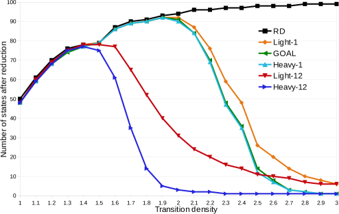
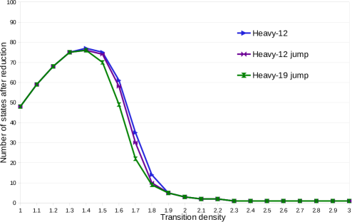
Figure 13. We consider Tabakov-Vardi Büchi automata with $n=100$, $|\Sigma|=2$, ${\it ad}=0.5$ and the range of ${\it td}=1.0,1.1,\dots,3.0$. Each curve represents a different method, and we plot the number of states after reduction. Each data point is the average of $300$ random automata.

Figure 14. Moreover, we plotted the effects of two methods that augment our Heavy reduction algorithm by quotienting with (a variant of) the jumping-safe preorders of [16, 17]: Heavy-12 jump and Heavy-19 jump. These yield another slight improvement in reduction, but are slower to compute.

The inherent difficulty of the reduction problem, and thus also the effectiveness of reduction methods, depends strongly on the class of random automata, i.e., on the parameters listed above. Thus, one needs to compare the methods over the whole range, not just for one example. Variations in the acceptance density ${\it ad}$ do not affect Heavy-k much, but very small values make reduction harder for the other methods. By far the most important parameter is the transition density ${\it td}$, and thus we compare different techniques across different values of ${\it td}$. Fig. 14 and 14 compare the effect of different techniques. Each curve represents a different method: RD (just remove dead states), Light-1, Light-12, Heavy-1, Heavy-12, and GOAL. The GOAL curve shows the best effort of all previous techniques (as implemented in GOAL), which include RD, quotienting with backward and forward simulation, pruning of little brother transitions and the fair simulation reduction of [35].

Sparse automata with low ${\it td}$ have more dead states. Thus the RD method achieves a certain reduction at low ${\it td}$, but this effect vanishes as ${\it td}$ gets higher. For ${\it td}\leq 1.4$ the effect of RD dominates. In that range, the other techniques have only a very small effect. In the range $1.5\leq{\it td}\leq 2.0$, GOAL still has hardly any effect (apart from that of RD), but Light-12 and Heavy-12 achieve a significant reduction. For ${\it td}\geq 2.0$, GOAL begins to have an effect, but it is much smaller than that of our best techniques.

Generally, GOAL reduces just slightly worse than Heavy-1, but it is no match for our best techniques like Heavy-12. Heavy-12 vastly outperforms all other previous techniques, particularly in the interesting range between ${\it td}=1.4$ and ${\it td}=2.5$. Moreover, the reduction of GOAL (in particular the fair simulation reduction of [35]) is very slow. For GOAL, the average reduction time per automaton varies between 39s (at ${\it td}=1.0$) and 612s (maximal at ${\it td}=2.9$). In contrast, for Heavy-12, the average reduction time per automaton varies between 0.012s (at ${\it td}=1.0$) and 1.482s (max. at ${\it td}=1.7$). So Heavy-12 reduces not only much better, but also at least $400$ times faster than GOAL (see also the scalability tests below).

The computation time of Heavy-k depends both on the density ${\it td}$ and on the lookahead $k$. Fig. 15 shows the average computation time of Heavy-k on automata with $100$ states, ${\it ad}=0.5$, $|\Sigma|=2$ and varying transition density ${\it td}$ and lookahead $k$. The most difficult cases are those where size reduction is possible (and thus the algorithm does not give up quickly), but where the size of the instance is not massively reduced. (If some step in the algorithm greatly reduced the size of an instance, then subsequent computations on the now smaller automaton would be much faster.) For Heavy-k, the peak of the average computation time is around ${\it td}=1.6,1.7$ (like in the scalability test; see below).

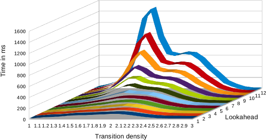
Figure 15. Average computation time for reduction with Heavy-k on Tabakov-Vardi random Büchi automata with $n=100$ states, $|\Sigma|=2$, ${\it ad}=0.5$ and varying transition density ${\it td}$ and lookahead $k$.

For ${\it td}\geq 2.0$, Heavy-12 yields very small automata. Many of these are even universal, i.e., with just one state and a universal loop. However, this frequent universality is not due to trivial reasons (otherwise simpler techniques like Light-1 and GOAL would also recognize this). For example, we argue that in the tested interval of parameters $n$, $|\Sigma|$ and ${\it td}$, there are not sufficiently many transitions to alone explain that the automaton is universal—and thus there are more interesting non-local structural reasons which make the automata universal. Given Tabakov-Vardi random automata with parameters $n$, $|\Sigma|$ and ${\it td}$, let $U(n,|\Sigma|,{\it td})$ be the probability that every state has at least one outgoing transition for every symbol in $\Sigma$. Such an automaton would be trivially universal if ${\it ad}=1$. (Note that ${n\choose k}=0$ for $k>n$.)

Theorem 9.1.

We have $U(n,|\Sigma|,{\it td})=(\alpha(n,T)/\beta(n,T))^{|\Sigma|}$, where $T=\lfloor n\cdot{\it td}\rfloor$, $\beta(n,T)={{n^{2}}\choose T}$, and $\alpha(n,T)=\sum_{m=n}^{n^{2}}{{m-n}\choose{T-n}}\sum_{i=0}^{n}(-1)^{i}{n\choose i}{{m-in-1}\choose{n-1}}$.

Proof.

For each symbol in $\Sigma$ there are $T=\lfloor n\cdot{\it td}\rfloor$ transitions and $n^{2}$ possible places for transitions, described as a grid. $\alpha(n,T)$ is the number of ways $T$ items can be placed onto an $n\times n$ grid s.t. every row contains $\geq 1$ item, i.e., every state has an outgoing transition. $\beta(n,T)$ is the number of possibilities without this restriction, which is trivially ${{n^{2}}\choose T}$. Since the Tabakov-Vardi model chooses transitions for different symbols independently, we have $U(n,|\Sigma|,{\it td})=(\alpha(n,T)/\beta(n,T))^{|\Sigma|}$. It remains to compute $\alpha(n,T)$. For the $i$-th row let $x_{i}\in\{1,\dots,n\}$ be the maximal column containing an item. The remaining $T-n$ items can only be distributed to lower columns. Thus $\alpha(n,T)=\sum_{x_{1},\dots,x_{n}}{{(\sum x_{i})-n}\choose{T-n}}$. With $m=\sum x_{i}$ and a standard dice-sum problem [58] the result follows. ∎

For $n=100$, $|\Sigma|=2$ we obtain the following values for $U(n,|\Sigma|,{\it td})$: $10^{-15}$ for ${\it td}=2.0$, $2.9\cdot 10^{-5}$ for ${\it td}=3.0$, $0.03$ for ${\it td}=4.0$, $0.3$ for ${\it td}=5.0$, $0.67$ for ${\it td}=6.0$, and $0.95$ for ${\it td}=8.0$. So this transition saturation effect is negligible in our tested range with ${\it td}\leq 3.0$.

While Heavy-12 performs very well, an even smaller lookahead can already be sufficient for a good reduction. However, this depends very much on the density ${\it td}$ of the automata. Fig. 16 shows the effect of the lookahead by comparing Heavy-k for varying $k$ on different classes of random automata with different density.

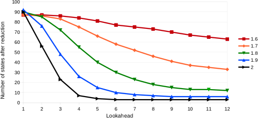
Figure 16. The effect of the lookahead on Tabakov-Vardi automata. We set $n=100$, $|\Sigma|=2$, and ${\it ad}=0.5$, and vary the transition density ${\it td}=1.6,1.7,1.8,1.9,2.0$ and the lookahead from $1,\dots,12$. Every point is the average of the Heavy-k minimization of $1000$ random automata. While a lower lookahead suffices for denser automata, more is needed for sparser instances.

9.1.2. Density of simulations on NBA

The big advantage of Heavy-12 over Light-12 is due to the pruning techniques. However, these only reach their full potential at higher lookaheads (thus the smaller difference between Heavy-1 and Light-1). Indeed, the simulation relations get much denser with higher lookahead $k$, as Fig. 17 shows.

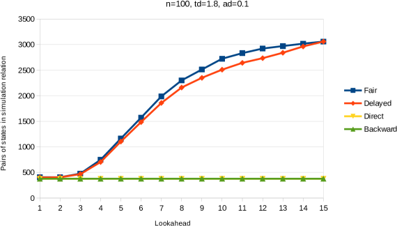
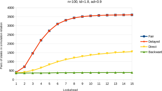
Figure 17. We consider Tabakov-Vardi random Büchi automata with $n=100$, $|\Sigma|=2$ and ${\it td}=1.8$ (a non-trivial case; larger ${\it td}$ yield larger simulations). We let ${\it ad}=0.1$ (resp. ${\it ad}=0.9$), and plot the size of fair, delayed, direct, and backward $k$-lookahead simulation as $k$ increases from $1$ to $15$. Every point is the average of $1000$ automata.

Fair and delayed simulation relations are not much larger than direct simulation for $k=1$, but they benefit strongly from higher $k$. Backward simulation increases only slightly (e.g., from $363$ pairs for lookahead $1$ to $397$ pairs for lookahead $15$ in the case of ${\it ad}=0.9$). Initially, it seems as if backward (resp. direct) simulation does not benefit from higher $k$ if ${\it ad}$ is small (on random automata), but this is wrong. Even random automata get less random during the Heavy-k reduction process, making lookahead more effective for backward (resp. direct) simulation. Consider the case of $n=300$, ${\it td}=1.8$ and ${\it ad}=0.1$. Initially, the average ratio $|\preceq^{{12}\textrm{-}\mathsf{di}}|/|\preceq^{{1}\textrm{-}\mathsf{di}}|$ is $1.00036$, but after quotienting with $\preceq^{{12}\textrm{-}\mathsf{de}}$ this ratio is $1.103$.

9.1.3. Sparseness of the reduced NBA

The number of states of a nondeterministic automaton is not the only measure of its complexity. The amount of nondeterministic branching is also highly relevant in many applications, e.g., in model checking [63], as well as the actual position of accepting states when one analyzes the behavior of specific emptiness checking algorithms [10]. Automata with a high transition density (i.e., a large number of transitions, relative to the number of states and symbols) have more nondeterministic branching. Conversely, automata with a low transition density have less nondeterministic branching. We call the latter type sparse automata. A priori, a method that reduces the number of states of automata might influence its transition density in either direction. In particular, the density might become higher—e.g., there might be a tradeoff to describe the same language with fewer states but more transitions (per state). However, we show in Fig. 18 that our Heavy-12 reduction method does not incur this tradeoff. Indeed, it yields automata that are not only smaller, but also sparser.

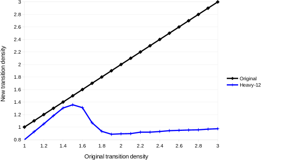
Figure 18. Heavy-12 produces sparse automata. We consider Tabakov-Vardi random Büchi automata with $n=100$, $|\Sigma|=2$, ${\it ad}=0.5$ and ${\it td}=1.0,\dots,3.0$. The x-axis is the transition density of the original automata while the y-axis is the average density of the reduced automata. The two curves show the average transition density of the original automata (this is just the identity function) and the average transition density of the Heavy-12 reduced automata. Every point is the average of $1000$ automata.

9.1.4. Reducing NBA derived from LTL

For model checking [40], LTL-formulae are converted into Büchi automata. This conversion has been extensively studied and there are many different algorithms which try to construct the smallest possible automaton for a given formula; cf. references in [68] and [9] and [1].

It should be noted however, that LTL is designed for human readability and does not cover the full class of $\omega$-regular languages. Moreover, the website and database Büchi Store [69, 70] contains handcrafted automata for almost every human-readable LTL-formula, and almost all of these automata have $\leq 10$ states.

Moreover, new LTL to Büchi automata converters are being developed every year [68, 9, 1], and it is not in the scope of this paper to benchmark all converters.

For the scope of this paper, Büchi automata generated from random LTL formulae are simply yet another class of test cases for our size reduction algorithm. In particular, they are different from the Tabakov-Vardi random automata.

In order to get interesting test cases, we used random LTL formulae that are larger than typical human-readable ones and obtained larger automata on average (see below).

Moreover, for LTL model checking, the size of the automata is not the only criterion [63], since more nondeterminism also makes the problem harder. However, our transition pruning techniques reduce the amount of nondeterministic branching, and yield automata that are not only smaller but also sparser (i.e., ‘less nondeterministic’); cf. our results below, and also Sec. 9.1.3.

Using a function of GOAL, we created 300 random LTL-formulae of non-trivial size: length 70, 4 predicates and probability weights 1 for boolean and 2 for future operators. We then converted these formulae to Büchi automata and reduced them with GOAL. Of the 14 different converters implemented in GOAL we chose LTL2BA [33] (as implemented in GOAL, which behaves slightly differently from the stand-alone LTL2BA tool) since it was the only one (in GOAL) which could handle such large formulae. (The second best was COUVREUR [21] which succeeded on 90% of the instances, but produced much larger automata than LTL2BA. The other converters ran out of time (4h) or memory (14GB) on most instances.) We thus obtained 300 automata and reduced them with GOAL. The resulting automata vary significantly in size from 1 state to 1722 states.

Then we tested how much further these automata could be reduced in size by our Heavy-12 method. In summary, 82% of the automata could be further reduced in size. The average number of states declined from 138 to 78, and the average number of transitions from 3102 to 1270. Since larger automata have a disproportionate effect on averages, we also computed the average reduction ratio per automaton, i.e., $(1/300)\sum_{i=1}^{300}{\it newsize}_{i}/{\it oldsize}_{i}$. (Note the difference between the average ratio and the ratio of averages.) The average ratio was $0.76$ for states and $0.68$ for transitions. The computation times for reduction vary a lot due to different automata sizes (average 4.1s), but were always less than the time used by the LTL to automata translation. If one only considers the 150 automata above median size (30 states) then the results are even stronger. 100% of these automata could be further reduced in size. The average number of states declined from 267 to 149, and the average number of transitions from 6068 to 2435. The average reduction ratio was $0.65$ for states and $0.54$ for transitions.

9.1.5. Reducing NBA derived from mutual exclusion protocols

In Table 3 we consider automata derived from mutual exclusion protocols. The protocols were described in a language of guarded commands and automatically translated into Büchi automata, whose size is given in the column ‘Original’. We reduce these automata with GOAL and with our Heavy-12 method and describe the sizes of the resulting automata and the runtime in subsequent columns.

Automaton name	Original		GOAL		Time	Heavy-12		Time
	Trans.	States	Tr.	St.	GOAL	Tr.	St.	Heavy-12
bakery.1.c.ba	2597	1506	N/A	N/A	$>2h$	696	477	5.3s
bakery.2.c.ba	2085	1146	N/A	N/A	$>2h$	927	643	7.6s
fischer.3.1.c.ba	1401	638	14	10	15.38s	14	10	0.86s
fischer.3.2.c.ba	3856	1536	212	140	4529s	96	70	3.4
fischer.2.c.ba	67590	21733	N/A	N/A	oom(14GB)	316	192	253.5s
phils.1.1.c.ba	464	161	362	134	540.3s	359	134	1.5s
phils.2.c.ba	2350	581	284	100	164.2s	225	97	1.8s
mcs.1.2.c.ba	21509	7968	108	69	2606.7s	95	62	42.9s

Table 3. Reduction of NBA derived from mutual exclusion protocols, comparing GOAL [68] (version 2012-05-02 on Java 6) and RABIT/Reduce method Heavy-12 (version 2.4.0 on Java 7) using an Intel i7-740, 1.73 GHz. In some instances GOAL ran out of time (2h) or memory (14GB).

9.1.6. Scalability of NBA reduction

We tested the scalability of Heavy-12 reduction by applying it to Tabakov-Vardi random automata of increasing size $n$ but fixed ${\it td}$, ${\it ad}$ and $\Sigma$. We ran four separate tests with ${\it td}=1.4,1.6,1.8$ and $2.0$. In each test we fixed ${\it ad}=0.5$, $|\Sigma|=2$ and increased the number of states from $n=50$ to $n=1000$ in increments of 50. For each parameter point we created $300$ random automata and reduced them with Heavy-12. We analyze the average size of the reduced automata in percent of the original size $n$, and how the average computation time increases with $n$.

For ${\it td}=1.4$ the average size of the reduced automata stays around $77\%$ of the original size, regardless of $n$. For ${\it td}=1.6$ it stays around $65\%$. For ${\it td}=1.8$ it decreases from $28\%$ at $n=50$ to $2\%$ at $n=1000$. For ${\it td}=2.0$ it decreases from $8\%$ at $n=50$ to $<1\%$ at $n=1000$. See Fig. 19.

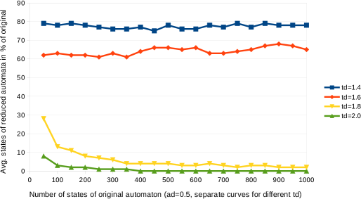
Figure 19. Reduction of Tabakov-Vardi random Büchi automata with ${\it ad}=0.5$, $|\Sigma|=2$, and increasing $n=50,100,\dots,1000$. Different curves for different ${\it td}$. We plot the average size of the Heavy-12 reduced automata, in percent of their original size. Every data point is the average of $300$ automata.

Note that the lookahead of 12 did not change with $n$. Surprisingly, larger automata do not require larger lookahead for a good reduction.

In Fig. 20 we plot the average computation time (measured in ms) in $n$ and then compute the optimal fit of the function ${\it time}=a\cdot n^{b}$ to the data by the least-squares method, i.e., this computes the parameters $a$ and $b$ of the function that most closely fits the experimental data. The important parameter is the exponent $b$. For ${\it td}=1.4,1.6,1.8,2.0$ we obtain $0.0036\cdot n^{2.26}$, $0.012\cdot n^{2.41}$, $0.02\cdot n^{2.16}$ and $0.0046\cdot n^{2.37}$, respectively. We also measured the median time used for reduction, and it was always very close to the average time.

Thus, the average-case complexity of Heavy-12 scales slightly above quadratically (with exponents between $2.16$ and $2.41$). This is especially surprising given that Heavy-12 does not only compute one simulation relation but potentially many simulations until the repeated reduction reaches a fixpoint. Quadratic complexity is the very best one can hope for in any method that explicitly compares states/transitions by simulation relations, since the relations themselves are of quadratic size. Lower complexity is only possible with pure partition refinement techniques (e.g., bisimulation, which is $O(n\log n)$ for graphs with a fixed out-degree), but these achieve even less reduction than quotienting with direct simulation (i.e., almost nothing on hard instances).

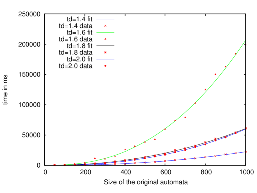
Figure 20. Average computation time for Heavy-12 on Tabakov-Vardi Büchi automata with ${\it ad}=0.5$, $|\Sigma|=2$ and ${\it td}=1.4,1.6,1.8,2.0$, with a least squares fit of the function $y=a\cdot x^{b}$. The x-axis shows the number of states of the original automata and the y-axis shows the average runtime in ms. Each data point is the average of 300 automata.

9.1.7. Language inclusion testing for NBA

We evaluated the language inclusion testing algorithm of Sec. 8.3 (with lookahead up-to $15$) on non-trivial instances and compared its performance to previous techniques like ordinary fair simulation checking and the best effort of GOAL (which uses simulation-based reduction followed by checking fair simulation preorder and an on-the-fly variant of Piterman’s construction [60, 68]).

We considered pairs of Tabakov-Vardi random automata with $1000$ states each, $|\Sigma|=2$ and ${\it ad}=0.5$. For each separate case of ${\it td}=1.6,1.8$ and $2.0$, we created $300$ such automata pairs and tested if language inclusion holds. (For ${\it td}<1.6$ inclusion rarely holds, except trivially if one automaton has the empty language. For ${\it td}>2$ inclusion holds very often and is relatively easy to prove, since the languages of the automata are often almost universal.)

For ${\it td}=1.6$ our algorithm solved $297$ of $300$ instances (i.e., 99%): $45$ included, $252$ not included, and $3$ timeouts (30min). Of the $45$ included cases, $16$ were shown during the reduction/preprocessing (step 1), $29$ were shown by jumping fair simulation, using lookaheads between 9 and 15 (step 2), and none of the included cases were shown by the Ramsey method (step 4). (Step 3 can only prove non-inclusion.) The average computation time for the included cases was $192.6$ seconds. Of the $252$ non-included cases, most were shown very quickly by short counterexamples. The average computation time for the non-included cases was $33$ seconds. In contrast, ordinary fair simulation solved only $13$ included instances. GOAL (timeout 30min, 14GB memory) solved only $13$ included instances (the same $13$ as fair simulation) and $155$ non-included instances, i.e., a success rate of just 56%. (The results were the same if the timeout for GOAL was increased to 60min.)

For ${\it td}=1.8$ our algorithm solved $300$ of $300$ instances (i.e., 100%): $103$ included, and $197$ non-included. Of the $103$ included cases, all were shown during reduction/preprocessing (step 1), and none by steps 2, 3, 4. The average computation time for the included cases was $118$ seconds. The average computation time for the $197$ non-included cases was $6.6$ seconds. Ordinary fair simulation solved only 5 included instances. GOAL (timeout 30min, 14GB memory) solved only 5 included instances (the same 5 as fair simulation) and $115$ non-included instances, i.e., a success rate of just 40%.

For ${\it td}=2.0$ our algorithm solved $300$ of $300$ instances (i.e., 100%): $143$ included, and $157$ non-included. Of the $143$ included cases, all were shown during reduction/preprocessing (step 1) and none by steps 2, 3, 4. The average computation time for the included cases was $127$ seconds. The average computation time for the $157$ non-included cases was $5.4$ seconds. Ordinary fair simulation solved only 1 of the $143$ included instances. GOAL (timeout 30min, 14GB memory) solved only 1 of $143$ included instances (the same one as fair simulation) and $106$ of $157$ non-included instances, i.e., a success rate of just 35.7%.

9.2. Finite automata

9.2.1. Reduction of random NFA

Like in Sec. 9.1.1, we consider Tabakov-Vardi random automata. However, here we interpret these automata as NFA instead of Büchi automata, and reduce them such that the finite-word language is preserved.

Generally, random NFA are harder to reduce in size than random NBA, because for NFA it matters when (i.e., in exactly which step) one encounters an accepting state. In contrast, for NBA it only matters whether one encounters accepting states infinitely often. Thus random NFA have somewhat more complex languages than random NBA to begin with.

The generated Tabakov-Vardi random automata normally have many accepting states. However, before applying the reduction methods, we first transform the NFA into equivalent ones with just a single accepting state without any outgoing transitions. (Unless the empty word is in the language, in which case the initial state is accepting too.) Note that the same cannot be done for Büchi automata. This transformation of NFA makes direct (and backward) simulations significantly larger, and thus increases the effect of the reduction methods. The reason is that direct/backward simulations need to match accepting states immediately, regardless of whether the input word has already been fully read to the end or not. This makes it very hard for Duplicator to win the simulation game, and thus yields very small direct/backward simulations. However, if an NFA has just a single accepting state without any outgoing transitions then this state needs to be matched at most once in a simulation game, which is much easier. Note that this transformation does not actually make an NFA more complex, in the following sense. While one gets some additional transitions (albeit of a special type, all going to the one accepting state), the description of the set of accepting states becomes correspondingly simpler, since it just consists of a single element. Fig. 21 shows that doing this transformation is very important. Without it, even the best methods, like Heavy-12, perform very poorly (see the graph for Heavy-12, multi acc states). For random NFA with transition density $\leq 1.5$, all methods do not achieve much more than remove dead states. For such automata, the transformation into the form with one accepting state does not make much difference, except for the tradeoff between the number of transitions and the complexity of describing the set of accepting states. (See also the results on the transition density in Fig. 24.)

Fig. 22 shows the effect of different reduction methods (that all use the trick of transforming NFA into a form with a single accepting state). Like for Büchi automata, our Heavy method reduces the size far more than any simpler technique.

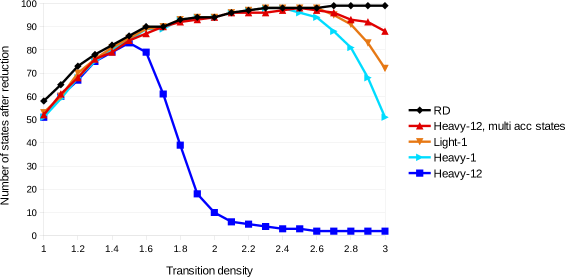
Figure 21. Tabakov-Vardi random NFA with $n=100$, $|\Sigma|=2$, ${\it ad}=0.5$ and the range of ${\it td}=1.0,1.1,\dots,3.0$. Each curve represents a different reduction method: RD (just remove dead states). Heavy-12, multi acc states: Like Heavy-12 but without the transformation into a form with a single accepting state. Light-1, Heavy-1 and Heavy-12 all use the transformation into a form with a single accepting state. Each data point is the average of $1000$ random automata.

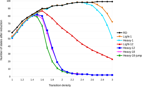
Figure 22. Tabakov-Vardi random NFA with $n=100$, $|\Sigma|=2$, ${\it ad}=0.5$ and the range of ${\it td}=1.0,1.1,\dots,3.0$. Each curve represents a different reduction method: RD (just remove dead states), Light-1, Heavy-1, Light-12, Heavy-12, Heavy-18 and Heavy-18 jump (which is Heavy-18 augmented by quotienting with (a variant of) the jumping-safe preorders of [16, 17]). Each data point is the average of $1000$ random automata.

9.2.2. Density of simulations on NFA

In Fig. 23 we measure the density of direct simulation and backward simulation on Tabakov-Vardi random NFA. We take $n=100$, $|\Sigma|=2$ and ${\it td}=1.8$ (a non-trivial case; larger ${\it td}$ yield larger simulations). To show the effect of the acceptance density, we consider two cases: ${\it ad}=0.1$ and ${\it ad}=0.9$. Like in Sec. 9.2.1, these NFA had been transformed into equivalent ones with just a single accepting state. This makes direct simulation on NFA significantly larger than on Büchi automata, particularly if ${\it ad}$ is high. We plot the size of direct and backward simulation as the lookahead $k$ increases from $1$ to $15$.

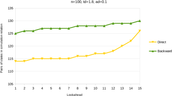
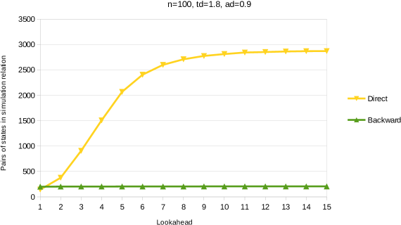
Figure 23. Density of direct simulation and backward simulation on Tabakov-Vardi random NFA with $n=100$, $|\Sigma|=2$, ${\it td}=1.8$ and ${\it ad}=0.1$ (top) and ${\it ad}=0.9$ (bottom), respectively. On the x-axis, the lookahead increases from $1$ to $15$. On the y-axis, we measure the size of the simulation relations. Every data point is the average of $1000$ random automata.

9.2.3. Sparseness of reduced NFA

Like for Büchi automata in Sec. 9.1.3, we measure the average transition density of the Heavy-12 reduced random NFA. Our algorithm first transforms the NFA into a form with only one accepting state. This adds a significant number of transitions and thus increases the transition density. However, for NFA with transition density $>1.5$, the Heavy-12 procedure then decreases the transition density again. In Fig. 24 we thus plot the original transition density, the density after the transformation into the form with one accepting state and the density of the Heavy-12 reduced automata.

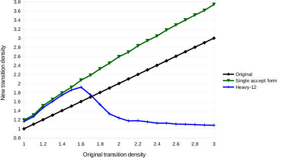
Figure 24. Heavy-12 produces sparse automata. We consider Tabakov-Vardi random NFA with $n=100$, $|\Sigma|=2$, ${\it ad}=0.5$ and ${\it td}=1.0,\dots,3.0$. The x-axis is the transition density of the original automata while the y-axis is the average density of the new automata. The three curves show the average transition density of the original automata (this is just the identity function), the density after the transformation into the form with one accepting state, and the average transition density of the Heavy-12 reduced automata. Every point is the average of $1000$ automata.

9.2.4. Scalability of NFA reduction

We test the scalability of reducing NFA with Heavy-12 by testing Tabakov-Vardi random automata of increasing size $n$ but fixed ${\it td}$, ${\it ad}$ and $\Sigma$. We ran four separate tests with ${\it td}=1.4,1.6,1.8$ and $2.0$. In each test we fixed ${\it ad}=0.5$, $|\Sigma|=2$ and increased the number of states from $n=50$ to $n=600$ in increments of $50$. For each parameter point we created $300$ random automata and reduced them with Heavy-12. We analyze the average size of the reduced automata in percent of the original size $n$, and how the average computation time increases with $n$.

For ${\it td}=1.4$ the average size of the reduced automata stays around $77\%$ of the original size, regardless of $n$. For ${\it td}=1.6$ it stays around $81\%$. For ${\it td}=1.8$ it decreases from $53\%$ at $n=50$ to $9\%$ at $n=600$. For ${\it td}=2.0$ it decreases from $23\%$ at $n=50$ to $1\%$ at $n=600$. See Fig. 25.

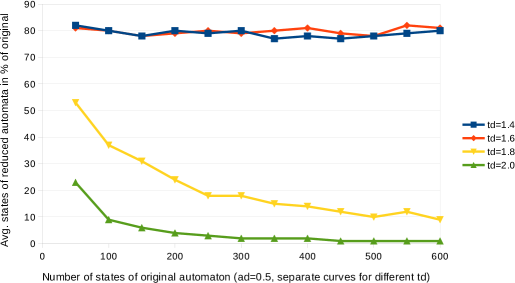
Figure 25. Reduction of Tabakov-Vardi random NFA with ${\it ad}=0.5$, $|\Sigma|=2$, and increasing $n=50,100,\dots,600$. Different curves for different ${\it td}$. We plot the average size of the Heavy-12 reduced automata, in percent of their original size. Every data point is the average of $300$ automata.

Note that the lookahead of 12 did not change with $n$. Surprisingly, larger automata do not require larger lookahead for a good reduction.

Unlike in Büchi automata reduction, the average time to reduce NFA was much higher than the median time (for transition densities $1.6$ and $1.8$). For example, the average time to reduce a random NFA with $600$ states and ${\it td}=1.6$ was 199s, while the median time was 43s. For ${\it td}=1.8$ the average and median times were 1316s and 20s, respectively. Apparently, a few random NFA are very hard instances which increase the average reduction time. Therefore, we analyze both the average and the median reduction time for NFA below.

In Fig. 26, we plot the median computation time (measured in ms) in $n$ and then compute the optimal fit of the function ${\it time}=a\cdot n^{b}$ to the data by the least-squares method as above. For ${\it td}=1.4,1.6,1.8,2.0$ we obtain $0.0058\cdot n^{2.22}$, $0.011\cdot n^{2.37}$, $0.0048\cdot n^{2.38}$ and $0.0048\cdot n^{2.26}$, respectively. So the median computation times scale slightly above quadratically.

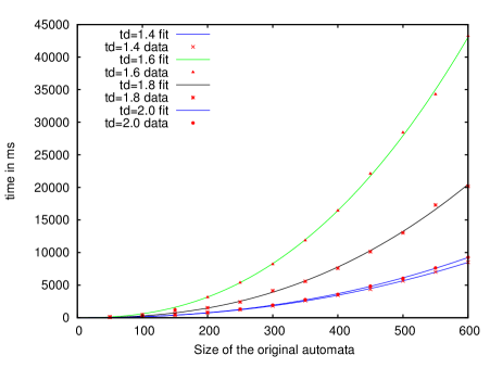
Figure 26. Median computation time for Heavy-12 on Tabakov-Vardi NFA with ${\it ad}=0.5$, $|\Sigma|=2$ and ${\it td}=1.4,1.6,1.8,2.0$, with a least squares fit of the function $y=a\cdot x^{b}$. The x-axis shows the number of states of the original automata and the y-axis shows the median runtime in ms.

In Fig. 28 we plot the average computation time (measured in ms) in $n$ and then compute the optimal fit of the function ${\it time}=a\cdot n^{b}$ to the data by the least-squares method, i.e., this computes the parameters $a$ and $b$ of the function that most closely fits the experimental data. The important parameter is the exponent $b$. For ${\it td}=1.4,1.6,1.8,2.0$ we obtain $0.0033\cdot n^{2.33}$, $1.15\cdot 10^{-4}\cdot n^{3.33}$, $3\cdot 10^{-27}\cdot n^{11.7}$ and $0.008\cdot n^{2.20}$, respectively. Clearly, for ${\it td}=1.8$, the curve fits the experimental data extremely poorly (with exponent $b=11.7$ and scale factor $a=3\cdot 10^{-27}$). Apparently, for ${\it td}=1.8$, a few very hard instances create outliers that distort the averages (unlike the median). In Fig. 27 (resp. Fig. 28) we plot the averages including (resp. excluding) the case of ${\it td}=1.8$.

Figure 27. Average computation time for Heavy-12 on Tabakov-Vardi NFA with ${\it ad}=0.5$, $|\Sigma|=2$ and ${\it td}=1.4,1.6,1.8,2.0$, with a least squares fit of the function $y=a\cdot x^{b}$. The x-axis shows the number of states of the original automata and the y-axis shows the average runtime in ms. Note the poor fit of the curve for ${\it td}=1.8$.

Figure 28. Average computation time for Heavy-12 on Tabakov-Vardi NFA with ${\it ad}=0.5$, $|\Sigma|=2$ and ${\it td}=1.4,1.6,2.0$, with a least squares fit of the function $y=a\cdot x^{b}$. The x-axis shows the number of states of the original automata and the y-axis shows the average runtime in ms.

10. Extensions: Adding Transitions

In this section we describe a technique, called saturation, that reduces the number of states of automata by adding more transitions. The idea is that certain transitions may be added to an automaton without changing its language when other better transitions are already present. Conceptually, this is dual to the transition pruning techniques of Sec. 5. This technique is implemented in our tool [15] and can have a significant effect on some instances. However, it is not part of the default Heavy-k algorithm (described and tested in Sections 7 and 9), due to low efficiency and a tradeoff between the numbers of states and transitions. Note that adding transitions itself does not change the number of states. However, the changed automaton might allow the application of further quotienting that then reduces the number of states. Moreover, the changed automaton might be treated with the pruning techniques from Sec. 5, and this might remove some transitions other than the recently added ones. This modification might pave the way for further quotienting, etc., which finally results in an automaton with fewer states, and possibly even fewer transitions, than the one produced by the default Heavy-k method.

One downside is that, even if the number of states eventually decreases, not all the added transitions can be removed again. So one might obtain an automaton with fewer states but more transitions than the one produced by Heavy-k. This tradeoff effect between the numbers of states and transitions exists in practice, though it is not very strong; see the experiments in Sec. 10.3.

Definition 10.1.

Let $\mathcal{A}=(\Sigma,Q,I,F,\delta)$ be an automaton, $\Delta=Q\times\Sigma\times Q$ the set of all possible transitions between states in $\mathcal{A}$, $S\subseteq\Delta\times\Delta$ a reflexive binary relation on $\Delta$, and, for a set of transitions $\Gamma\subseteq\Delta$,

$$S^{-1}(\Gamma)=\{(p^{\prime},\sigma^{\prime},r^{\prime})\in\Delta\;|\;\exists(p,\sigma,r)\in\Gamma\cdot(p^{\prime},\sigma^{\prime},r^{\prime})\;S\;(p,\sigma,r)\}.$$

The $S$-saturated automaton is defined as ${\it Sat}({\mathcal{A}},{S})\;\coloneqq\;(\Sigma,Q,I,F,\delta^{\prime})$, where $\delta^{\prime}=S^{-1}(\delta)$.

The intuition is that more transitions can be added without changing the language if better (i.e., $S$-larger) transitions already exist. Since $S$ is reflexive, saturation only adds transitions, and thus $\mathcal{A}\subseteq{\it Sat}({\mathcal{A}},{S})$. When the converse inclusion also holds, we say that $S$ is good for saturation.

Definition 10.2.

A relation $S\subseteq\Delta\times\Delta$ is good for saturation (GFS) if ${\it Sat}({\mathcal{A}},{S})\approx\mathcal{A}$.

The GFS property is downward closed in the space of reflexive relations, i.e., if $S$ is GFS and ${\it id}\subseteq S^{\prime}\subseteq S$, then $S^{\prime}$ is also GFS.

We study GFS relations which add transitions to already existing states, and they do so by comparing the endpoints of such transitions over the same input symbol. (This is similar to our pruning technique from Sec. 5.) Formally, given two binary state relations $\mathrel{R_{b}},\mathrel{R_{\!f}}\subseteq Q\times Q$ for the source and target endpoints, respectively, we define

$$\mathrel{S({\mathrel{R_{b}}},{\mathrel{R_{\!f}}})}=\{((p,\sigma,r),(p^{\prime},\sigma,r^{\prime}))\in\Delta\times\Delta\;|\;p\mathrel{\mathrel{R_{b}}}p^{\prime}\textrm{ and }r\mathrel{\mathrel{R_{\!f}}}r^{\prime}\}.$$

$\mathrel{S({\cdot},{\cdot})}$ is monotone in both arguments.

Given an automaton $\mathcal{A}$ and relations $\mathrel{R_{b}},\mathrel{R_{\!f}}$ on the states of $\mathcal{A}$, we will construct a new automaton $\mathcal{B}={\it Sat}({\mathcal{A}},{\mathrel{S({\mathrel{R_{b}}},{\mathrel{R_{\!f}}})}})$. When reasoning about whether $\mathrel{S({\mathrel{R_{b}}},{\mathrel{R_{\!f}}})}$ is GFS (i.e., whether $\mathcal{B}\approx\mathcal{A}$), it is important to keep in mind that the relations $\mathrel{R_{b}},\mathrel{R_{\!f}}$ are valid only w.r.t. $\mathcal{A}$, but not necessarily w.r.t. $\mathcal{B}$.

10.1. Saturation of NBA

$\mathrel{R_{b}}\backslash\mathrel{R_{\!f}}$	${\it id}$	$\sqsubseteq^{\mathsf{di}}$	$\subseteq^{\mathsf{di}}$	$\sqsubseteq^{\mathsf{fx\textrm{-}de}}$	$\subseteq^{\mathsf{de}}$	$\sqsubseteq^{\mathsf{f}}$	$\sqsupseteq^{\mathsf{bw\textrm{-}di}}$	$\supseteq^{\mathsf{bw\textrm{-}di}}$
${\it id}$	$\checkmark$	$\checkmark$	$\checkmark$	$\checkmark$	$\times$	$\times$	$\checkmark$	$\checkmark$
$\sqsupseteq^{\mathsf{di}}$	$\checkmark$	$\checkmark$	$\checkmark$	$\checkmark$	$\times$	$\times$	$\times$	$\times$
$\supseteq^{\mathsf{di}}$	$\checkmark$	$\checkmark$	$\checkmark$	$\checkmark$	$\times$	$\times$	$\times$	$\times$
$\sqsupseteq^{\mathsf{fx\textrm{-}de}}$	$\checkmark$	$\checkmark$	$\checkmark$	$\checkmark$	$\times$	$\times$	$\times$	$\times$
$\supseteq^{\mathsf{de}}$	$\times$	$\times$	$\times$	$\times$	$\times$	$\times$	$\times$	$\times$
$\sqsupseteq^{\mathsf{f}}$	$\times$	$\times$	$\times$	$\times$	$\times$	$\times$	$\times$	$\times$
$\sqsubseteq^{\mathsf{bw\textrm{-}di}}$	$\checkmark$	$\times$	$\times$	$\times$	$\times$	$\times$	$\checkmark$	$\checkmark$
$\subseteq^{\mathsf{bw\textrm{-}di}}$	$\checkmark$	$\times$	$\times$	$\times$	$\times$	$\times$	$\checkmark$	$\checkmark$

Table 4. GFS relations $\mathrel{P({\mathrel{R_{b}}},{\mathrel{R_{\!f}}})}$ for NBA. $\checkmark$ denotes yes and $\times$ denotes no.

We study which semantic preorders induce GFS relations on NBA. Our results are summarized in Table 4.

In the transition pruning techniques of Sec. 5, the source states of transitions were compared w.r.t. backward simulation (resp. trace inclusion), while the target states were compared w.r.t. (various types of) forward simulation (resp. trace inclusion). However, for saturation this would be incorrect as the counterexample from Fig. 29 shows. In this automaton $\mathcal{A}$ (without the dashed transition) we have that $(r,a,r)\mathrel{S({\sqsubseteq^{\mathsf{bw\textrm{-}di}}},{\sqsubseteq^{\mathsf{di}}})}(p,a,q)$, but adding the dashed transition $(r,a,r)$ changes the language, since $a^{\omega}$ is now accepted, i.e., $a^{\omega}\in\mathcal{L}({\it Sat}({\mathcal{A}},{\mathrel{S({\sqsubseteq^{\mathsf{bw\textrm{-}di}}},{\sqsubseteq^{\mathsf{di}}})}}))\setminus\mathcal{L}(\mathcal{A})$. Thus, $\mathrel{S({\sqsubseteq^{\mathsf{bw\textrm{-}di}}},{\sqsubseteq^{\mathsf{di}}})}$ is not GFS. A similar example in Fig. 30 shows that $\mathrel{S({\sqsupseteq^{\mathsf{di}}},{\sqsupseteq^{\mathsf{bw\textrm{-}di}}})}$ is not GFS either: Here $(p,a,q)\mathrel{S({\sqsupseteq^{\mathsf{di}}},{\sqsupseteq^{\mathsf{bw\textrm{-}di}}})}(r,a,s)$, and thus the dashed transition $p\stackrel{{\scriptstyle a}}{{\longrightarrow}}q$ is added, which causes the new word $a^{\omega}$ to be accepted—while this was not the case in the original automaton. While $\mathrel{S({\sqsubseteq^{\mathsf{bw\textrm{-}di}}},{\sqsubseteq^{\mathsf{di}}})}$ and $\mathrel{S({\sqsupseteq^{\mathsf{di}}},{\sqsupseteq^{\mathsf{bw\textrm{-}di}}})}$ are not GFS, one does obtain GFS relations by replacing either $\sqsubseteq^{\mathsf{bw\textrm{-}di}}$ or $\sqsubseteq^{\mathsf{di}}$ by the identity, which immediately follows from the more general results below.

Figure 29. $\mathrel{S({\sqsubseteq^{\mathsf{bw\textrm{-}di}}},{\sqsubseteq^{\mathsf{di}}})}$ is not GFS.

Figure 30. $\mathrel{S({\sqsupseteq^{\mathsf{di}}},{\sqsupseteq^{\mathsf{bw\textrm{-}di}}})}$ is not GFS.

Comparing both source and target states w.r.t. forward relations can yield GFS relations, as the following theorem shows.

Theorem 10.3.

The relation $\mathrel{S({\sqsupseteq^{\mathsf{fx\textrm{-}de}}},{\sqsubseteq^{\mathsf{fx\textrm{-}de}}})}$ using fixed-word delayed simulation is GFS on NBA.

Proof.

Let $\mathcal{B}={\it Sat}({\mathcal{A}},{\mathrel{S({\sqsupseteq^{\mathsf{fx\textrm{-}de}}},{\sqsubseteq^{\mathsf{fx\textrm{-}de}}})}})$. (Note that the relations $\sqsupseteq^{\mathsf{fx\textrm{-}de}},\sqsubseteq^{\mathsf{fx\textrm{-}de}}$ are valid w.r.t. $\mathcal{A}$, but not necessarily w.r.t. $\mathcal{B}$.) We only need to prove the non-trivial inclusion $\mathcal{B}\subseteq\mathcal{A}$. Let $w=\sigma_{0}\sigma_{1}\cdots\in\mathcal{L}(\mathcal{B})$. Then there exists an initial fair trace $\pi=p_{0}\stackrel{{\scriptstyle\sigma_{0}}}{{\longrightarrow}}p_{1}\stackrel{{\scriptstyle\sigma_{1}}}{{\longrightarrow}}\cdots$ in $\mathcal{B}$, which is not necessarily a trace in $\mathcal{A}$, since it might use new transitions introduced by the saturation procedure. However, for every transition $p_{i}\stackrel{{\scriptstyle\sigma_{i}}}{{\longrightarrow}}p_{i+1}$ in $\mathcal{B}$ there exists a transition $q\stackrel{{\scriptstyle\sigma_{i}}}{{\longrightarrow}}q^{\prime}$ for some states $q,q^{\prime}$ in $\mathcal{A}$ s.t. $q\sqsubseteq^{\mathsf{fx\textrm{-}de}}p_{i}$ and $p_{i+1}\sqsubseteq^{\mathsf{fx\textrm{-}de}}q^{\prime}$. In particular,

$$q\sqsubseteq^{\mathsf{fx\textrm{-}de}}_{wi}p_{i}\qquad\textrm{ and }\qquad p_{i+1}\sqsubseteq^{\mathsf{fx\textrm{-}de}}_{w{i+1}}q^{\prime}.$$

We inductively construct an initial fair trace $\rho=r_{0}\stackrel{{\scriptstyle\sigma_{0}}}{{\longrightarrow}}r_{1}\stackrel{{\scriptstyle\sigma_{1}}}{{\longrightarrow}}\cdots$ in $\mathcal{A}$ s.t. $p_{i}\sqsubseteq^{\mathsf{fx\textrm{-}de}}_{wi}r_{i}$ for every $i\geq 0$. For the base case $i=0$, we just take $r_{0}=p_{0}$ (thus $\rho$ is initial). For the inductive step, assume $r_{0}\stackrel{{\scriptstyle\sigma_{0}}}{{\longrightarrow}}\cdots\stackrel{{\scriptstyle\sigma_{i-1}}}{{\longrightarrow}}r_{i}$ has already been constructed. Since $p_{i}\stackrel{{\scriptstyle\sigma_{i}}}{{\longrightarrow}}p_{i+1}$ in $\mathcal{B}$, there exists a transition $q\stackrel{{\scriptstyle\sigma_{i}}}{{\longrightarrow}}q^{\prime}$ for some states $q,q^{\prime}$ in $\mathcal{A}$ s.t. $q\sqsubseteq^{\mathsf{fx\textrm{-}de}}_{wi}p_{i}$ and $p_{i+1}\sqsubseteq^{\mathsf{fx\textrm{-}de}}_{w{i+1}}q^{\prime}$. By inductive assumption, $p_{i}\sqsubseteq^{\mathsf{fx\textrm{-}de}}_{wi}r_{i}$, and thus $q\sqsubseteq^{\mathsf{fx\textrm{-}de}}_{wi}r_{i}$ by transitivity. Since $q\stackrel{{\scriptstyle\sigma_{i}}}{{\longrightarrow}}q^{\prime}$ in $\mathcal{A}$, there exists a transition $r_{i}\stackrel{{\scriptstyle\sigma_{i}}}{{\longrightarrow}}r$ in $\mathcal{A}$ s.t. $p_{i+1}\sqsubseteq^{\mathsf{fx\textrm{-}de}}_{w{i+1}}q^{\prime}\sqsubseteq^{\mathsf{fx\textrm{-}de}}_{w{i+1}}r$. Let $r_{i+1}=r$, which again establishes the inductive invariant $p_{i+1}\sqsubseteq^{\mathsf{fx\textrm{-}de}}_{w{i+1}}r_{i+1}$. Clearly, $\rho$ is infinite. Moreover, since $\pi$ is fair and since by the delayed winning condition each occurrence of an accepting state in $\pi$ is eventually followed by an accepting state in $\rho$, we have that $\rho$ is fair as well. This shows $w\in\mathcal{L}(\mathcal{A})$. ∎

As a corollary of Theorem 10.3, using any relation included in fixed-word delayed simulation results in a GFS relation (cf. the taxonomy of GFQ relations of Fig. 3), such as direct and delayed simulations, together with their multipebble and lookahead variants. In short, every GFQ relation induces a GFS relation. This is not an accident, as shown in the following result.

Lemma 10.4.

Let $\equiv\subseteq Q\times Q$ be an equivalence between states. Then, $\mathrel{S({\equiv},{\equiv})}$ is GFS iff $\equiv$ is GFQ.

Proof.

Consider the saturated automaton $\mathcal{B}={\it Sat}({\mathcal{A}},{\mathrel{S({\equiv},{\equiv})}})$ and the quotient automaton $\mathcal{C}=\mathcal{A}/\!\equiv$. We show that $\mathcal{B}\approx\mathcal{C}$. Take an initial fair run $\pi=[p_{0}]\stackrel{{\scriptstyle\sigma_{0}}}{{\longrightarrow}}[p_{1}]\stackrel{{\scriptstyle\sigma_{1}}}{{\longrightarrow}}\cdots$ in $\mathcal{C}$, where $[p_{i}]$ denotes the equivalence class of state $p_{i}$ w.r.t. $\equiv$. Without loss of generality, let $p_{0}$ be initial, and let $p_{i}$ be accepting if $[p_{i}]$ contains an accepting state. We build an initial fair run $\pi^{\prime}=p_{0}\stackrel{{\scriptstyle\sigma_{0}}}{{\longrightarrow}}p_{1}\stackrel{{\scriptstyle\sigma_{1}}}{{\longrightarrow}}\cdots$ in $\mathcal{B}$. By the definition of quotienting, each transition $[p_{i}]\stackrel{{\scriptstyle\sigma_{i}}}{{\longrightarrow}}[p_{i+1}]$ in $\mathcal{C}$ originates from a concrete transition $\hat{p}_{i}\stackrel{{\scriptstyle\sigma_{i}}}{{\longrightarrow}}\hat{p}_{i+1}$ in $\mathcal{A}$ for some $\hat{p}_{i}\in[p_{i}]$ and $\hat{p}_{i+1}\in[p_{i+1}]$. Since $\hat{p}_{i}\equiv p_{i}$ and $\hat{p}_{i+1}\equiv p_{i+1}$, by the definition of saturation there exists a transition $p_{i}\stackrel{{\scriptstyle\sigma_{i}}}{{\longrightarrow}}p_{i+1}$ in $\mathcal{B}$. This shows $\mathcal{C}\subseteq\mathcal{B}$.

For the other inclusion, consider an initial fair run $\pi=p_{0}\stackrel{{\scriptstyle\sigma_{0}}}{{\longrightarrow}}p_{1}\stackrel{{\scriptstyle\sigma_{1}}}{{\longrightarrow}}\cdots$ in $\mathcal{B}$. By the definition of saturation, each transition $p_{i}\stackrel{{\scriptstyle\sigma_{i}}}{{\longrightarrow}}p_{i+1}$ in $\mathcal{B}$ originates from a concrete transition $\hat{p}_{i}\stackrel{{\scriptstyle\sigma_{i}}}{{\longrightarrow}}\hat{p}_{i+1}$ in $\mathcal{A}$ for some $\hat{p}_{i}\equiv p_{i}$ and $\hat{p}_{i+1}\equiv p_{i+1}$. Thus, by the definition of quotienting, $\pi=[p_{0}]\stackrel{{\scriptstyle\sigma_{0}}}{{\longrightarrow}}[p_{1}]\stackrel{{\scriptstyle\sigma_{1}}}{{\longrightarrow}}\cdots$ is an initial fair run in $\mathcal{C}$, which shows $\mathcal{B}\subseteq\mathcal{C}$ and thus concludes the proof. ∎

On the other hand, $\mathrel{S({{\it id}},{\subseteq^{\mathsf{de}}})}$ and $\mathrel{S({\supseteq^{\mathsf{de}}},{{\it id}})}$, using the coarser delayed trace inclusion, are not GFS. (The same phenomenon happens w.r.t. GFQ relations; cf. Fig. 3.) In order to see that $\mathrel{S({{\it id}},{\subseteq^{\mathsf{de}}})}$ is not GFS, consider the automaton $\mathcal{A}$ from Fig. 31 (without the dashed transition). We have $p\subseteq^{\mathsf{de}}q$: If Spoiler plays $pq^{\omega}$, then Duplicator replies with $qrs^{\omega}$, if Spoiler plays $pq^{n}rs^{\omega}$ for $n\geq 1$, then Duplicator replies with $q^{n+1}rs^{\omega}$, and in both cases the delayed acceptance condition is satisfied. Since there is a transition $q\stackrel{{\scriptstyle a}}{{\longrightarrow}}q$, the saturated automaton ${\it Sat}({\mathcal{A}},{\mathrel{S({{\it id}},{\subseteq^{\mathsf{de}}})}})$ has the additional dashed transition $q\stackrel{{\scriptstyle a}}{{\longrightarrow}}p$, and now it accepts the new word $a^{\omega}$ not previously accepted. Similarly, in order to see that $\mathrel{S({\supseteq^{\mathsf{de}}},{{\it id}})}$ is not GFS, consider the automaton $\mathcal{A}$ from Fig. 32 (without the dashed transition). We have $q\subseteq^{\mathsf{de}}r$, and the transition $q\stackrel{{\scriptstyle a}}{{\longrightarrow}}q$ induces the additional dashed transition $r\stackrel{{\scriptstyle a}}{{\longrightarrow}}q$ in the saturated automaton ${\it Sat}({\mathcal{A}},{\mathrel{S({\supseteq^{\mathsf{de}}},{{\it id}})}})$, and again the new word $a^{\omega}$ is suddenly accepted.

Figure 31. $\mathrel{S({{\it id}},{\subseteq^{\mathsf{de}}})}$ using delayed trace inclusion is not GFS.

Figure 32. $\mathrel{S({\supseteq^{\mathsf{de}}},{{\it id}})}$ using delayed trace inclusion is not GFS.

Also $\mathrel{S({{\it id}},{\sqsubseteq^{\mathsf{f}}})}$ and $\mathrel{S({\sqsupseteq^{\mathsf{f}}},{{\it id}})}$ using fair simulation are not GFS. For a simple counterexample, consider the automaton $\mathcal{A}$ in Fig. 33 (without the dashed transition). We have $p\sqsubseteq^{\mathsf{f}}q\sqsubseteq^{\mathsf{f}}r$ (and in fact, the three states are fair simulation equivalent). Since $p\stackrel{{\scriptstyle a}}{{\longrightarrow}}q$, the saturated automaton ${\it Sat}({\mathcal{A}},{\mathrel{S({\sqsupseteq^{\mathsf{f}}},{{\it id}})}})$ has the additional dashed transition $q\stackrel{{\scriptstyle a}}{{\longrightarrow}}q$, and since $q\stackrel{{\scriptstyle a}}{{\longrightarrow}}r$, the saturated automaton ${\it Sat}({\mathcal{A}},{\mathrel{S({{\it id}},{\sqsubseteq^{\mathsf{f}}})}})$ has the additional dashed transition $q\stackrel{{\scriptstyle a}}{{\longrightarrow}}q$. In both cases, the saturated automaton accept the new word $a^{\omega}$ not previously accepted.

Figure 33. $\mathrel{S({{\it id}},{\sqsubseteq^{\mathsf{f}}})}$ and $\mathrel{S({\sqsupseteq^{\mathsf{f}}},{{\it id}})}$ using fair simulation are not GFS.

These counterexamples do not apply in the special case where the newly added transitions are transient in the saturated automaton.

Theorem 10.5.

The relation $\mathrel{S({\supseteq^{\mathsf{f}}},{\subseteq^{\mathsf{f}}})}$ is GFS on NBA, provided that the newly added transitions are transient in the saturated automaton.

Proof.

Let $\mathcal{B}={\it Sat}({\mathcal{A}},{\mathrel{S({\supseteq^{\mathsf{f}}},{\subseteq^{\mathsf{f}}})}})$, and we assume that the new transitions in $\mathcal{B}$ which are not in $\mathcal{A}$ are transient in $\mathcal{B}$. Thus, for a word $w=\sigma_{0}\sigma_{1}\cdots$, an initial and fair trace $\pi=p_{0}\stackrel{{\scriptstyle\sigma_{0}}}{{\longrightarrow}}p_{1}\stackrel{{\scriptstyle\sigma_{1}}}{{\longrightarrow}}\cdots$ in $\mathcal{B}$ ultimately does not contain any transition which is not already in $\mathcal{A}$, i.e., there exists a $k$ s.t. $\pi k$ is a fair trace in $\mathcal{A}$. For every $i<k$ and for every transition $p_{i}\stackrel{{\scriptstyle\sigma_{i}}}{{\longrightarrow}}p_{i+1}$ in $\mathcal{B}$, there exists a transition $q\stackrel{{\scriptstyle\sigma_{i}}}{{\longrightarrow}}q^{\prime}$ in $\mathcal{A}$ s.t. $q\subseteq^{\mathsf{f}}p_{i}$ and $p_{i+1}\subseteq^{\mathsf{f}}q^{\prime}$. We proceed backwards and we build a sequence $\pi_{k},\pi_{k-1},\dots,\pi_{0}$ s.t. $\pi_{i}$ for $i\leq k$ is a fair trace in $\mathcal{A}$ starting in $p_{i}$ and reading the suffix $wi$. Then, $\pi_{0}$ is an initial fair trace witnessing $w\in\mathcal{L}(\mathcal{A})$. Assume $\pi_{i+1}$ starting in $p_{i+1}$ is already constructed. Since $p_{i+1}\subseteq^{\mathsf{f}}q^{\prime}$, there exists a fair trace $\pi^{\prime}$ from $q^{\prime}$ in $\mathcal{A}$ reading $w{i+1}$, and since $q\stackrel{{\scriptstyle\sigma_{i}}}{{\longrightarrow}}q^{\prime}$, there exists a fair trace $\pi^{\prime}$ from $q$ in $\mathcal{A}$ reading $w{i}$. Since $q\subseteq^{\mathsf{f}}p_{i}$, we deduce the existence of the fair trace $\pi_{i}$ from $p_{i}$ in $\mathcal{A}$ reading $w{i}$. ∎

Note that the criterion in Theorem 10.5 requires that the added transitions are transient in the new saturated automaton rather than in the original one. This is different from the transition pruning criterion in Theorem 5.7 that requires certain transitions to be transient in the original automaton, and thus also in the new pruned automaton. This makes it difficult to apply Theorem 10.5 in practice, since adding some transition might cause another added transition to become non-transient and vice-versa, i.e., there is not always a unique maximal solution.

Dually to Theorem 10.3, we obtain GFS relations if both source and target states are compared w.r.t. backward relations (but note that the directions of the relations are inverted here).

Theorem 10.6.

The relation $\mathrel{S({\subseteq^{\mathsf{bw\textrm{-}di}}},{\supseteq^{\mathsf{bw\textrm{-}di}}})}$ using backward direct trace inclusion is GFS on NBA.

Proof.

Let $\mathcal{B}={\it Sat}({\mathcal{A}},{\mathrel{S({\subseteq^{\mathsf{bw\textrm{-}di}}},{\supseteq^{\mathsf{bw\textrm{-}di}}})}})$. We prove the non-trivial inclusion $\mathcal{B}\subseteq\mathcal{A}$. Let $w=\sigma_{0}\sigma_{1}\cdots\in\mathcal{L}(\mathcal{B})$. There exists an initial fair trace $\pi=p_{0}\stackrel{{\scriptstyle\sigma_{0}}}{{\longrightarrow}}p_{1}\stackrel{{\scriptstyle\sigma_{1}}}{{\longrightarrow}}\cdots$ in $\mathcal{B}$, which is not necessarily a trace in $\mathcal{A}$, since it might use new transitions introduced by the saturation procedure. However, for every transition $p_{i}\stackrel{{\scriptstyle\sigma_{i}}}{{\longrightarrow}}p_{i+1}$ in $\mathcal{B}$ there exists a transition $q\stackrel{{\scriptstyle\sigma_{i}}}{{\longrightarrow}}q^{\prime}$ in $\mathcal{A}$ s.t. $p_{i}\subseteq^{\mathsf{bw\textrm{-}di}}q$ and $q^{\prime}\subseteq^{\mathsf{bw\textrm{-}di}}p_{i+1}$. By the definition of $\subseteq^{\mathsf{bw\textrm{-}di}}$, we construct inductively a sequence $\pi_{0},\pi_{1},\dots$ of finite traces in $\mathcal{A}$ s.t. each $\pi_{i}$ is initial, ends in $p_{i}$, and contains at least as many accepting states as does $\pi i$. The base case of $i=0$ is trivial. For the induction step we assume that such a $\pi_{i}$ is already constructed, and consider the transition $q\stackrel{{\scriptstyle\sigma_{i}}}{{\longrightarrow}}q^{\prime}$. Since $p_{i}\subseteq^{\mathsf{bw\textrm{-}di}}q$, there exists an initial trace in $\mathcal{A}$ ending in $q$. We extend this trace by the transition $q\stackrel{{\scriptstyle\sigma_{i}}}{{\longrightarrow}}q^{\prime}$ in $\mathcal{A}$ above and use $q^{\prime}\subseteq^{\mathsf{bw\textrm{-}di}}p_{i+1}$ to extract the required initial trace $\pi_{i+1}$ in $\mathcal{A}$ ending in $p_{i+1}$. A routine application of König’s Lemma shows the existence of an initial and fair trace $\pi_{\infty}$ in $\mathcal{A}$, thus showing $w\in\mathcal{L}(\mathcal{A})$. ∎

10.2. Saturation of NFA

The full picture of GFS preorders is much simpler for finite words than for infinite ones. Criteria based on delayed and fair simulation (resp. trace-inclusion) cannot be used for saturation of NFA, of course. However, one can use forward and backward trace inclusion over finite words, yielding Theorems 10.7 and 10.8 below. Their proofs are straightforward adaptions of the proofs of Theorems 10.3 and 10.6, respectively, with the difference that over finite words one can use induction on the length of the accepted word, and thus avoid König’s Lemma. Finally, there is no analogue of Theorem 10.5 about adding transient transitions, since this is only useful when states are compared w.r.t. fair trace inclusion, a notion that does not apply to NFA.

Theorem 10.7.

The relation $\mathrel{S({\supseteq^{\mathsf{fw}}},{\subseteq^{\mathsf{fw}}})}$ using forward trace inclusion is GFS on NFA.

Proof.

Let $\mathcal{B}={\it Sat}({\mathcal{A}},{\mathrel{S({\supseteq^{\mathsf{fw}}},{\subseteq^{\mathsf{fw}}})}})$. We prove the non-trivial inclusion $\mathcal{B}\subseteq\mathcal{A}$. We show, by induction on $n$, that for every word $w$ of length $|w|=n$ and every finite final trace $\pi_{0}$ on $w$ in $\mathcal{B}$ that starts from some state $p_{0}$, there exists a corresponding finite final trace $\pi_{1}$ on $w$ in $\mathcal{A}$ of length $n$ from $p_{0}$. The base case of $n=0$ is trivial. For the induction step, let $w=\sigma_{0}w^{\prime}$ with $|w^{\prime}|=n-1$ and let $\pi_{0}=p_{0}\stackrel{{\scriptstyle\sigma_{0}}}{{\longrightarrow}}p_{1}\ \pi_{0}^{\prime}$ be the trace in $\mathcal{B}$. There exists a transition $q_{0}\stackrel{{\scriptstyle\sigma_{0}}}{{\longrightarrow}}q_{1}$ in $\mathcal{A}$ s.t. $q_{0}\subseteq^{\mathsf{fw}}p_{0}$ and $p_{1}\subseteq^{\mathsf{fw}}q_{1}$. By the induction hypothesis, we know that there exists a final trace $\pi_{1}^{\prime}$ on $w^{\prime}$ of length $n-1$ from $p_{1}$ in $\mathcal{A}$. Since $p_{1}\subseteq^{\mathsf{fw}}q_{1}$, there also exists a final trace $\pi_{1}^{\prime\prime}$ on $w^{\prime}$ of length $n-1$ from $q_{1}$ in $\mathcal{A}$. Thus we have a final trace $\pi_{1}^{\prime\prime\prime}=q_{0}\stackrel{{\scriptstyle\sigma_{0}}}{{\longrightarrow}}q_{1}\ \pi_{1}^{\prime\prime}$ on $w$ of length $n$ from $q_{0}$ in $\mathcal{A}$. Since $q_{0}\subseteq^{\mathsf{fw}}p_{0}$, there also exists a final trace $\pi_{1}$ on $w$ of length $n$ from $p_{0}$ in $\mathcal{A}$. ∎

Theorem 10.8.

The relation $\mathrel{S({\subseteq^{\mathsf{bw}}},{\supseteq^{\mathsf{bw}}})}$ using backward trace inclusion is GFS on NFA.

Proof.

Let $\mathcal{B}={\it Sat}({\mathcal{A}},{\mathrel{S({\subseteq^{\mathsf{bw}}},{\supseteq^{\mathsf{bw}}})}})$. We prove the non-trivial inclusion $\mathcal{B}\subseteq\mathcal{A}$. We show, by induction on $n$, that for every word $w$ with $|w|=n$ and every finite initial trace $\pi_{0}$ on $w$ in $\mathcal{B}$ that ends in some state $p_{n}$, there exists a corresponding finite initial trace $\pi_{1}$ on $w$ in $\mathcal{A}$ that ends in $p_{n}$. The base case of $n=0$ is trivial. For the induction step, let $w=w^{\prime}\sigma_{n}$ with $|w^{\prime}|=n-1$ and let $\pi_{0}=\pi_{0}^{\prime}\ p_{n-1}\stackrel{{\scriptstyle\sigma_{n}}}{{\longrightarrow}}p_{n}$ be the trace in $\mathcal{B}$. There exists a transition $q_{n-1}\stackrel{{\scriptstyle\sigma_{n}}}{{\longrightarrow}}q_{n}$ in $\mathcal{A}$ s.t. $p_{n-1}\subseteq^{\mathsf{bw}}q_{n-1}$ and $q_{n}\subseteq^{\mathsf{bw}}p_{n}$. By the induction hypothesis (applied to word $w^{\prime}$, trace $\pi_{0}^{\prime}$ and state $p_{n-1}$), we know that there exists an initial trace $\pi_{1}^{\prime}$ on $w^{\prime}$ in $\mathcal{A}$ that ends in $p_{n-1}$. Since $p_{n-1}\subseteq^{\mathsf{bw}}q_{n-1}$, there also exists an initial trace $\pi_{1}^{\prime\prime}$ on $w^{\prime}$ in $\mathcal{A}$ that ends in $q_{n-1}$. Thus we have an initial trace $\pi_{1}^{\prime\prime\prime}=\pi_{1}^{\prime\prime}\ q_{n-1}\stackrel{{\scriptstyle\sigma_{n}}}{{\longrightarrow}}q_{n}$ on $w$ in $\mathcal{A}$ that ends in $q_{n}$. Since $q_{n}\subseteq^{\mathsf{bw}}p_{n}$, there also exists an initial trace $\pi_{1}$ on $w$ in $\mathcal{A}$ that ends in $p_{n}$. ∎

Fig. 34 shows a worked example where a previously irreducible 6-state NFA is transformed into an equivalent 5-state NFA by applying saturation and transition pruning. (A corresponding example for Büchi automata can be obtained by adding a self-loop at state $u$.)

The original NFA $\mathcal{A}$	Saturation with $\mathrel{S({\supseteq^{\mathsf{fw}}},{\subseteq^{\mathsf{fw}}})}$	Pruning with $\mathrel{P({\sqsubset^{\mathsf{bw}}},{\subseteq^{\mathsf{fw}}})}$
Saturation with $\mathrel{S({\supseteq^{\mathsf{fw}}},{\subseteq^{\mathsf{fw}}})}$	Pruning with $\mathrel{P({\sqsubset^{\mathsf{bw}}},{\subseteq^{\mathsf{fw}}})}$	Remove the dead state

Figure 34. A worked example with application of saturation and pruning. The initial NFA $\mathcal{A}$ cannot be reduced any more by just quotienting and pruning. However, a repeated application of saturation and pruning (e.g., invoke the Reduce tool [15] with option -sat2) yields a smaller automaton with fewer states (5 instead of 6) and fewer transitions (10 instead of 11).

10.3. Experimental Evaluation

We implemented an automaton reduction method called Heavy-k-jump-sat that extends the method Heavy-k-jump of Sec. 7 by an extra outer loop that adds as many extra transitions as possible, based on the criteria described in Sec. 10.1. We call this transition saturation, thus the suffix -sat in the name of the method. As usual, we use $\preceq^{k\textrm{-}\mathsf{di}}$ to approximate $\subseteq^{\mathsf{di}}$ (which approximates $\subseteq^{\mathsf{fw}}$ for NFA), $\preceq^{k\textrm{-}\mathsf{de}}$ to approximate $\sqsubseteq^{\mathsf{fx\textrm{-}de}}$, $\preceq^{k\textrm{-}\mathsf{bw\textrm{-}di}}$ to approximate $\subseteq^{\mathsf{bw\textrm{-}di}}$ and $\preceq^{k\textrm{-}\mathsf{bw}}$ to approximate $\subseteq^{\mathsf{bw}}$.

For an input Büchi automaton $\mathcal{A}_{\it init}$, Heavy-k-jump-sat works as follows:

1. Reduce $\mathcal{A}_{\it init}$ with Heavy-k-jump and obtain $\mathcal{A}^{\prime}$.

2. Let $\mathcal{A}$ be a copy of the current automaton, i.e., $\mathcal{A}\;\coloneqq\;\mathcal{A}^{\prime}$. Saturate $\mathcal{A}^{\prime}$ with transitions w.r.t. $S\;\coloneqq\;\mathrel{S({\succeq^{k\textrm{-}\mathsf{de}}},{\preceq^{k\textrm{-}\mathsf{de}}})}$, i.e., $\mathcal{A}^{\prime}\;\coloneqq\;{\it Sat}({\mathcal{A}^{\prime}},{S})$.

3. Quotient $\mathcal{A}^{\prime}$ w.r.t. $\preceq^{k\textrm{-}\mathsf{bw\textrm{-}di}}$.

4. Saturate $\mathcal{A}^{\prime}$ with transitions w.r.t. $S\;\coloneqq\;\mathrel{S({\preceq^{k\textrm{-}\mathsf{bw\textrm{-}di}}},{\succeq^{k\textrm{-}\mathsf{bw\textrm{-}di}}})}$, i.e., $\mathcal{A}^{\prime}\;\coloneqq\;{\it Sat}({\mathcal{A}^{\prime}},{S})$.

5. Reduce $\mathcal{A}^{\prime}$ with Heavy-k-jump.

6. If the current automaton $\mathcal{A}^{\prime}$ has fewer states, or the same number of states and fewer transitions, than the automaton $\mathcal{A}$ (the one last seen before executing step 2.), then goto step 2. Otherwise terminate and return $\mathcal{A}$, the smallest automaton seen so far. (Note that $\mathcal{A}^{\prime}$ might have more transitions than $\mathcal{A}$.)

For NFA we use the saturation criteria from Sec. 10.2. Heavy-k-jump-sat for NFA works as described above, except that at Step (2) we saturate w.r.t. $\mathrel{S({\succeq^{k\textrm{-}\mathsf{di}}},{\preceq^{k\textrm{-}\mathsf{di}}})}$ instead of $\mathrel{S({\succeq^{k\textrm{-}\mathsf{de}}},{\preceq^{k\textrm{-}\mathsf{de}}})}$, at Step (3) we quotient with $\preceq^{k\textrm{-}\mathsf{bw}}$ instead of $\preceq^{k\textrm{-}\mathsf{bw\textrm{-}di}}$, and at Step (4) we saturate with $\mathrel{S({\preceq^{k\textrm{-}\mathsf{bw}}},{\succeq^{k\textrm{-}\mathsf{bw}}})}$ instead of $\mathrel{S({\preceq^{k\textrm{-}\mathsf{bw\textrm{-}di}}},{\succeq^{k\textrm{-}\mathsf{bw\textrm{-}di}}})}$.

The correctness of Heavy-k-jump-sat follows from Theorem 10.3 and Theorem 10.6 (resp. Theorems 10.7 and 10.8 for NFA) and the correctness of Heavy-k-jump.

Note that the algorithm above is not optimal, in the sense that a more aggressive application of the saturation techniques might sometimes yield an even smaller automaton. While the number of states can never increase, the number of transitions might fluctuate (go up and down) many times if the steps (2)–(5) were applied repeatedly, before the number of states finally decreases again. This is because Heavy-k-jump does not necessarily remove the same transitions that the saturation methods have added. The termination criterion in step (6) is more strict, since it stops immediately if no progress is seen, even though a continuation might possibly yield an even smaller result. The version above has been chosen for pragmatic reasons of balancing speed and effectiveness. Alternatively, one might stop only when a loop is detected—i.e., if the same automaton is seen twice, that is, if $\mathcal{A}$ and $\mathcal{A}^{\prime}$ are isomorphic at step (6). However, this could take a very long time if the number of transitions fluctuates, and it rarely yields any significant advantage. On Tabakov-Vardi random NBA/NFA, the more aggressive version Heavy-k-jump-sat2 produced a different result (compared to that produced by Heavy-k-jump-sat) in only $<1\%$ of the test cases.

We now compare the behavior of Heavy-k-jump and Heavy-k-jump-sat. Given some input automaton $\mathcal{A}_{\it init}$, let $\mathcal{A}$ be the reduced automaton produced by Heavy-k-jump and $\mathcal{A}_{s}$ be the result of Heavy-k-jump-sat. It follows directly from the definitions above that one of the following two cases holds.

• $\mathcal{A}_{s}$ has strictly less states than $\mathcal{A}$. In this case there is no restriction on the number of transitions of $\mathcal{A}_{s}$. It can be lower, equal or higher than the number of transitions in $\mathcal{A}$.

• $\mathcal{A}_{s}$ has exactly the same number of states as $\mathcal{A}$. In this case the number of transitions of $\mathcal{A}_{s}$ is lower than or equal to the number of transitions in $\mathcal{A}$.

Thus Heavy-k-jump-sat prioritizes reducing the number of states over reducing the number of transitions. In other words, there can be a tradeoff where Heavy-k-jump-sat produces an automaton with fewer states but more transitions, compared to the one produced by Heavy-k-jump. (Recall the empirical result from Sec. 9.1.3 that Heavy-k-jump, on average, produces automata that are not only smaller but also sparser than the original.)

For example, some of the NBA derived from mutual exclusion protocols considered in Sec. 9.1.5 can be reduced even further. The automaton fischer.2.c.ba was reduced to 192 states and 316 transitions by Heavy-12, to 190 states and 314 transitions by Heavy-12-jump, and to 177 states and 392 transitions by Heavy-12-jump-sat. The automaton fischer.3.2.c.ba was reduced to 70 states and 96 transitions by Heavy-12 and Heavy-12-jump, and to 27 states and 53 transitions by Heavy-12-jump-sat. In the first automaton we had a tradeoff between states and transitions, while in the second automaton both were reduced.

However, empirically, on most automata this tradeoff effect between states and transitions is not very strong. Our tests on Tabakov-Vardi random automata show that Heavy-k-jump-sat very often produces automata with both fewer states and fewer transitions, when compared to Heavy-k-jump.

Fig. 35 shows that the extra effect of the saturation methods (i.e., the difference between Heavy-k-jump and Heavy-k-jump-sat) is very modest for Büchi automata, when we use our standard lookahead of $k=12$. For transition densities ${\it td}\leq 1.4$ the number of states is marginally reduced at the expense of having a slightly higher number of transitions. For $1.5\leq{\it td}\leq 1.8$ both states and transitions are slightly reduced. For ${\it td}\geq 1.9$ there is no difference, because the automata produced by Heavy-12-jump are already very small. In the interesting region of $1.5\leq{\it td}\leq 1.8$, Heavy-12-jump-sat yields automata with fewer states than Heavy-12-jump in about 10%–25% of the cases, while the number of transitions is only larger in 5%-8% of the cases.

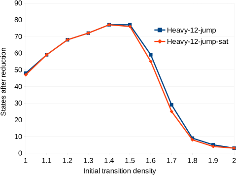
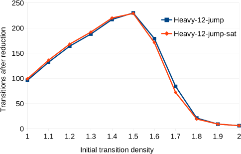
Figure 35. We consider Tabakov-Vardi random Büchi automata with $n=100$, $|\Sigma|=2$, ${\it ad}=0.5$ and ${\it td}=1.0,\dots,2.0$. The x-axis is the transition density of the original automata. In the upper/lower picture the y-axis is the average number of states/transitions of the reduced automata after applying Heavy-12-jump and Heavy-12-jump-sat, respectively. There is hardly any difference between the methods for ${\it td}<1.4$ or ${\it td}>2.0$. Every data point is the average of $1000$ automata.

In contrast, the saturation methods have a significant effect for NFA, as shown in Fig. 36. For transition densities ${\it td}\leq 1.4$ the number of states is marginally reduced at the expense of having a moderately higher number of transitions. For $1.5\leq{\it td}\leq 1.9$ both states and transitions are significantly reduced. For ${\it td}\geq 2.0$ there is no difference, because the automata produced by Heavy-12-jump are already very small. In the interesting region of $1.5\leq{\it td}\leq 1.9$, Heavy-12-jump-sat yields automata with fewer states than Heavy-12-jump in about 30%–60% of the cases, while the number of transitions is only larger in 8%-10% of the cases.

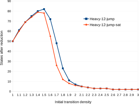
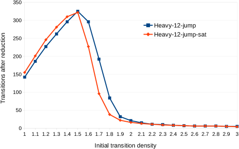
Figure 36. We consider Tabakov-Vardi random NFA with $n=100$, $|\Sigma|=2$, ${\it ad}=0.5$ and ${\it td}=1.0,\dots,3.0$. The x-axis is the transition density of the original automata. In the upper/lower picture the y-axis is the average number of states/transitions of the reduced automata after applying Heavy-12-jump and Heavy-12-jump-sat, respectively. Every data point is the average of $1000$ automata.

In Fig. 37 we compare the speed of Heavy-12-jump and Heavy-12-jump-sat on Büchi automata and NFA, respectively. The results heavily depend on the transition density of the input automata, but in the interesting region of $1.5\leq{\it td}\leq 1.8$, Heavy-12-jump-sat is about 2-4 times slower.

Büchi automata

Finite automata

Figure 37. We consider Tabakov-Vardi random Büchi automata (upper picture) and Tabakov-Vardi random NFA (lower picture) with $n=100$, $|\Sigma|=2$, ${\it ad}=0.5$ and ${\it td}=1.0,\dots,3.0$. The x-axis is the transition density of the original automata while the y-axis is the average time (in ms) to reduce the automata with Heavy-12-jump and Heavy-12-jump-sat, respectively. Every data point is the average of $1000$ automata. Java 7 on Intel 2 Q8300, 2.50GHz.

11. Notes on the Implementation

The tools

Our tools Reduce and RABIT [15] implement the reduction algorithm of Sections 7 and 10 and the inclusion testing algorithm of Sec. 8, respectively. They are distributed in one package, written in Java (version $\geq 7$) and are licensed under the GPLv2.

The Reduce and RABIT tools currently support only the .ba format to describe automata. This format is also supported by GOAL [68]. However, the package contains a utility to convert NFA in .ba format into the .timbuk format used by Libvata [52]. The .ba format is very basic. First it gives the unique initial state. Then comes a list of labeled transitions (one per line) and then the list of accepting states (one per line). Example:

[1]
a,[1]->[2]
b,[2]->[1]
c,[1]->[3]
[2]
[3]

The default reduction algorithm in Reduce is Heavy-k-jump. Other versions like Heavy-k, Heavy-k-jump-sat and a more aggressive version Heavy-k-jump-sat2 can be invoked with options -nojump, -sat and -sat2, respectively. By default it assumes that the input is an NBA. It switches to NFA with the option -finite. The lookahead $k\geq 1$ is given as a parameter. Example: java -jar Reduce.jar example.ba 12 -sat reduces the NBA example.ba with Heavy-12-jump-sat.

The tool RABIT tests inclusion between NBA (or NFA with option -finite). Since it implements many optimizations, it should be invoked with option -fast for best performance. (The default is no optimization, which is very slow.) The lookahead may be specified as a parameter, but by default RABIT uses a heuristic that depends on the sizes and shapes of the input automata. Example: java -jar RABIT.jar A.ba B.ba -fast -jf tests inclusion between the NBA A.ba and B.ba. The additional option -jf has the effect that, after the automata reduction, a new thread is created that runs in parallel to the Ramsey-based antichain method. This thread alternatingly checks the GFI $\preceq^{k\textrm{-}\mathsf{bw}\textrm{-}\mathsf{c}}$-jumping $k$-lookahead fair simulation and the segmented jumping $k$-lookahead fair simulation from Sec. 8.2 for an ever increasing $k=1,2,3,\dots$. (Both threads stop as soon as one of them finds a solution.)

Algorithmic issues

The most critical part of the code is the computation of the $k$-lookahead simulations, since this takes the majority of the time on non-trivial cases. It becomes computationally feasible by using several optimizations described informally below. For details the reader is referred to [15] (algorithms/Simulation.java and algorithms/ParallelSimulation.java).

• We represent binary relations between states by boolean matrices, i.e., $(p,q)$ is in the relation iff the matrix element $(p,q)$ is true. By using the $\mu$-calculus characterization of lookahead simulations in Sec. 6.4, they can be computed by a fixpoint iteration that converges to the lookahead simulation. E.g., for direct simulation one starts with all matrix elements set to true and refines downward. (It is more complex for delayed- and fair simulations.) This takes place in situ, i.e., there is only one copy of the matrix. Thus changing an element in the matrix possibly affects tests and changes of other matrix elements already in the same round of the iteration, instead of the next round. This reduces the number of iterations significantly. (Achieving this in situ effect might be a problem for certain types of symbolic representations, e.g., BDDs.)

• Consider one round of the fixpoint refinement for $k$-lookahead direct simulation. In every such refinement round one needs to check, for every matrix element $(p,q)$ that is still true, whether it should remain true. As explained in Sec. 6.3, for every check of a pair of states $(p,q)$, Spoiler builds his attacks incrementally, i.e., he explores the tree of all possible attacks starting at $p$ by depth-first search up-to depth $k$. For every partial Spoiler attack in this tree, Duplicator searches for a possible defense. Whenever Duplicator can defend (from $q$) against a branch of non-maximal depth, deeper exploration of this branch is omitted. Thus, most of these checks of $(p,q)$ are resolved without exploring the full tree of all attacks from $p$ up-to maximal depth. The following item elaborates different ways how Duplicator can search for a valid defense.

• Given an attack by Spoiler from some state $p$ of some depth $k^{\prime}\leq k$, Duplicator needs to check whether there is a defense from state $q$. A basic algorithm would explore the tree of Duplicator’s moves up-to depth $k^{\prime}$ (and stop once a defense is found). This basic version is implemented in [15], but not normally used (except in cases of very small lookahead), because other versions are often more efficient. The basic version is wasteful (for higher lookahead), because many of Spoiler’s attacks share common prefixes. A more efficient variant (also implemented in [15]) views lookahead simulation as a special case of multipebble simulation, as explained in Remark 6.5. When checking a pair of states $(p,q)$, Duplicator maintains and propagates several pebbles (starting with just one pebble on state $q$) that encode all her possible moves against Spoiler’s current attack from $p$ (up-to depth $k$). Unlike in general multipebble simulation, this use of pebbles is local to the current round of the game, since Duplicator needs to commit to just one pebble after at most $k$ steps.

  This version needs to efficiently handle many sets of pebbles, i.e., subsets of states of the automaton. In an automaton with $n$ states, the states are represented by integers in the set $\{0,\dots,n-1\}$, and sets of pebbles as subsets thereof. The only needed set operations are to add elements and to iterate through all elements of a set, but not to explicitly check membership. Java generic sets are not optimal here, due to their internal overhead (here the elements are just integers and typically $n\leq 30000$). Our implementation uses a combination of integer arrays (to describe a list of size $|S|$; for sets $S$ with $|S|^{2}\leq 4n$) and boolean arrays (of length $n$; otherwise) to represent these sets. In the former case, adding a new element is $\mathcal{O}(|S|)$ (since duplicates must be avoided), but iterating through the set is optimal. Thus it is used only for sets that are small, relative to $n$. In the latter case, adding a new element is $\mathcal{O}(1)$, but iterating through the set takes $\mathcal{O}(n)$ steps (instead of $\mathcal{O}(|S|)$ steps), which is inefficient if $|S|\ll n$. So this representation is used only for larger sets. Since new sets are derived from previous sets by the propagation of the pebbles in the automaton, it is possible to predict (roughly, but reasonably accurately) whether a new set will be small or large in the sense described above.

• Even before the main fixpoint refinement loop starts, one can do a quick pre-processing step that sets many matrix elements to false. If there exists a short word $w$ that can be read from state $p$ but not from state $q$ then it is trivial that $q$ cannot simulate $p$. Our implementation checks this condition for all words up-to a short length, typically 4-8 (depending on the size of the alphabet). The parallel version (see below) does this operation in a separate thread with words $w$ of increasing length (up-to a certain maximum depending on memory requirements).

• Finally, the iterations over the boolean matrix can be parallelized. The matrix is split into many small parts, and each part is handled by a worker-thread from the pool of available worker threads. This uses Java 7 fork-join concurrency and is invoked by the option -par. While each worker-thread writes only to a small part of the matrix, it still needs read access to the whole matrix. Thus the computation cannot easily be distributed, and shared memory access is still a bottleneck. Due to the monotonicity of the fixpoint refinement algorithm, missed updates are not a problem in the parallel version. The parallel version can be several times faster than the single-threaded one, depending on the hardware and on the input instance. However, all our benchmarks were done with the single-threaded version.

An optimized algorithm to compute ordinary simulations (i.e., with lookahead $k=1$) was described in [36, 38]. We explain its main idea for the case of forward direct simulation. When some matrix elements are changed (from true to false) in an iteration of the fixpoint refinement, then only some elements may change in the next round, while other elements cannot possibly change (yet) because they are not directly affected by the recently changed elements. By keeping track of these dependencies, one can avoid redundant tests of elements that will not change (or at least not yet in this iteration). Our implementation uses this technique only in the case of lookahead $k=1$, but not for higher lookaheads, because the dependency information becomes more complex and keeping track of it is not cost-effective. Worse yet, at higher lookaheads the computation time is not evenly distributed over all matrix elements (i.e., pairs of states). Instead the distribution is highly skewed towards a minority of hard cases. Typically, these are pairs of states where lookahead simulation does not hold, but where non-simulation is only established very late, i.e., after many iterations. In many earlier iterations Duplicator still wins easily (in small time) and the element stays true. Avoiding these redundant tests would yield only a small benefit, but still incur the required overhead. The element is only set to false in a late iteration where Duplicator finally admits defeat after having vainly searched through the entire tree of all possible candidates for a defense (against a certain Spoiler attack) up-to the maximal allowed lookahead. This last test is thus a costly operation that cannot be avoided.

12. Conclusion and Future Work

Our automata reduction technique Heavy-k, and its extensions Heavy-k-jump, Heavy-k-jump-sat and Heavy-k-jump-sat2, perform significantly better than previous methods implemented in GOAL [68]. In particular, they can be applied to solve PSPACE-complete automata problems like language inclusion for much larger instances than before. Our tools Reduce and RABIT [15] implement these algorithms in Java (version $\geq 7$) and are licensed under the GPLv2.

Future work includes more efficient algorithms for computing lookahead simulations by using symbolic representations of the relations/automata by BDDs or related formalisms. It would also be very useful to have a practically feasible way to compute under-approximations of language inclusion for NBA/NFA that are orthogonal to multipebble/lookahead-simulations. Then one could obtain an even better approximation by considering the transitive closure of the union of all approximations.

Quotienting techniques for alternating automata over infinite words are well-understood  [31, 32, 18] (cf. also [5, 6]). An interesting research direction is to extend our transition pruning and saturation methods from nondeterministic to alternating finite, Büchi, generalized Büchi, and parity automata.

Finally, transition pruning techniques have more recently been applied to reduce automata on finite trees [8] and infinite trees [7].

Acknowledgments.

We acknowledge the anonymous reviewers for their extensive comments on earlier drafts of this article.

References

- [1] Spot: a platform for LTL and -automata manipulation. https://spot.lrde.epita.fr/.
- [2] P. A. Abdulla, Y.-F. Chen, L. Clemente, L. Holík, C.-D. Hong, R. Mayr, and T. Vojnar. Simulation Subsumption in Ramsey-Based Büchi Automata Universality and Inclusion Testing. In T. Touili, B. Cook, and P. Jackson, editors, Computer Aided Verification, volume 6174 of LNCS, pages 132–147, 2010.
- [3] P. A. Abdulla, Y.-F. Chen, L. Clemente, L. Holík, C.-D. Hong, R. Mayr, and T. Vojnar. Advanced Ramsey-based Büchi Automata Inclusion Testing. In J.-P. Katoen and B. König, editors, International Conference on Concurrency Theory, volume 6901 of LNCS, pages 187–202, Sept. 2011.
- [4] P. A. Abdulla, Y.-F. Chen, L. Holík, R. Mayr, and T. Vojnar. When simulation meets antichains. In TACAS, volume 6015 of LNCS, pages 158–174, 2010.
- [5] P. A. Abdulla, Y.-F. Chen, L. Holík, and T. Vojnar. Mediating for reduction (on minimizing alternating Büchi automata). In FSTTCS, volume 4 of LIPIcs, pages 1–12. Schloss Dagstuhl - Leibniz-Zentrum fuer Informatik, 2009.
- [6] P. A. Abdulla, Y.-F. Chen, L. Holík, and T. Vojnar. Mediating for reduction (on minimizing alternating Büchi automata). Theor. Comput. Sci., 552(0):26–43, 2014.
- [7] R. Almeida. Efficient algorithms for hard problems in nondeterministic tree automata. PhD thesis, School of Informatics. University of Edinburgh, UK, 2017. http://hdl.handle.net/1842/28794.
- [8] R. Almeida, L. Holík, and R. Mayr. Reduction of nondeterministic tree automata. In Proc. of TACAS 2016, volume 9636 of LNCS, 2016. arXiv 1512.08823.
- [9] T. Babiak, M. Křetínský, V. Řehák, and J. Strejček. LTL to Büchi automata translation: Fast and more deterministic. In Proceedings of TACAS 2012, volume 7214 of LNCS, pages 95–109. Springer-Verlag, 2012.
- [10] F. Blahoudek, A. Duret-Lutz, M. Křetínský, and J. Strejček. Is there a best Büchi automaton for explicit model checking? In In Proc. of SPIN’14, SPIN 2014, pages 68–76, New York, NY, USA, 2014. ACM.
- [11] F. Bonchi and D. Pous. Checking NFA equivalence with bisimulations up to congruence. In Principles of Programming Languages (POPL), Rome, Italy. ACM, Jan. 2013.
- [12] N. Bousquet and C. Löding. Equivalence and inclusion problem for strongly unambiguous Büchi automata. In A.-H. Dediu, H. Fernau, and C. Martín-Vide, editors, In Proc. of LATA’10, pages 118–129, Berlin, Heidelberg, 2010. Springer Berlin Heidelberg.
- [13] J. Brzozowski and N. Santean. Predictable semiautomata. Theor. Comput. Sci., 410(35):3236–3249, 2009.
- [14] D. Bustan and O. Grumberg. Simulation-based minimization. ACM Trans. Comput. Logic, 4:181–206, April 2003.
- [15] Y.-F. Chen and R. Mayr. RABIT/Reduce: Tools for language inclusion testing and reduction of nondeterministic Büchi automata and NFA. http://www.languageinclusion.org/doku.php?id=tools.
- [16] L. Clemente. Büchi Automata Can Have Smaller Quotients. In L. Aceto, M. Henzinger, and J. Sgall, editors, ICALP, volume 6756 of LNCS, pages 258–270. Springer-Verlag, 2011.
- [17] L. Clemente. Generalized Simulation Relations with Applications in Automata Theory. PhD thesis, University of Edinburgh, 2012.
- [18] L. Clemente and R. Mayr. Multipebble Simulations for Alternating Automata - (Extended Abstract). In International Conference on Concurrency Theory, volume 6269 of LNCS, pages 297–312. Springer-Verlag, 2010.
- [19] L. Clemente and R. Mayr. Advanced automata minimization. In 40th Annual ACM SIGPLAN-SIGACT Symposium on Principles of Programming Languages, POPL, pages 63–74. ACM, Jan. 2013.
- [20] L. Clemente and R. Mayr. Efficient reduction of nondeterministic automata with application to language inclusion testing. arXiv, 1711.09946, 2018. https://arxiv.org/abs/1711.09946.
- [21] J.-M. Couvreur. On-the-fly verification of linear temporal logic. In Proceedings of the Wold Congress on Formal Methods in the Development of Computing Systems-Volume I - Volume I, FM ’99, pages 253–271, London, UK, UK, 1999. Springer-Verlag.
- [22] D. L. Dill, A. J. Hu, and H. Wont-Toi. Checking for Language Inclusion Using Simulation Preorders. In Computer Aided Verification, volume 575 of LNCS. Springer-Verlag, 1991.
- [23] L. Doyen and J.-F. Raskin. Antichains Algorithms for Finite Automata. In Tools and Algorithms for the Construction and Analysis of Systems, volume 6015 of LNCS, pages 2–22. Springer-Verlag, 2010.
- [24] K. Etessami. A Hierarchy of Polynomial-Time Computable Simulations for Automata. In International Conference on Concurrency Theory, volume 2421 of LNCS, pages 131–144. Springer-Verlag, 2002.
- [25] K. Etessami and G. Holzmann. Optimizing Büchi Automata. In International Conference on Concurrency Theory, volume 1877 of LNCS, pages 153–168. Springer-Verlag, 2000.
- [26] K. Etessami, T. Wilke, and R. A. Schuller. Fair Simulation Relations, Parity Games, and State Space Reduction for Büchi Automata. SIAM J. Comput., 34(5):1159–1175, 2005.
- [27] S. Fogarty, O. Kupferman, M. Y. Vardi, and T. Wilke. Unifying Büchi Complementation Constructions. In M. Bezem, editor, Computer Science Logic, volume 12 of LIPIcs, pages 248–263. Schloss Dagstuhl–Leibniz-Zentrum fuer Informatik, 2011.
- [28] S. Fogarty and M. Vardi. Büchi Complementation and Size-Change Termination. In S. Kowalewski and A. Philippou, editors, Tools and Algorithms for the Construction and Analysis of Systems, volume 5505 of LNCS, pages 16–30. Springer-Verlag, 2009.
- [29] S. Fogarty and M. Y. Vardi. Efficient Büchi Universality Checking. In Tools and Algorithms for the Construction and Analysis of Systems, volume 6015 of LNCS, pages 205–220, 2010.
- [30] W. Fridman, C. Löding, and M. Zimmermann. Degrees of Lookahead in Context-free Infinite Games. In M. Bezem, editor, Proc. of CSL’11, volume 12 of LIPIcs, pages 264–276, Dagstuhl, Germany, 2011. Schloss Dagstuhl–Leibniz-Zentrum fuer Informatik.
- [31] C. Fritz and T. Wilke. Simulation Relations for Alternating Büchi Automata. Theor. Comput. Sci., 338(1-3):275–314, 2005.
- [32] C. Fritz and T. Wilke. Simulation relations for alternating parity automata and parity games. In O. Ibarra and Z. Dang, editors, In Proc. of DLT’06, volume 4036 of LNCS, pages 59–70. Springer Berlin / Heidelberg, 2006.
- [33] P. Gastin and D. Oddoux. Fast LTL to Büchi automata translation. In CAV, volume 2102 of LNCS, pages 53–65. Springer, 2001.
- [34] Ç. E. Gerede, R. Hull, O. H. Ibarra, and J. Su. Automated composition of e-services: Lookaheads. In Proc. of ICSOC ’04, ICSOC ’04, pages 252–262, New York, NY, USA, 2004. ACM.
- [35] S. Gurumurthy, R. Bloem, and F. Somenzi. Fair simulation minimization. In Proc. of CAV’02, volume 2404 of LNCS, pages 610–624. Springer, 2002.
- [36] M. R. Henzinger, T. A. Henzinger, and P. W. Kopke. Computing simulations on finite and infinite graphs. In Foundations of Computer Science, FOCS ’95, Washington, DC, USA, 1995. IEEE Computer Society.
- [37] T. A. Henzinger, O. Kupferman, and S. K. Rajamani. Fair Simulation. Information and Computation, 173:64–81, 2002.
- [38] L. Holík and J. Šimáček. Optimizing an LTS-simulation algorithm. Technical Report FIT-TR-2009-03, Brno University of Technology, 2009. http://www.fit.vutbr.cz/research/view_pub.php.en?id=9085.
- [39] M. Holtmann, L. Kaiser, and W. Thomas. Degrees of lookahead in regular infinite games. LMCS, 8(3:24):1–15, Sept. 2012.
- [40] G. Holzmann. The SPIN Model Checker. Addison-Wesley, 2004.
- [41] J. E. Hopcroft. An algorithm for minimizing states in a finite automaton. Technical report, Stanford, CA, USA, 1971.
- [42] F. A. Hosch and L. H. Landweber. Finite delay solutions for sequential conditions. In Proc. of ICALP’72, pages 45–70, 1972.
- [43] M. Hutagalung, M. Lange, and E. Lozes. Revealing vs. Concealing: More Simulation Games for Büchi Inclusion. In A.-H. Dediu, C. Martín-Vide, and B. Truthe, editors, Proc. of LATA’13, volume 7810 of LNCS, pages 347–358. Springer, 2013.
- [44] M. Hutagalung, M. Lange, and E. Lozes. Buffered simulation games for Büchi Automata. In Ésik, Zoltán and Fülöp, Zoltán, editors, Proc. of AFL’14, volume 151 of EPTCS, pages 286–300. Open Publishing Association, 2014.
- [45] T. Jiang and B. Ravikumar. Minimal NFA Problems are Hard. In J. Albert, B. Monien, and M. Artalejo, editors, ICALP, volume 510 of LNCS, pages 629–640. Springer-Verlag, 1991.
- [46] S. Juvekar and N. Piterman. Minimizing Generalized Büchi Automata. In Computer Aided Verification, volume 4414 of LNCS, pages 45–58. Springer-Verlag, 2006.
- [47] F. Klein and M. Zimmermann. How much lookahead is needed to win infinite games? In M. M. Halldórsson, K. Iwama, N. Kobayashi, and B. Speckmann, editors, Proc. of ICALP’15, volume 9135 of LNCS, pages 452–463. Springer, 2015.
- [48] F. Klein and M. Zimmermann. What are Strategies in Delay Games? Borel Determinacy for Games with Lookahead. In S. Kreutzer, editor, Proc. of CSL’15, volume 41 of LIPIcs, pages 519–533, Dagstuhl, Germany, 2015. Schloss Dagstuhl–Leibniz-Zentrum fuer Informatik.
- [49] O. Kupferman and M. Vardi. Verification of Fair Transition Systems. In Computer Aided Verification, volume 1102 of LNCS, pages 372–382. Springer-Verlag, 1996.
- [50] R. Kurshan. Complementing deterministic Büchi automata in polynomial time. Journal of Computer and System Sciences, 35(1):59–71, 1987.
- [51] C. S. Lee, N. D. Jones, and A. M. Ben-Amram. The size-change principle for program termination. In Proc. of POPL’01, pages 81–92. ACM, 2001.
- [52] O. Lengál, J. Šimáček, and T. Vojnar. Libvata: highly optimised non-deterministic finite tree automata library. http://www.fit.vutbr.cz/research/groups/verifit/tools/libvata/, 2015.
- [53] J. Leroux and G. Point. TaPAS: The Talence Presburger Arithmetic Suite. In Proceedings of the 15th International Conference on Tools and Algorithms for the Construction and Analysis of Systems (TACAS), volume 5505 of LNCS. Springer, 2009.
- [54] C. Löding. Efficient minimization of deterministic weak omega-automata. Inf. Process. Lett., 79(3):105–109, July 2001.
- [55] C. Löding and S. Repke. Decidability Results on the Existence of Lookahead Delegators for NFA. In A. Seth and N. K. Vishnoi, editors, FSTTCS’13, volume 24 of LIPIcs, pages 327–338, Dagstuhl, Germany, 2013. Schloss Dagstuhl–Leibniz-Zentrum fuer Informatik.
- [56] A. R. Meyer and L. J. Stockmeyer. The equivalence problem for regular expressions with squaring requires exponential space. In Proceedings of the 13th Annual Symposium on Switching and Automata Theory, SWAT ’72, pages 125–129, Washington, DC, USA, 1972. IEEE Computer Society.
- [57] R. Milner. Communication and Concurrency. Prentice Hall, 1989.
- [58] I. Niven. Mathematics of Choice. The Mathematical Association of America, 1965.
- [59] D. Park. Concurrency and automata on infinite sequences. In Proceedings of the 5th GI-Conference on Theoretical Computer Science, pages 167–183, London, UK, UK, 1981. Springer-Verlag.
- [60] N. Piterman. From nondeterministic Büchi and Streett automata to deterministic parity automata. In LICS, pages 255–264. IEEE, 2006.
- [61] J. Rathke, P. Sobociński, and O. Stephens. Compositional reachability in Petri Nets. In J. Ouaknine, I. Potapov, and J. Worrell, editors, Proc. of RP’14, volume 8762 of LNCS, pages 230–243. Springer, 2014.
- [62] B. Ravikumar and N. Santean. Deterministic simulation of a NFA with k–symbol lookahead. In J. van Leeuwen, G. Italiano, W. van der Hoek, C. Meinel, H. Sack, and F. Plášil, editors, Proc. of SOFSEM’07, volume 4362 of LNCS, pages 488–497. Springer, 2007.
- [63] R. Sebastiani and S. Tonetta. More deterministic vs. smaller Büchi automata for efficient LTL model checking. In Correct Hardware Design and Verification Methods, volume 2860 of LNCS, 2003.
- [64] A. P. Sistla, M. Y. Vardi, and P. Wolper. The complementation problem for Büchi automata with applications to temporal logic. Theor. Comput. Sci., 49:217–237, Jan. 1987.
- [65] F. Somenzi and R. Bloem. Efficient Büchi Automata from LTL Formulae. In Computer Aided Verification, volume 1855 of LNCS, pages 248–263. Springer-Verlag, 2000.
- [66] D. Tabakov and M. Vardi. Model Checking Büchi Specifications. In LATA, volume Report 35/07. Research Group on Mathematical Linguistics, Universitat Rovira i Virgili, Tarragona, 2007.
- [67] W. Thomas. Automata on Infinite Objects, Handbook of theoretical computer science (vol. B), Chapter 4. MIT Press Cambridge, MA, USA, 1990.
- [68] Y.-K. Tsay, Y.-F. Chen, M.-H. Tsai, W.-C. Chan, and C.-J. Luo. GOAL extended: Towards a research tool for omega automata and temporal logic. In C. Ramakrishnan and J. Rehof, editors, Tools and Algorithms for the Construction and Analysis of Systems, volume 4963 of LNCS, pages 346–350. Springer-Verlag, 2008.
- [69] Y.-K. Tsay, M.-H. Tsai, J.-S. Chang, and Y.-W. Chang. Büchi store: An open repository of Büchi automata. In P. A. Abdulla and K. Leino, editors, Tools and Algorithms for the Construction and Analysis of Systems, volume 6605 of LNCS, pages 262–266. Springer-Verlag, 2011. 10.1007/978-3-642-19835-9_23 http://buchi.im.ntu.edu.tw/.
- [70] Y.-K. Tsay, M.-H. Tsai, J.-S. Chang, Y.-W. Chang, and C.-S. Liu. Büchi Store: An open repository of -automata. International Journal on Software Tools for Technology Transfer, 15(2):109–123, 2013. http://buchi.im.ntu.edu.tw/.
- [71] M. D. Wulf, L. Doyen, T. A. Henzinger, and J.-F. Raskin. Antichains: A new algorithm for checking universality of finite automata. In Proc. of CAV 2006, volume 4144 of LNCS, pages 17–30. Springer-Verlag, 2006.