Integrable time-dependent quantum Hamiltonians

Abstract

We formulate a set of conditions under which dynamics of a time-dependent quantum Hamiltonian are integrable. The main requirement is the existence of a nonabelian gauge field with zero curvature in the space of system parameters. Known solvable multistate Landau-Zener models satisfy these conditions. Our method provides a strategy to incorporate time-dependence into various quantum integrable models, so that the resulting non-stationary Schrödinger equation is exactly solvable. We also validate some prior conjectures, including the solution of the driven generalized Tavis-Cummings model.

Quantum coherent dynamics controlled by strong time-dependent fields can be realized and explored nowadays in systems of considerable complexity kinoshita2006 ; monaco ; ligner ; weiler ; widera ; Gring:2012 ; Trotzky:2012 ; shimano2013 . Time-dependent parameters play a critical role in NMR NMR-LZ , quantum information processing dot-lz-exp1 ; nichol ; zhou ; gaudreau ; LZ-metrology ; forster ; riberio ; wubs ; Wernsdorfer ; annealing-LZ ; q-phaset , molecular dynamics book-LZ ; child ; nikitin and cold atom experiments regal ; zwierlein ; atomic . On the theory side, quantum dynamics of time-dependent many-body Hamiltonians, especially their exact analytical description, present considerable challenges. In contrast, exact solutions of significant relevance to experiment inform our understanding of stationary states, e.g., Bethe’s Ansatz solution of paradigmatic models gaudin ; bethe2 ; sutherland . Nontrivial exact results have been also obtained for quantum quenches, such as the Generalized Gibbs Ensemble description of the dynamics of the spin-1/2 Heisenberg chain ilievski2 and quantum quench phase diagrams of BCS superconductors quench1 . Such methods, unfortunately, do not apply to a Hamiltonian with continuous time-dependence.

In this letter, we propose an approach for solving the non-stationary Shrödinger equation exactly for a certain class of time-dependent Hamiltonians. This approach allows us to make parameters of a quantum integrable model, e.g., the BCS and generalized Tavis-Cummings Hamiltonians, vary in time in such a way that resulting dynamics are exactly solvable. Here we focus primarily on the scattering problem, i.e. on determining the time-evolution over a specific time interval.

Important examples of driven systems are matrix Hamiltonians linear in time, $H(t)=A+Bt$, where $A$ and $B$ are time-independent Hermitian $N\times N$ matrices. The problem of finding the scattering matrix that relates the state of the system at $t=+\infty$ to that at $t=-\infty$ is called then the multistate Landau-Zener problem. The $2\times 2$ problem was solved by Landau, Zener, Majorana and Stückelberg in 1932 landau ; zener ; Majorana ; stuckelberg . For $N\geq 3$ the solution is known only for special choices of $A$ and $B$. Earliest examples include Demkov-Osherov do ; be , bow-tie bow-tie , generalized bow-tie gbow-tie1 ; gbow-tie , composite multiparticle , and infinite chain lz-chain models. In a more recent work yuzbashyan-LZ , it was shown that nontrivial solvable models belong to families of mutually commuting Hamiltonians linear or quadratic in $t$. It was therefore conjectured that quantum integrability understood as the existence of nontrivial time-dependent commuting partners shastry ; haile1 ; haile ; shastry1 is a necessary condition for the multistate Landau-Zener solvability. In a parallel development, methods to solve and search for new models were discovered six-LZ ; quest-LZ ; constraints and since then the number of such models has grown rapidly four-LZ ; DTCM ; DTCM1 ; chen-largeLZ .

Our approach provides a unified framework to derive exact solutions for all these models and supports the conjecture made in yuzbashyan-LZ . Below, we first formulate our approach and then discuss various many-body and matrix models that fit into it. To illustrate our technique, we solve the scattering problem for two nontrivial models – the generalized Tavis-Cummings Hamiltonian with a linear drive and a new 4-state Hamiltonian linear in $t$. We conclude with several general observations and an outline of the idea of the solution for arbitrary $t$.

Consider a Hamiltonian $\hat{H}(t,\vec{x})$ that, in addition to time, depends on $M$ real parameters $(x^{1},\dots,x^{M})=\vec{x}$. For example, in the multistate Landau-Zener problem these can be certain matrix elements of $A$ and $B$. The main idea is to embed the non-stationary Shrödinger equation for $\hat{H}(t,\vec{x})$ into a set of multi-time Shrödinger equations

$$i\partial_{j}\Psi(\bm{x})=\hat{H}_{j}\Psi(\bm{x}),\;\phantom{\sum}j=0,1,\ldots,M,$$ (1)

where $\bm{x}=(t,\vec{x})$, $\partial_{j}\equiv\partial/\partial x^{j}$, $x^{0}=t$, $\hat{H}_{0}\equiv\hat{H}(t,\vec{x})$, and Hamiltonians $\hat{H}_{j}$ are independent. In other words, the first equation ($j=0$) is the non-stationary Shrödinger equation, while the rest are auxiliary Shrödinger equations that help us solve it exactly. Taking the derivative of Eq. (1) with respect to $x^{k}$, we derive consistency conditions

$$\partial_{j}\hat{H}_{k}-\partial_{k}H_{j}-i[\hat{H}_{k},\hat{H}_{j}]=0,\quad k,j=0,\ldots,M.$$ (2)

These conditions are sufficient and necessary for system (1) to possess a joint solution for any initial condition petrat ; deform-book . We may view them as a generalization of the notion of integrals of motion for time-dependent quantum Hamiltonians.

A formal solution of Eq. (1) along a path in the space of real parameters $\bm{x}$ that starts at a reference point $\bm{x_{0}}$ is an ordered exponential

$$\Psi(\bm{x})=T\exp\left(-i\int_{{\cal P}}\hat{H}_{j}dx^{j}\right)\Psi(\bm{x_{0}}),$$ (3)

where we assume summation over repeated indices. Treating Hamiltonians $\hat{H}_{j}$ as matrix components of a nonabelian gauge field ${\cal A}(\bm{x})$, ${\cal A}_{j}=-i\hat{H}_{j}$, we interpret Eq. (2) as the zero curvature condition ${\cal F}_{jk}\equiv\partial_{j}{\cal A}_{k}-\partial_{k}{\cal A}_{j}-[{\cal A}_{j},{\cal A}_{k}]=0$, so that $\Psi(\bm{x})$ in Eq. (3) is independent of the integration path ${\cal P}$ as long as its endpoints are fixed. Similar zero curvature integrability condition is also well known in soliton physics faddeev-book . It is precisely this freedom to choose a suitable path that enables us to explicitly solve the scattering problem.

Further, consider a path ${\cal P}_{\tau}$ parameterized by a variable $\tau$

$${\cal P}_{\tau}:\quad x^{j}(\tau)=v^{j}\tau+x_{0}^{j},\quad j=0,\ldots,M,$$ (4)

where $v^{j}$ and $x_{0}^{j}$ are constants. The state vector $\Psi(\tau)=\Psi(\bm{x}(\tau))$ along this path satisfies

$$i\frac{d\Psi(\tau)}{d\tau} = \hat{h}(\tau)\Psi(\tau),$$ (5)

$$\hat{h}(\tau) = \sum_{j}v^{j}\hat{H}_{j}(\bm{x}(\tau)).$$ (6)

Solutions of Eq. (5) follow from those of Eq. (1). Therefore, $\hat{h}(\tau)$ – an arbitrary linear combination of $\hat{H}_{j}$ – is also a solvable time-dependent model just like a linear combination of integrals of motion of a time-independent model is also an integral. Note however that the coefficients $v^{j}$ of this linear combination dictate the time-dependence of $\hat{h}(\tau)$.

An important observation is that complex looking Eq. (1) simplifies considerably when the matrix elements of the Hamiltonians are real. Then, the real and imaginary parts of Eq. (2) yield two separate conditions

$$\left[\hat{H}_{j},\hat{H}_{k}\right] = 0,$$ (7)

$$\partial_{j}\hat{H}_{k}-\partial_{k}\hat{H}_{j}=0, \,\,j,k=0,1,\ldots,M.$$ (8)

These equations suggest a strategy for identifying solvable time-dependent models. First, we note that Eq. (7) is to be supplemented with a notion of a nontrivial commuting partner that weeds out trivial partners (e.g., projectors onto the eigenstates of $\hat{H}$). One way is to restrict the parameter (time) dependence of $\hat{H}_{j}$ to be linear or, more generally, polynomial in $t$. This leads to a systematic classification and explicit construction of commuting families of parameter-dependent matrix Hamiltonians haile ; haile1 ; shastry ; yuzbashyan-LZ , which are interesting candidates for our approach. More generally, any quantum integrable model that contains two or more real parameters is a potential candidate. Such models have an extensive number of integrals of motion that satisfy Eq. (7). If no initial subset of integrals satisfies Eq. (8), we attempt to redefine them by taking various combinations and similarly redefine the parameters to make Eq. (8) work for at least $M=1$. Note that once we declare one of the variables $x^{j}$ to be the physical time, commuting partners $\hat{H}_{j}$ cease to be integrals of motion.

For example, take the generalized Tavis-Cummings model

$$\hat{H}_{\mathrm{TC}}=\sum_{j=1}^{N_{s}}\varepsilon_{j}\hat{s}_{j}^{z}-\omega\hat{a}^{\dagger}\hat{a}+g\!\sum_{j=1}^{N_{s}}(\hat{a}^{\dagger}\hat{s}^{-}_{j}+\hat{a}\hat{s}^{\dagger}_{j}),$$ (9)

where $\hat{a}$ is the boson annihilation operator and $\hat{s}_{j}^{z}$, $\hat{s}_{j}^{\pm}$ are spin-1/2 operators. Its commuting partners are dicke

$$\hat{H}_{j}\!=\!(\varepsilon_{j}\!+\!\omega)\hat{s}_{j}^{z}\!+\!g(\hat{a}^{\dagger}\hat{s}_{j}^{-}\!\!+\!\hat{a}\hat{s}_{j}^{\dagger})\!+\!2g^{2}\!\sum_{k\neq j}\frac{\hat{\bf s}_{j}\cdot\hat{\bf s}_{k}}{\varepsilon_{j}-\varepsilon_{k}}.$$ (10)

Equations (7,8) hold with $M=N_{s}$, $\hat{H}_{0}=\hat{H}_{\mathrm{TC}}$, $\bm{x}=(\omega,\varepsilon_{1},\dots,\varepsilon_{N_{s}})$. Another example is the BCS Hamiltonian. In terms of Anderson pseudospin-1/2 operators it reads

$$\hat{H}_{\mathrm{BCS}}=\sum_{j=1}^{N_{s}}2\varepsilon_{j}\hat{s}_{j}^{z}-\frac{1}{2B}\sum_{j,k}\hat{s}_{j}^{+}\hat{s}_{k}^{-},$$ (11)

where $(2B)^{-1}$ stands for the BCS coupling constant. Its commuting partners are Gaudin magnets gaudin ; integ

$$\hat{H}_{j}=2B\hat{s}_{j}^{z}-\sum_{k\neq j}\frac{\hat{\bf s}_{j}\cdot\hat{\bf s}_{k}}{\varepsilon_{j}-\varepsilon_{k}}.$$ (12)

Now $\hat{H}_{0}=\hat{H}_{\mathrm{BCS}}$ and $x^{0}=B$. Thus, the generalized Tavis-Cummings model with a linear sweep of the bosonic frequency, $\omega=t$, and the BCS Hamiltonian with coupling $\propto 1/t$ both fit into our construction. Similarly, using the commuting partners derived in yuzbashyan-LZ , we verified that the Demkov-Osherov, bow-tie, and generalized bow-tie, as well as Landau-Zener-Coulomb models sinitsyn-14pra ; LZC ; LZC1 ; LZC2 fit into our construction.

A key point of this letter is that zero curvature condition (1) leads to an explicit exact solution of the scattering problem. Consider, e.g., the multistate Landau-Zener model $\hat{H}(t,\vec{x})=\hat{A}(\vec{x})+t\hat{B}(\vec{x})$ for which we need to determine the matrix of transition probabilities $P$ with elements ${P}_{nn^{\prime}}\equiv{P}_{n^{\prime}\rightarrow n}\equiv|S_{nn^{\prime}}|^{2}$. Here $S$ is the scattering matrix between eigenstates at $t=-\infty$ and $t=+\infty$ at some fixed values of the parameters, $\vec{x}=\vec{c}$ be . As discussed above, we are free to choose any path in the space $\bm{x}=(t,\vec{x})$ that connects the points $(-\infty,\vec{c})$ and $(+\infty,\vec{c})$. It is convenient to choose a path ${\cal P}_{\infty}$, such that $|\bm{x}|$ is always large and the time-evolution is adiabatic everywhere, except the neighborhood of isolated points, where scattering takes place. The corresponding scattering problem is typically simple thanks to large $|\bm{x}|$, e.g., it reduces to a $2\times 2$ Landau-Zener problem in the two nontrivial examples we consider below. In general, Eqs. (7,8) enable one to construct a multidimensional version of WKB with simple scattering matrices connecting adiabatic (WKB) solutions in different adiabatic regions suppl .

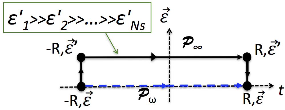
Figure 1: (color online) Paths in the space of parameters $\varepsilon_{j}$ and time used to evaluate transition probabilities for the driven generalized Tavis-Cummings model (9), $\omega=t$. On ${\cal P}_{\omega}$, $\omega$ changes from $-R$ to $+R$, all $\varepsilon_{j}$ are fixed. Since this model is a part of a commuting family of $\hat{H}_{j}$ that satisfies the zero curvature condition, we can deform ${\cal P}_{\omega}$ into a new path ${\cal P}_{\infty}$ without modifying the scattering matrix.

Our first example is the Tavis-Cummings model (9) with linear drive, $\omega=t$. Let $\varepsilon_{1}>\varepsilon_{2}>\dots>\varepsilon_{N_{s}}$. We are interested in the evolution along the path ${\cal P}_{\omega}$ shown in Fig. 1. On this path $\varepsilon_{j}=\mbox{const}$, while $\omega$ changes from $-R$ to $R$. At the end we take the limit $R\to\infty$. This scattering problem was solved in DTCM under the assumption that $\varepsilon_{j}$ are well separated, i.e. $\varepsilon_{1}\gg\varepsilon_{2}\gg\dots\gg\varepsilon_{N_{s}}$. It was further conjectured in DTCM that this is the general solution. We are now in the position to prove this conjecture. To do so, consider the path ${\cal P}_{\infty}$ in Fig. 1 that has the same endpoints as ${\cal P}_{\omega}$. On the first vertical leg of ${\cal P}_{\infty}$, $\varepsilon_{j}$ evolve, keeping the ordering of $\varepsilon_{j}$, until the condition $\varepsilon_{1}\gg\varepsilon_{2}\gg\dots\gg\varepsilon_{N_{s}}$ is met. On the second vertical leg, they evolve back to their initial values. Since $|\omega|$ is large and $\varepsilon_{j}$ are distinct, this evolution is purely adiabatic and does not affect the transition probabilities. On the horizontal leg of ${\cal P}_{\infty}$ the problem is precisely the one solved in DTCM . This proves the above conjecture.

In our second example, we take a previously solved $4\times 4$ multistate Landau-Zener problem four-LZ ; constraints and derive from it a new, more general Hamiltonian by the prescription outlined below Eq. (6). We then proceed to determine the transition probabilities for this new model. Let

$${H}(t,e)=\left(\begin{array}[]{cccc}b_{1}t+e&0&g&-\gamma\\ 0&-b_{1}t+e&\gamma&g\\ g&\gamma&b_{2}t&0\\ -\gamma&g&0&-b_{2}t\end{array}\right),$$ (17)

where $b_{1}$, $b_{2}$, $e$, $g$ and $\gamma$ are constants. To determine if this Hamiltonian fits into our approach, we first search for a nontrivial commuting partner $H_{1}$ linear in $t$. This reduces to a set of linear algebraic equations for parameters of ${H}_{1}$ haile . We find three linearly independent commuting operators. Two of them are trivial – the unit matrix and ${H}$ itself. Therefore, there is a single nontrivial commuting partner, which we determine explicitly. When both $H_{0}\equiv{H}$ and ${H}_{1}$ are linear in $t$ , Eq. (7) implies that their time-dependent parts are diagonal in the same basis. So, to satisfy (8), the parameter $x^{1}$ must be constructed from diagonal time-independent elements of ${H}$. A natural candidate is $x^{1}=e$. Searching then for ${H}_{1}$ that satisfies (8) in the form of a linear combination of the three commuting operators, we find

$${H}_{1}(t,e)\!=\!\left(\!\!\begin{array}[]{cccc}t\!+\!\frac{b_{1}e}{b_{1}^{2}-b_{2}^{2}}&0&\frac{g}{b_{1}-b_{2}}&\frac{-\gamma}{b_{1}+b_{2}}\\ 0&t\!-\!\frac{b_{1}e}{b_{1}^{2}-b_{2}^{2}}&\frac{-\gamma}{b_{1}+b_{2}}&\frac{-g}{b_{1}-b_{2}}\\ \frac{g}{b_{1}-b_{2}}&\frac{-\gamma}{b_{1}+b_{2}}&-\frac{b_{2}e}{b_{1}^{2}-b_{2}^{2}}&0\\ \frac{-\gamma}{b_{1}+b_{2}}&\frac{-g}{b_{1}-b_{2}}&0&\frac{b_{2}e}{b_{1}^{2}-b_{2}^{2}}\end{array}\!\!\right)\!\!.$$ (22)

Let the evolution path be

$${\cal P}_{\tau}:\,\,t=\tau,\,\,e=v\tau+e_{0},$$ (23)

with constant $v$ and $e_{0}$. The Hamiltonian (5) for ${\cal P}_{\tau}$ is

$$h(\tau)\!=\!\!\left(\!\!\begin{array}[]{cccc}\beta_{1}\tau+e_{1}&0&g(1+x)&-\gamma(1+y)\\ 0&\beta_{2}\tau+e_{2}&\gamma(1-y)&g(1-x)\\ g(1+x)&\gamma(1-y)&\beta_{3}\tau+e_{3}&0\\ -\gamma(1+y)&g(1-x)&0&\beta_{4}\tau+e_{4}\end{array}\!\!\right)\!\!,$$ (28)

$$x=\frac{v}{b_{1}-b_{2}},\,\,y=\frac{v}{b_{1}+b_{2}},\,\,\beta_{1,2}=2v\pm b_{1}(1+xy),\,\beta_{3,4}=$$

$$\pm b_{2}(1-xy),\,e_{1,2}=e_{0}(1\pm b_{1}xy/v),\,e_{3,4}=\mp e_{0}b_{2}xy/v.$$

This is a new, previously unsolved model more general than (17), e.g., all couplings (off-diagonal matrix elements) in (28) are distinct. We proceed to solve it with our method.

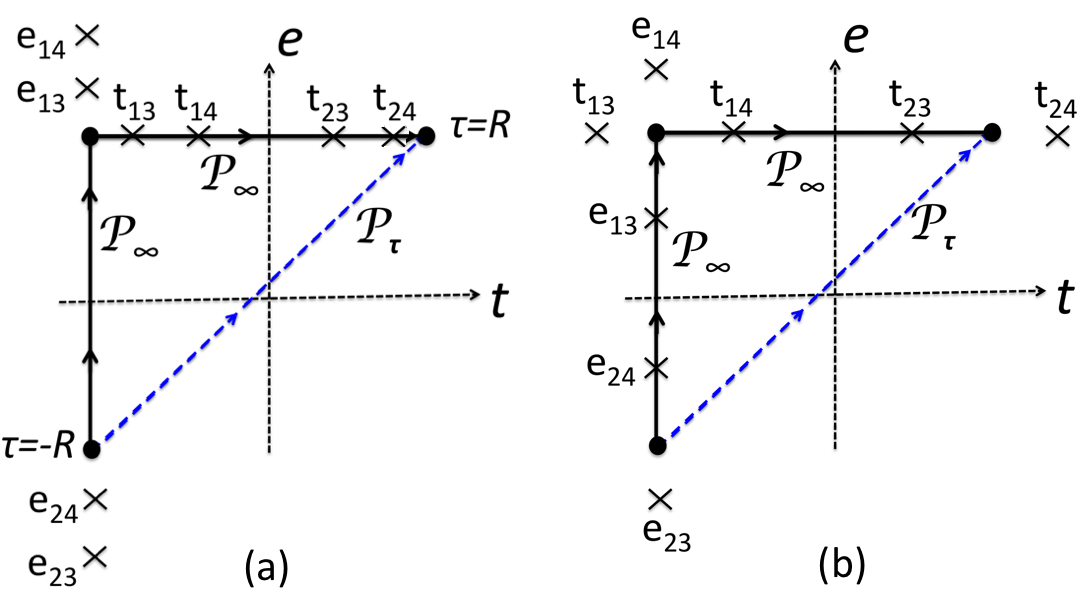
Figure 2: (color online) Paths in the space $(t,e)$ for evaluating transition probabilities for the model (28). On ${\cal P}_{\tau}$, $\tau$ changes from $-R$ to $+R$; all other parameters are fixed. We deform ${\cal P}_{\tau}$ into ${\cal P}_{\infty}$ without affecting the scattering matrix. Points $e_{ij}$ and $t_{ij}$ marked with crosses indicate nonadiabatic Landau-Zener transitions between levels $i$ and $j$ for (a) $v<b_{1}-b_{2}$ and (b) $b_{1}+b_{2}>v>b_{1}-b_{2}$.

Let $b_{1}>b_{2}>0$ and $v>0$. We are interested in the evolution matrix for $h(\tau)$ along the path ${\cal P}_{\tau}$ from $\tau=-R$ to $\tau=R$, see Fig. 2(a), in the limit $R\rightarrow\infty$. Because ${H}_{0}(t,e)$ and ${H}_{1}(t,e)$ satisfy the zero curvature condition, the evolution matrix is the same as that for the path ${\cal P}_{\infty}$. The latter has two pieces. In the vertical one, we set $t=-R$ and vary $e$ from $-vR+e_{0}$ to $vR+e_{0}$. In the horizontal piece, we fix $e=vR+e_{0}$ and vary $t$ from $-R$ to $R$. According to Eq. (3), only ${H}_{1}$ contributes on the first piece and only ${H}_{0}$ on the second. Along ${\cal P}_{\infty}$, diagonal matrix elements of $H_{0}$ and $H_{1}$ (diabatic levels) are large compared to the couplings. Therefore, the levels are well separated, except on disjoined small segments of ${\cal P}_{\infty}$ near points where a pair of the diagonal elements is degenerate. These segments connect adiabatic parts of ${\cal P}_{\infty}$ where the adiabatic approximation is exact in the limit $R\to\infty$. Let us write the state of the system as $\Psi(t,e)=\sum_{k}a_{k}|k\rangle$, where $|k\rangle$ are the eigenstates of the diagonal parts of $H_{0}$ and $H_{1}$ (diabatic eigenstates). Diabatic and adiabatic (instantaneous) eigenstates coincide in adiabatic parts of ${\cal P}_{\infty}$ when $R\to\infty$. In the adiabatic approximation, absolute values of $a_{k}$ remain the same, while their phases evolve with $t$ and $e$.

In the vicinity of degeneracy points, two levels come close and transitions between them become locally possible. The other two levels, however, remain far remote and do not affect these nonadiabatic transitions. Suppose $v<b_{1}-b_{2}$. For this case, we mark the points of diabatic level crossings with crosses in Fig. 2(a). Along ${{\cal P}}_{\infty}$, adiabatic approximation brakes near four points that all have $e=vR+e_{0}$ and

$$t_{13/24}=\mp\frac{vR+e_{0}}{b_{1}-b_{2}},\quad t_{14/23}=\mp\frac{vR+e_{0}}{b_{1}+b_{2}}.$$

The distances between these points are $\propto R$, which means that regions of pairwise nonadiabatic transitions along ${{\cal P}}_{\infty}$ are well apart. Consider, e.g., the evolution of the amplitudes $a_{1}$ and $a_{3}$ near $t_{13}$ that is governed by $H_{0}$. Writing $t=t^{\prime}+t_{13}$ and disregarding the other two levels, we find

$$i\frac{da_{1}}{dt^{\prime}}=b_{1}t^{\prime}a_{1}+ga_{3},\quad i\frac{da_{3}}{dt^{\prime}}=b_{2}t^{\prime}a_{3}+ga_{1},$$ (29)

which is a $2\times 2$ Landau-Zener problem, whose scattering matrix is known explicitly landau ; zener ; Majorana ; stuckelberg . Since the other two levels do not experience nonadiabatic transitions here, they produce only diagonal unit entries in the scattering matrix for evolution through $t_{13}$. The total evolution matrix $S$ for the path ${\cal P}_{\infty}$ factorizes into an ordered product of such pairwise scattering matrices ${S}^{ab}$, where $a,b$ label states experiencing nonadiabatic transitions and diagonal matrices $U^{\alpha,\beta}$ describe adiabatic evolution between points $\alpha$ and $\beta$ on this path, i.e.

$${S}={U}^{R,t_{24}}{S}^{24}{U}^{t_{24},t_{23}}{S}^{23}{U}^{t_{23},t_{14}}{S}^{14}{U}^{t_{14},t_{13}}{S}^{13}{U}^{t_{13},-R}.$$

Trivial phases resulting from the adiabatic evolution drop out from the matrix of transition probabilities and we obtain suppl

$${P}^{v<b_{1}-b_{2}}=\left(\begin{array}[]{cccc}p_{1}p_{2}&0&p_{2}q_{1}&q_{2}\\ 0&p_{1}p_{2}&q_{2}&p_{2}q_{1}\\ p_{2}q_{1}&q_{2}&p_{1}p_{2}&0\\ q_{2}&p_{2}q_{1}&0&p_{1}p_{2}\end{array}\right),$$ (34)

$$p_{1} = e^{-2\pi g^{2}/(b_{1}-b_{2})},\,\,\,p_{2}=e^{-2\pi\gamma^{2}/(b_{1}+b_{2})},\,\,\,q_{1,2}=1-p_{1,2}.$$

This result does not depend on $v$, so it coincides with the solution for the model (17) found in four-LZ ; constraints .

The situation changes for $b_{2}+b_{2}>v>b_{1}-b_{2}$. Now the points of adiabaticity violation $e_{24}$ and $e_{13}$ lie on the first leg of the path ${\cal P}_{\infty}$ as shown in Fig. 2(b). Pairwise transitions near these points are now governed by the Hamiltonian ${H}_{1}$ and the transition probability matrix in this case is different

$${P}^{v>b_{1}-b_{2}}_{v<b_{1}+b_{2}}=\left(\begin{array}[]{cccc}p_{1}p_{2}&q_{1}q_{2}&p_{2}q_{1}&p_{1}q_{2}\\ q_{1}q_{2}&p_{1}p_{2}&p_{1}q_{2}&p_{2}q_{1}\\ p_{2}q_{1}&p_{1}q_{2}&p_{1}p_{2}&q_{1}q_{2}\\ p_{1}q_{2}&p_{2}q_{1}&q_{1}q_{2}&p_{1}p_{2}\end{array}\right).$$ (39)

For $v>b_{1}+b_{2}$, all four points with Landau-Zener transitions lie on the first leg of ${\cal P}_{\infty}$ and

$${P}^{v>b_{1}+b_{2}}=\left(\begin{array}[]{cccc}p_{1}p_{2}&0&q_{1}&p_{1}q_{2}\\ 0&p_{1}p_{2}&p_{1}q_{2}&q_{1}\\ q_{1}&p_{1}q_{2}&p_{1}p_{2}&0\\ p_{1}q_{2}&q_{1}&0&p_{1}p_{2}\end{array}\right).$$ (44)

We see that our approach not only reproduces the previously known solution for the Hamiltonian (17), but also solves a more complex model (28).

Thus, we have identified a symmetry – multi-time evolution with commuting Hamiltonians – that leads to the integrability of unitary dynamics with time-dependent Hamiltonians. Our approach generates numerous new solvable multistate Landau-Zener models. As examples, we solved a four-state model (28) and proved the previously conjectured solution of a combinatorially complex driven Tavis-Cummings model (9), which has important applications in physics of molecular condensates gurarie-LZ ; altland3 . We believe, this symmetry is behind most if not all nontrivial exactly solvable multistate Landau-Zener and Landau-Zener-Coulomb models sinitsyn-14pra ; LZC ; LZC1 ; LZC2 . It explains why in such problems the scattering matrix factorizes into a product of two-state scattering matrices six-LZ – since Eq. (1) allows a choice of an integration path that bypasses the region of complex nonadiabatic dynamics. It also explains why basic known solvable models have commuting partners with simple linear or quadratic dependence on $t$ yuzbashyan-LZ . Indeed, pairs of such operators that also satisfy Eq. (8) lead to relatively simple versions of the WKB approximation necessary to determine scattering matrices. Further, Eq. (6) shows how certain distortions of the parameters quest-LZ give rise to entire families of solvable models.

Finally, we note that when $\hat{H}_{j}$ are isotropic Gaudin magnets [Eq. (12) at $B=0$], the $j=1,\dots,M$ subsystem of Eq. (1) is the famous Knizhnik-Zamolodchikov equation KZ . Its solutions have been obtained using off-shell Bethe’s Ansatz babujian2 . This was generalized to $B\neq 0$ in sedrakyan (see also sierra ) and exploited in gritsev to obtain the dynamics of an isotropic Gaudin magnet with time-dependent $\varepsilon_{i}$. We believe, solutions to Eq. (1), i.e. exact inexplicit solutions of the non-stationary Shrödinger equation at arbitrary $t$, for all time-dependent Hamiltonians discussed in this letter can be obtained by further extending this technique.

Supplemental material for “Integrable time-dependent Hamiltonians”

.1 Multidimensional WKB approximation

In the examples in the main text, we were able to obtain explicit transition probability matrices, because the energy levels of Hamiltonians $\hat{H}_{j}(\bm{x})$ were for the most part well separated at large $|{\bm{x}}|$, making the adiabatic approximation exact when $|{\bm{x}}|\to\infty$. In this section, we study this method generally, starting from the zero curvature condition for real symmetric Hamiltonians, i.e. from Eqs. (7,8) in the main text. We interpret it as a multidimensional WKB method in the real space $\mathbb{R}^{M+1}$. The elements of this space are $\bm{x}=(t,x^{1},\dots,x^{M})$, where $x^{1},\dots,x^{M}$ are the system parameters and $t$ is the time variable. In the ordinary WKB method, the eigenstates of a 1D or a multidimensional completely separable Hamiltonian are proportional to $e^{i{\cal S}(\bm{q},t)}$, where $\bm{q}$ are the generalized coordinates and ${\cal S}(\bm{q},t)$ is the classical action. In our case, we cast the $\bm{x}$-dependence of the components of the wavefunction in the adiabatic basis into the form $e^{i{\cal S}^{a}(\bm{x})}$, where $a=1,\ldots,N$ is the index of the adiabatic level. The quantities ${\cal S}^{a}(\bm{x})$ are single-valued functions thanks to the path-independence of the time-ordered exponential

$$\Psi(\bm{x})=T\exp\left(-i\int_{{\cal P}}\hat{H}_{j}dx^{j}\right)\Psi(\bm{x_{0}}),$$ (45)

[see Eq. (3) in the main text] and they also turn out to be real. We therefore interpret ${\cal S}^{a}(\bm{x})$ as the classical action corresponding to the $a$-th adiabatic level.

Eqs. (7,8) from the main text read

$$[\hat{H}_{j}(\bm{x}),\hat{H}_{k}(\bm{x})]=0, \quad j,k=0,1,\ldots,M.$$ (46)

$$\partial_{j}\hat{H}_{k}(\bm{x})-\partial_{k}\hat{H}_{j}(\bm{x})=0.$$ (47)

Eq. (46) implies that there is a basis $|e_{a}(\bm{x})\rangle$ (adiabatic basis), where $\hat{H}_{j}(\bm{x})$ are simultaneously diagonal, i.e.

$$H_{j}(\bm{x})|e_{a}(\bm{x})\rangle = -p_{j}^{a}(\bm{x})|e_{a}(\bm{x})\rangle,$$ (48)

$$H_{j}(\bm{x}) = -\sum_{a}p_{j}^{a}(\bm{x})|e_{a}(\bm{x})\rangle\langle e_{a}(\bm{x})|,$$ (49)

where $-p_{j}^{a}(\bm{x})$ are the adiabatic levels. The substitution of Eq. (49) into Eq. (47) yields a matrix equation, whose diagonal and off-diagonal parts are

$$\partial_{j}p_{k}^{a}(\bm{x})-\partial_{k}p_{j}^{a}(\bm{x}) = 0,$$ (50)

$$\lambda_{j}^{ab}(\bm{x}){\cal B}_{k}^{ab}(\bm{x})-\lambda_{k}^{ab}(\bm{x}){\cal B}_{j}^{ab}(\bm{x}) = 0,$$ (51)

respectively. Here

$$\lambda_{j}^{ab}(\bm{x}) = p_{j}^{a}(\bm{x})-p_{j}^{b}(\bm{x}),$$ (52)

$${\cal B}_{j}^{ab}(\bm{x}) = \langle e_{a}(\bm{x})|\partial_{j}e_{b}(\bm{x})\rangle,$$ (53)

and ${\cal B}_{j}^{ab}(\bm{x})$ are known as the non-adiabatic coupling terms.

Equation (50) implies $\bm{p}^{a}(\bm{x})$ are gradients, whereas Eq. (51) means that vectors $\bm{{\cal B}}^{ab}(\bm{x})$ and $\bm{\lambda}^{ab}(\bm{x})$ are collinear, i.e.

$$p_{j}^{a}(\bm{x}) = \partial_{j}{\cal S}^{a}(\bm{x}),$$ (54)

$${\cal B}_{j}^{ab}(\bm{x}) = \kappa^{ab}(\bm{x})(p_{j}^{a}(\bm{x})-p_{j}^{b}(\bm{x})).$$ (55)

Equation (54) allows us to interpret $\bm{p}^{a}$ as the classical momentum corresponding to the classical action ${\cal S}^{a}$ associated with the $a$-th adiabatic surface (level). Quantities $\kappa^{ab}(\bm{x})$ have the meaning of position-dependent non-adiabaticity parameters, so that the evolution is purely adiabatic when $\kappa^{ab}(\bm{x})\to 0$ for all $a\neq b$. Indeed, substituting the wavefunction in the form

$$|\Psi(\bm{x})\rangle=\sum_{a}\Psi^{a}(\bm{x})|e_{a}(\bm{x})\rangle$$ (56)

into the multi-time Shrödinger equations [Eq. (1) in the main text] and sending $\kappa^{ab}(\bm{x})$ to zero, we derive

$$\Psi(\bm{x})=\sum_{a}e^{i({\cal S}^{a}(\bm{x})-{\cal S}^{a}(\bm{x}_{0}))}\Psi^{a}(\bm{x_{0}})|e_{a}(\bm{x})\rangle.$$ (57)

A key consequence of Eqs. (46,47) is that the non-adiabaticity parameters $\kappa^{ab}(\bm{x})$ are the same for all commuting Hamiltonians $\hat{H}_{j}(\bm{x})$. In other words, the time evolution at any given point $\bm{x}_{0}$ is equally adiabatic for all paths ${\cal P}$ passing through that point. The condition $\kappa^{ab}(\bm{x})\ll 1$ for all $a\neq b$, therefore, defines adiabatic domains in the space $\mathbb{R}^{M+1}$ of time and system parameters. In these domains, Eq. (57) provides an accurate WKB approximation to Eq. (45) becoming exact in the limit $\kappa^{ab}(\bm{x})\to 0$.

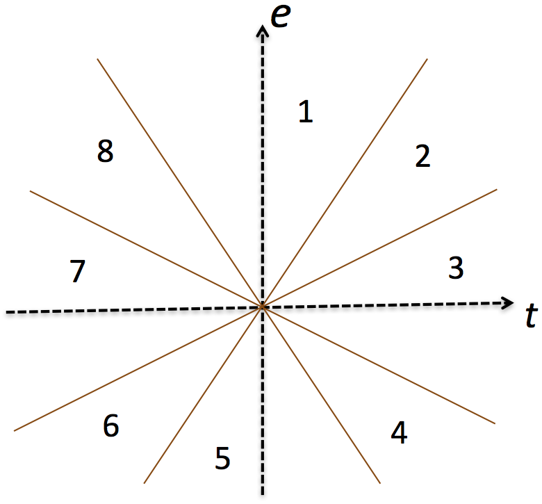
Figure 3: (color online) Adiabatic domains for the 4-state problem. There are 8 domains separated by 4 solid lines $e=(\pm b_{2}\pm b_{1})t$. We determine these lines from the condition that a pair of diabatic energy levels of $H(t,e)$ in Eq. (62) is degenerate, $E_{i}(t,e)=E_{j}(t,e)$. The time evolution is adiabatic at large $|\bm{x}|=\sqrt{t^{2}+e^{2}}$ in each domain away from its boundaries. WKB solutions in neighboring domains are connected via $2\times 2$ Landau-Zener scattering matrices. Here $b_{1}=1$ and $b_{2}=0.5$.

Let us explicate this picture for the 4-state model analyzed in the main text. To determine $\kappa^{ab}(\bm{x})$ and the adiabatic domains, we can use any of the Hamiltonians, $H_{0}(t,e)\equiv H(t,e)$ or $H_{1}(t,e)$. Take

$${H}(t,e)=\left(\begin{array}[]{cccc}b_{1}t+e&0&g&-\gamma\\ 0&-b_{1}t+e&\gamma&g\\ g&\gamma&b_{2}t&0\\ -\gamma&g&0&-b_{2}t\end{array}\right),$$ (62)

When $t$ and $e$ are large, the off-diagonal part of $H(t,e)$ is typically negligible. Then, the adiabatic and diabatic energy levels and eigenstates coincide. To the leading order, $\langle e_{a}(\bm{x})|\partial_{t}e_{b}(\bm{x})\rangle=0$, $p_{0}^{a}(\bm{x})-p_{0}^{b}(\bm{x})\to\infty$ and

$$\kappa^{ab}(\bm{x})=\frac{\langle e_{a}(\bm{x})|\partial_{t}e_{b}(\bm{x})\rangle}{p_{0}^{a}(\bm{x})-p_{0}^{b}(\bm{x})}=0,$$ (63)

i.e. the dynamics are purely adiabatic.

Adiabaticity breaks down when two of the diabatic energies $E_{1}=b_{1}t+e,E_{2}=-b_{1}t+e,E_{3}=b_{2}t$ and $E_{4}=-b_{2}t$ are close. Consider, for example, levels $E_{2}$ and $E_{3}$. First order perturbation theory in the off-diagonal part of $H(t,e)$ yields

$$\kappa^{23}(\bm{x})=\frac{\gamma(b_{1}+b_{2})}{(E_{3}-E_{2})^{3}}=\frac{\gamma(b_{1}+b_{2})}{[(b_{1}+b_{2})t-e]^{3}}.$$ (64)

The breakdown occurs near the line $e=(b_{1}+b_{2})t$ on which $E_{2}(t,e)=E_{3}(t,e)$. However, the nonadiabatic region where $\kappa^{23}(\bm{x})\geq 1$ is confined inside a small angle of order $1/t$, whose bisector is the $e=(b_{1}+b_{2})t$ line. Altogether equations $E_{1}(t,e)=E_{3}(t,e)$, $E_{1}(t,e)=E_{4}(t,e)$, $E_{2}(t,e)=E_{3}(t,e)$ and $E_{2}(t,e)=E_{4}(t,e)$ define four lines $e=(\pm b_{2}\pm b_{1})t$ in the coordinate space $(t,e)$. They divide the $(t,e)$ plane into eight adiabatic domains shown in Fig 3. The remaining two degeneracies $E_{1}(t,e)=E_{2}(t,e)$ and $E_{3}(t,e)=E_{4}(t,e)$ are insignificant, because these levels are not directly coupled to each other (matrix elements $H_{12}$ and $H_{34}$ are zero).

An important ingredient of the ordinary WKB method in quantum mechanics is the matching conditions near the turning points. In our multidimensional case, the hypersurfaces, where $\kappa^{ab}$ is large and the semiclassical approximation (57) breaks down, play the role of the turning points. In the 4-state example above these are the four lines where two of the diabatic levels are degenerate, see Fig 3. Similarly, in the driven generalized Tavis-Cummings model in the main text, the adiabaticity is violated when two levels get close. In cases like these, we obtain the matching (scattering) conditions by solving a 2$\times$2 scattering problem for these two states, say $a$ and $b$. The rest of the levels continue to evolve adiabatically, since they are well separated from levels $a$ and $b$ and from each other. Then, there is the following linear relationship between the semiclassical solutions (57) in neighboring domains $\alpha$ and $\beta$ separated by a hypersurface on which levels $a$ and $b$ are degenerate:

$$\Psi_{\alpha}^{c}=\sum_{d=a,b}S^{cd}_{\alpha\beta}\Psi_{\beta}^{d},\quad S_{\alpha\beta}=\bar{S}_{\alpha\beta;ab}\oplus\bar{I}_{ab},$$ (65)

where $c$ takes values $a$ and $b$, $\bar{S}_{\alpha\beta;ab}$ is a $2\times 2$ Landau-Zener scattering matrix for states $a$ and $b$ evaluated near the degeneracy hypersurface, and $\bar{I}_{ab}$ is a unit matrix acting on the remaining states.

We see that the zero curvature condition makes an explicit solution of the scattering problem possible in two ways. First, it allows us to choose a path ${\cal P}_{\infty}$ connecting the initial and final points that goes through a series of adiabatic domains at large $|\bm{x}|$. Second, in each such domain it facilitates a multidimensional WKB approach. Relatively simple scattering matrices connect WKB solutions in neighboring domains. In our examples, these were $2\times 2$ Landau-Zener matrices, but other solvable systems may have other matching conditions. We thus obtain the desired scattering matrix for the evolution from $t=-\infty$ to $t=+\infty$ by going sequentially from the domain that contains $t=-\infty$ to the one containing $t=+\infty$ always keeping $|\bm{x}|$ large and using Eqs. (57) and (65) along the way. For example, to determine the transition probabilities for $H(t,e)$ in Eq. (62), we need to go from domain #7 to domain #3 in Fig 3.

.2 Transition Probabilities for the 4-State Model: Direct Calculation

In this section, we detail the calculation of transition probabilities for the new 4-state model $h(\tau)$ [Eq. (16) in the main text]. In particular, we show how the phases accumulated during adiabatic evolution and Landau-Zener scattering in between adiabatic domains drop out from the final result.

Consider the case $v<b_{1}-b_{2}$ and the path ${\cal P}_{\infty}$ shown in Fig. 2(a) of the main text. This path goes from domain #7 to domain #3 in Fig 3. Its horizontal part crosses the four lines in Fig 3 where the adiabaticity is violated at points $t_{13},t_{14},t_{23}$ and $t_{24}$ marked with crosses in Fig. 2(a). The vertical piece of ${\cal P}_{\infty}$ does not contain points with nonadiabatic transitions. The evolution along this piece is adiabatic, described by Eq. (57), and does not affect the final transition probabilities.

Therefore, it is sufficient to consider only the horizontal part of ${\cal P}_{\infty}$. Evolution along this fragment occurs with the Hamiltonian (62), where $e=vR+e_{0}\gg e_{0},g,\gamma$. We show the adiabatic levels of this Hamiltonian in Fig. 4. Due to the large value of $e$, anticrossings are well separated in energy from the rest of the levels. The matrix of evolution along the horizontal piece of ${\cal P}_{\infty}$ is

$$\begin{split}{S}={U}^{t=R,t_{24}}{S}^{24}_{\mathrm{LZ}}{U}^{t_{24},t_{23}}{S}^{23}_{\mathrm{LZ}}{U}^{t_{23},t_{14}}\times\\ {S}^{14}_{\mathrm{LZ}}{U}^{t_{14},t_{13}}{S}^{13}_{\mathrm{LZ}}{U}^{t_{13},t=-R},\end{split}$$ (66)

where $4\times 4$ matrices ${U}^{\gamma,\delta}$ and ${S}^{ij}_{\mathrm{LZ}}$ represent the adiabatic evolution between the time moments $\gamma$ and $\delta$ on the path ${\cal P}_{\infty}$ and pairwise Landau-Zener transitions between states $i$ and $j$, respectively. The Landau-Zener amplitudes are known [see, e.g., Refs. 32-35 in the main text]. We have

$${S}^{13}_{\mathrm{LZ}}=\left(\begin{array}[]{cccc}\sqrt{p_{1}}&0&i\sqrt{q_{1}}e^{i\phi_{g}}&0\\ 0&1&0&0\\ i\sqrt{q_{1}}e^{-i\phi_{g}}&0&\sqrt{p_{1}}&0\\ 0&0&0&1\end{array}\right),$$ (71)

$${S}^{24}_{\mathrm{LZ}}=\left(\begin{array}[]{cccc}1&0&0&0\\ 0&\sqrt{p_{1}}&0&i\sqrt{q_{1}}e^{-i\phi_{g}}\\ 0&0&1&0\\ 0&i\sqrt{q_{1}}e^{i\phi_{g}}&0&\sqrt{p_{1}}\end{array}\right),$$ (76)

$${S}^{14}_{\mathrm{LZ}}=\left(\begin{array}[]{cccc}\sqrt{p_{2}}&0&0&-i\sqrt{q_{2}}e^{i\phi_{\gamma}}\\ 0&1&0&0\\ 0&0&1&0\\ -i\sqrt{q_{2}}e^{-i\phi_{\gamma}}&0&0&\sqrt{p_{2}}\end{array}\right),$$ (81)

$${S}^{23}_{\mathrm{LZ}}=\left(\begin{array}[]{cccc}1&0&0&0\\ 0&\sqrt{p_{2}}&i\sqrt{q_{2}}e^{-i\phi_{\gamma}}&0\\ 0&i\sqrt{q_{2}}e^{i\phi_{\gamma}}&\sqrt{p_{2}}&0\\ 0&0&0&1\end{array}\right).$$ (86)

Here

$$p_{1}=e^{-2\pi g^{2}/(b_{1}-b_{2})},\,\,\,p_{2}=e^{-2\pi\gamma^{2}/(b_{1}+b_{2})},\,\,\,q_{1,2}=1-p_{1,2},$$

and $\phi_{g}$, $\phi_{\gamma}$ are transition phases associated with couplings $g$ and $\gamma$ in Eq. (62), respectively. The sign in front of $\phi_{g,\gamma}$ depends on which level has a higher slope at the crossing of the corresponding diabatic levels. Amplitudes associated with the couplings $-\gamma$ in Eq. (62) acquire additional minus signs in $S_{\mathrm{LZ}}^{14}$.

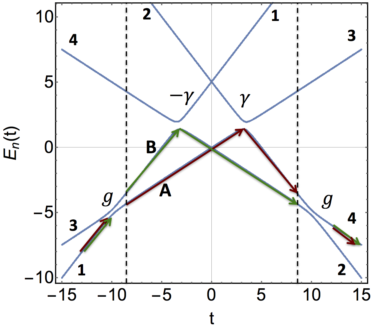
Figure 4: (color online) Energies of the Hamiltonian (62) as functions of $t$ (adiabatic levels). Numbers 1 through 4 indicate diabatic levels. For each avoided crossings we display the corresponding pairwise coupling $g$ or $\pm\gamma$. Red and green arrows show the two trajectories $A$ and $B$ that contribute to the amplitude of the transition from diabatic level 1 to level 4. In the time interval between vertical dashed lines these trajectories have different dynamical phases. Here $b_{1}=1,b_{2}=.5,e=5.0,g=0.2$, and $\gamma=0.3$.

Let us, for example, evaluate the level 1 to level 4 transition amplitude $S_{1\rightarrow 4}$, i.e. the matrix element $S_{14}$ of Eq. (66). We work in the diabatic basis. As mentioned in the previous section, far away from avoided crossings diabatic and adiabatic bases coincide, i.e. matrices $U^{\gamma,\delta}$ in Eq. (66) are diagonal. It follows from Eq. (66) that there are two “trajectories” that contribute to this amplitude – shown with green and red arrows and marked as A and B in Fig. 4, i.e.

$$S_{1\rightarrow 4}=S^{A}+S^{B}.$$ (87)

The adiabatic (dynamical) phases accumulated on these trajectories are

$$\phi_{d}=-\int_{-R}^{R}E(t)\,dt,$$ (88)

which are the areas under the curves $A$ and $B$ in Fig. 4. In order to make these phases well-defined, we use a convention that a trajectory jumps from one adiabatic level to another as the result Landau-Zener tunneling at the moment of the minimal separation between the levels. Due to the symmetry of the spectrum of the Hamiltonian (62) under the reflection $t\rightarrow-t$, areas under the curves $A$ and $B$ are the same, i.e. $\phi_{d}^{A}=\phi_{d}^{B}\equiv\phi_{d}$. This is true even though at intermediate times between vertical dashed lines in Fig. 4, the adiabatic phases of trajectories $A$ and $B$ are different.

Thus, using also the above expressions for the scattering matrices ${S}^{ij}_{\mathrm{LZ}}$, we get

$$S^{\rm A} = e^{i\phi_{d}}(i\sqrt{q_{1}}e^{i\phi_{g}})(i\sqrt{q_{2}}e^{-i\phi_{\gamma}})(i\sqrt{q_{1}}e^{-i\phi_{g}}),$$ (89)

$$S^{\rm B} = e^{i\phi_{d}}(\sqrt{p_{1}})(-i\sqrt{q_{2}}e^{-i\phi_{\gamma}})(\sqrt{p_{1}}),$$ (90)

$$S_{1\rightarrow 4}=S^{\rm A}+S^{\rm B}=-ie^{i(\phi_{d}-\phi_{\gamma})}\sqrt{q_{2}},$$ (91)

and the corresponding transition probability,

$$P_{1\rightarrow 4}=|S_{1\rightarrow 4}|^{2}=q_{2}.$$ (92)

We see that both dynamic $\phi_{d}$ and Landau-Zener $\phi_{g}$ and $\phi_{\gamma}$ phases drop out from the final answer for the transition probability. Note, however, that interference between the semiclassical trajectories $A$ and $B$ does take place despite this cancellation, $|S_{1\rightarrow 4}|^{2}\neq|S^{\rm A}|^{2}+|S^{\rm B}|^{2}$. For example, interference is responsible for the independence of the final probability (92) from the coupling $g$, even though avoided crossings with this coupling occur for both contributing trajectories.

Similarly, dynamical phases (88) as well as $\phi_{\gamma}$ and $\phi_{g}$ cancel out from all transition probabilities due to the reflection symmetry in the spectra of ${H}_{0}$ and ${H}_{1}$. Therefore, as long as we are interested in the transition probabilities only, we can disregard the matrices ${U}^{\alpha,\beta}$ in (66) and set the Landau-Zener phases $\phi_{g,\gamma}$ in the scattering matrices ${S}^{ij}_{\mathrm{LZ}}$ to zero. The calculation of ${S}$ then reduces to finding a properly ordered product of such truncated scattering matrices ${S}^{ij}_{\mathrm{LZ}}$.