Chameleon Field Dynamics During Inflation

Abstract

By studying the chameleon model during inflation, we investigate whether it can be a successful inflationary model, wherein we employ the common typical potential usually used in the literature. Thus, in the context of the slow–roll approximations, we obtain the number of e–folding for the model to verify the ability of resolving the problems of standard big bang cosmology. Meanwhile, we apply the constraints on the form of the chosen potential and also on the equation of state parameter coupled to the scalar field. However, the results of the present analysis show that there is not much chance of having the chameleonic inflation. Hence, we suggest that if through some mechanism the chameleon model can be reduced to the standard inflationary model, then it may cover the whole era of the universe from the inflation up to the late time.

PACS numbers: 04.50.Kd, 98.80.-k, 98.80.Cq, 95.36.+x
Keywords: Chameleon Cosmology; Inflationary Universe; Slow–Role Approximations.

1 Introduction

The recent accelerated expansion of the universe has been reported by the various observed cosmological data such as the luminosity redshift relation for the supernovae type Ia (SNIa) [1]–[4], the large scale structure formation [5], the baryon acoustic oscillation (BAO) [6, 7], and the cosmic microwave background (CMB) temperature anisotropies measured by some experiments such as COBE [8], WMAP [9]–[12] and Planck [13]–[15]. Numerous attempts have been proposed to present a theoretical explanation to this mysterious acceleration of the universe, which could have arisen from a dark energy component or being due to departure of gravity from general relativity on cosmological scales, see, e.g., Refs. [16]–[26]. In the former mechanism, dark energy is “some kind of matter” with a negative pressure that is supposed to be responsible for the accelerated expansion of the universe. However, the important point is that the parameters entering each mechanism must satisfy both the current astronomical observations and the laboratory experiments.

Amongst different models for dark energy, the cosmological constant is the simplest one in which its energy density is constant. As this model has some difficulties, such as the cosmological constant problem [27]–[33] and the coincidence problem [29, 30, 33], scalar fields have been introduced as dark energy component with a dynamical equation of state, see, e.g., Refs. [34]–[39]. Essentially, scalar fields have long history in physics, and more recently, they have played an important role in both cosmology and particle physics. In fact, it is believed that our universe consists of some scalar fields in addition to the matter fields. In this context, the scalar–tensor theory of gravitation recently becomes one of the most popular alternatives¹ to the Einstein gravitational theory, see, e.g., Refs. [20, 41]–[43]. In particular, quintessence is a more general dynamical model in which the energy source of the universe, unlike the cosmological constant, varies in space and time [44]–[48].

On the other hand, the higher dimensional gravities, e.g. the string theory and supergravity, predict some massless scalar fields that couple directly to the matter with gravitational strength, see, e.g., Refs. [49, 50]. These theories may motivate ones to investigate the scalar–tensor theory wherein the scalar field couples to the matter with the gravitational strength. However, due to such coupling, a fifth force and also large violation of the equivalence principle (EP) should be detected [51, 52] in contrast to the results of the solar system tests of gravity [53]–[55]. Thus, if one considers such coupling to the matter for the quintessence field, then some mechanisms must effectively screen those resulted forces locally and also prevent the EP–violation. In fact, the notion of screening mechanisms is how a scalar field can act as dark energy on cosmological scales while being shielded in the regions of high density, such as on the earth (see, e.g., Refs. [56, 57] for a review on this issue). There are usually two main ways for having a suitable scalar field model while avoiding the EP–violation:

• Such a scalar field must usually be very light and its coupling to the matter should be tuned to extremely small values [58]–[60].

• The scalar field can couple to the matter fields with the gravitational strength and then, acquires a mass depending on the background matter density of the environment which leads its interaction to be effectively short–ranged [61]–[76].

In this regard, the chameleon model proposed in Refs. [61, 62] invokes a screening mechanism based on the second approach remaining consistent with the tests of gravity on the terrestrial and the solar system scales. Actually, in this type of chameleon cosmology, the corresponding scalar field couples to an ambient matter field through a conformal factor, relating the Jordan and Einstein frames, with the gravitational strength, and consequently, its mass is no longer fixed but depends on the environmental situations. In the dense environments, such as on the earth, the chameleon field acquires a large mass that makes its effects short–ranged, and hence, becomes invisible to be searched for the EP–violation and fifth force in the current experimental and observational tests. Such a property of the chameleon field is of great deal of importance. On the other hand, it is very light in diluted matter situations, such as the cosmological scales, and thus, the chameleon field may play the role of dark energy causing the cosmic late time acceleration.

However, under a very general conditions, there were proved two theorems by which it has been claimed that they limit a cosmological impact of the chameleon field [77, 78]. Actually, it was shown that at the present cosmological density the Compton wavelength of the chameleon field should be of the order of $1$ Mpc, and the conformal factor during the last Hubble time is almost a practically constant value. Their results imply that chameleon–like scalar fields have a negligible effect on density perturbations on linear scales,¹ and may not account for the observed cosmic acceleration except as some form of dark energy. Nevertheless, it has been indicated [79] that even if the cosmological factor being in principle constant during the last Hubble time, this will not prevent for the chameleon field to be responsible for a late–time acceleration of the universe expansion. Indeed, the conformal factor describing the interaction of the chameleon field with an ambient matter may lead to deviations of the matter and radiation densities in the universe from their canonical forms $1/a^{3}$ and $1/a^{4}$, where $a$ is the cosmological factor describing a dynamics of the universe expansion. However, one may assert that these results in [79] are model–independent, since the shape of the potential of the self–interaction of the chameleon field was not specified. In addition, it has been shown [80] that the cosmological constant and dark energy density might be induced by torsion in the Einstein–Cartan gravitational theory. Actually, as torsion is a natural geometrical quantity additional to the metric tensor, the analysis of the nature of the cosmological constant performed in [80] provides a robust geometrical background for the origin of the cosmological constant and dark energy density.

In the present work, we propose to study the chameleonic behavior during another important acceleration era, namely the inflation which is an extremely rapid expansion that resolves some important problems of the standard cosmological model such as the flatness, horizon and monopole [81]–[91]. By this paper, we aim to investigate whether the chameleon model is a successful model during the inflation, and what would be the ambient matter of the universe during the inflation that the chameleon field is coupled to. In this case, one may claim that the chameleon field, as a single scalar field, being responsible for the acceleration of the universe both at the very early and at the late time. To perform this task, we consider a coupling between the chameleon scalar field and an unknown matter scalar field with the equation of state parameter $w$. In addition, to probe the behavior of the model in the inflationary era, we expect to specify the value of $w$ via the constraints during the analysis of the results in order to figure out the type of this unknown coupled matter field.

Moreover, the possibility of describing the chameleon and the inflaton by one single scalar field has also been investigated in Ref. [92] where the scenario is based on a modified supersymmetric potential introduced by Kachru, Kallosh, Linde and Trivedi (KKLT) [93]. Indeed, by using this modified construction of KKLT potential, they have attempted to embed the chameleon scenario within the string compactifications, where it has been shown that the volume modulus of the compactification can act as a chameleon field. The late time investigation has been presented in Ref. [94], while Ref. [92] describes the scenario during the inflation wherein it has been presented that in order to cover the cosmology of both the late time and the very early universe, there exists a superpotential consisting of two pieces, which one drives the inflation in the very early universe, and the other one is responsible for the chameleon screening at the late time.

The work is organized as follows. In the next section, we introduce the model and obtain the field equations of motion by taking the variation of the action. In Sect. $3$, we investigate the model during the inflation by imposing the slow–roll approximations. Also, we compute the value of e–folding number of the model for the common typical potential usually used in the context of the chameleon theory in the literature, and then, set the constraints to pin down the free parameters of the model. Finally, we conclude the work in Sect. $4$ with the summary of our results.

2 Chameleon Scalar Field Model

We start with the following known action that governs the dynamics of the chameleon scalar field model in 4–dimensions, i.e.

$$S\!\!\! =\!\!\! \!\!\int{\rm d}^{4}x\sqrt{-g}\left[\frac{M^{2}_{\rm Pl}R}{2}\!-\!\frac{1}{2}\partial_{\mu}\phi\partial^{\mu}\phi-V(\phi)\right]$$ (1)

$$+\sum_{i}\int{\rm d}^{4}x\sqrt{-{\tilde{g}}^{(i)}}{L_{\rm m}^{(i)}}\left({\psi}^{(i)},{\tilde{g}}^{(i)}_{\mu\nu}\right),$$

where $R$ is the Ricci scalar constructed from the metric $g_{\mu\nu}$ with signature $(-,+,+,+)$, $g$ is the determinant of the metric, $M_{\rm Pl}\equiv(8\pi G)^{-1/2}\approx 10^{27}eV$ is the reduced Planck mass (we use the units in which $c=1=\hbar$) and the lowercase Greek indices run from zero to three. Also, $\phi$ is a scalar field, $V(\phi)$ is a self–interacting potential, $L_{\rm m}^{(i)}$’s are the Lagrangians of the matter fields, $\psi^{(i)}$’s are various matter scalar fields, $\tilde{g}_{\mu\nu}^{(i)}$’s are the matter field metrics that are conformally related to the Einstein frame metric $g_{\mu\nu}$ via

$${\tilde{g}}^{(i)}_{\mu\nu}={e}^{{2\frac{{\beta}_{i}\phi}{M_{\rm Pl}}}}{g}_{\mu\nu},$$ (2)

where $\beta_{i}$’s are dimensionless constants representing different non–minimal coupling constant between the scalar field and each matter species. However, in our analysis, we just focus on a single matter component, and henceforth, we drop the index $i$. We also consider the universe to be described by the spatially flat Friedmann–Lemaître–Robertson–Walker (FLRW) metric in the Einstein frame as

$$ds^{2}=-dt^{2}+a^{2}(t)\left(dx^{2}+dy^{2}+dz^{2}\right),$$ (3)

where $t$ is the cosmic time. Obviously, the corresponding metric in the Jordan frame is

$$d\tilde{s}^{2}=-{e}^{{2\frac{{\beta}\phi}{M_{\rm Pl}}}}dt^{2}+\tilde{a}^{2}(t)\left(dx^{2}+dy^{2}+dz^{2}\right),$$ (4)

where $\tilde{a}(t)$ is the scale factor in the Jordan frame, i.e. $\tilde{a}(t)\equiv a(t)\exp({\beta\phi/M_{\rm Pl}})$.

Varying the action with respect to the scalar field yields the field equation of motion

$$\Box\phi=V^{\prime}(\phi)-\frac{{\beta}}{M_{\rm Pl}}e^{4\frac{{\beta}\phi}{{M}_{\rm Pl}}}{\tilde{g}}^{\mu\nu}{\tilde{T}}_{\mu\nu},$$ (5)

where $\Box\equiv\nabla^{\alpha}\nabla_{\alpha}$ corresponding to the metric $g_{\mu\nu}$, the prime is the derivative with respect to the argument and $\tilde{T}_{\mu\nu}=-(2/\sqrt{-\tilde{g}})\delta(\sqrt{-\tilde{g}}L_{\rm m})/\delta{\tilde{g}}^{\mu\nu}$ is the energy–momentum tensor that is conserved in the Jordan frame, i.e. $\tilde{\nabla}_{\mu}{\tilde{T}^{\mu\nu}}=0$. We assume an unknown matter field as a perfect fluid with the equation of state $\tilde{p}=w\tilde{\rho}$ that, in the FLRW background, one has

$${\tilde{g}}^{\mu\nu}\tilde{T}_{\mu\nu}=-(1-3w)\tilde{\rho},$$ (6)

where $\tilde{\rho}$ is the matter density in the Jordan frame. As $\tilde{\rho}$ is not conserved in the Einstein frame, we propose to have a conserved matter density with the same equation of state, which is independent of $\phi$ and obeys the following relation in the Einstein frame

$$\rho\propto a^{-3(1+w)}.$$ (7)

In this respect, as the continuity equation for $\tilde{\rho}$ in the Jordan frame is

$$\dot{\tilde{\rho}}+3\frac{\dot{\tilde{a}}}{\tilde{a}}(1+w)\tilde{\rho}=0,$$ (8)

that yields $\left(\tilde{a}^{3(1+w)}\tilde{\rho}\right)_{,0}=0$, hence in order to have relation (7), one can define the conserved matter density in the Einstein frame as

$$\rho\equiv e^{3(1+w)\frac{{\beta}\phi}{M_{\rm Pl}}}\tilde{\rho}.$$ (9)

Therefore, equation (5) reads¹

$$\Box\phi=V^{\prime}(\phi)+(1-3w)\frac{\beta}{{M}_{\rm Pl}}\rho e^{(1-3w)\frac{{\beta}\phi}{M_{\rm Pl}}},$$ (10)

and thus, the dynamic of the scalar field is actually governed by an effective potential, i.e.

$$\Box\phi=V^{\prime}_{\rm eff}(\phi),$$ (11)

where

$${V}_{\rm eff}(\phi)\equiv V(\phi)+\rho(t)\,e^{(1-3w)\frac{\beta\phi}{M_{\rm Pl}}}.$$ (12)

As it is obvious, the effective potential depends on the background matter density $\rho$ of the environment. Consequently, the value of $\phi$ at the minimum of $V_{\rm eff}$ and the mass fluctuation about the minimum,² depend on the matter density. For instance, if one considers $V(\phi)$ as a decreasing function of $\phi$, while $\beta>0$ and $1-3w>0$, the minimum of the effective potential decreases by increasing $\rho$, hence, the mass of the scalar field will increase in a way that the chameleon field can be hidden from the local experiments.

By the FLRW metric (3), the field equation (11) gives the corresponding Klein–Gordon equation

$$\ddot{\phi}+3H\dot{\phi}+V^{\prime}_{\rm eff}(\phi)=0,$$ (13)

where $H(t)\equiv\dot{a}/a$ is the Hubble expansion rate of the universe, dot denotes the derivative with respect to the cosmic time, and the scalar field is only a function of the time due to the homogeneity and isotropy. In addition, one can obtain the Friedmann–like equations for the model by the variation of the action with respect to the metric $g_{\mu\nu}$ in the context of the perfect fluid as

$$3M^{2}_{\rm Pl}H^{2}=\frac{1}{2}\dot{\phi}^{2}+V_{\rm eff}(\phi)$$ (14)

and

$$2\frac{\ddot{a}}{a}+H^{2}=-\frac{1}{M^{2}_{\rm Pl}}\left[\frac{1}{2}\dot{\phi}^{2}-V(\phi)+w\rho e^{\left(1-3w\right)\frac{\beta\phi}{M_{\rm Pl}}}\right].$$ (15)

And in turn, the time derivative of the Hubble parameter, that will be needed later on, is

$$M^{2}_{\rm Pl}\dot{H}=-\frac{1}{2}\dot{\phi}^{2}-\frac{1}{2}(1+w)\rho e^{\left(1-3w\right)\frac{\beta\phi}{M_{\rm Pl}}}.$$ (16)

Now, in the following section, we mainly consider these equations of motion in the inflationary era.

3 Chameleon During Inflation

In this section, by applying the common typical chameleonic potential, we propose to investigate the chameleon model during the inflation while considering a non–minimal coupling between the chameleon field and an unknown matter scalar field with the equation of state parameter $w$ which one may expect to be specified via the constraints during the analysis. It is remarkable that the chameleon field does not couple to the radiation (with $w=1/3$) as the trace of its energy–momentum tensor is zero.

In this context, a potential, that has mostly been considered in the literature, is in the form of inverse power–law [61]–[64], although a $\phi^{4}$ potential has also been investigated [63]. To cover all these kind of potentials, we consider it to be in general form

$$V(\phi)=\lambda M^{4}\left(M/\phi\right)^{n},$$ (17)

where $\lambda>0$ is a constant, $M$ is some mass scale and $n$ is a positive or negative integer constant (however, see the point below relation (43)). Furthermore, when $n\neq-4$, $M$ can be scaled such that, without loss of generality, one can set $\lambda$ equals to unity (although, we have kept it), whereas for $n=-4$, $M$ drops out and the $\phi^{4}$ theory is resulted [65, 67, 75, 76].

On the other hand, a successful inflationary model should resolve the puzzling issues of the standard big bang cosmology such as the flatness, horizon and monopole problems. In fact, an extremely rapid expansion would cause the homogeneity and isotropy of the universe at large scales. Amongst the mentioned difficulties, the horizon problem is more important than the others, for its resolution makes the other problems being solved automatically [95]. Thus, to check whether the model solves the mentioned problems, one should find the e–folding number, where it is believed that a viable inflationary model requires that the universe inflates by at least $50$ to $60$ times [96], or even more (i.e., nearly $70$ times or higher). In addition, we assume that the value of the effective potential being almost constant, i.e. almost being equivalent to a quasi de Sitter expansion, then, we can obtain the number of e–folding by imposing the slow–roll conditions for the model as the most inflationary models are built upon the slow–roll approximations.

In this respect, we use the Hubble slow–roll parameters defined as¹

$$\epsilon\equiv-\frac{\dot{H}}{H^{2}}\qquad\qquad{\rm and}\qquad\qquad\eta\equiv-\frac{|\ddot{\phi}|}{H|\dot{\phi}|}.$$ (18)

Now, during the inflation, to have an accelerated expansion of the scale factor (i.e., $\ddot{a}>0$) and a sufficiently long enough inflation (in order to solve the horizon problem), the slow–roll parameters must be very smaller than unity, i.e., $\epsilon\ll 1$ and $|\eta|\ll 1$ [90, 95], that lead to the following two slow–roll conditions

$$\dot{\phi}^{2}\ll|V-\frac{1+3w}{2}\rho e^{(1-3w)\frac{\beta\phi}{M_{\rm Pl}}}|\qquad\qquad{\rm and}\qquad\qquad|\ddot{\phi}|\ll H|\dot{\phi}|,$$ (19)

where the first one is obtained by substituting equations (14) and (16) into definition $\epsilon$, and guaranties slowly rolling of the scalar field during the inflation. Note that, this condition is different from the corresponding one in the standard model due to the non–minimal coupling term. Under these slow–roll conditions, equations (13), (14) and (15) reduce to

$$\dot{\phi}\approx-\frac{1}{3H}V^{\prime}_{\rm eff}(\phi),$$ (20)

$$H^{2}\approx\frac{1}{3M^{2}_{\rm Pl}}V_{\rm eff}(\phi)$$ (21)

and

$$2\frac{\ddot{a}}{a}+H^{2}\approx-\frac{1}{M^{2}_{\rm Pl}}\left[-V(\phi)+w\rho e^{\left(1-3w\right)\frac{\beta\phi}{M_{\rm Pl}}}\right].$$ (22)

Thus, the slow–roll parameters (18) themselves read

$$\epsilon\approx\epsilon_{1}+\frac{3(1+w)\rho e^{\left(1-3w\right)\frac{\beta\phi}{M_{\rm Pl}}}}{2V_{\rm eff}(\phi)}$$ (23)

and

$$\eta\approx\eta_{1}-\epsilon+\frac{3(1+w)(1-3w)\beta\rho e^{\left(1-3w\right)\frac{\beta\phi}{M_{\rm Pl}}}}{M_{\rm Pl}V^{\prime}_{\rm eff}(\phi)},$$ (24)

where the first relation is obtained using equations (16), (20) and (21), and the second one yields through taking the time derivative of equation (20), then employing equations (20) and (21) wherein considering the matter density conservation in the Einstein frame, i.e. $\dot{\rho}=-3H(1+w)\rho$. Also, in the same analogy with the standard model [90, 95], we have defined $\epsilon_{1}$ and $\eta_{1}$ as

$$\epsilon_{1}\equiv\frac{M^{2}_{\rm Pl}}{2}\left(\frac{V^{\prime}_{\rm eff}(\phi)}{V_{\rm eff}(\phi)}\right)^{2}$$ (25)

and

$$\eta_{1}\equiv M^{2}_{\rm Pl}\frac{V^{\prime\prime}_{\rm eff}(\phi)}{V_{\rm eff}(\phi)}.$$ (26)

However, due to the presence of the matter field, the slow–roll parameters are different from the standard model. Now, substituting potential (17) into equation (23) leads to

$$\epsilon\approx\frac{M^{2}_{\rm Pl}}{2}\left[\frac{-n\frac{\lambda M^{4+n}}{\phi^{n+1}}+\frac{\left(1-3w\right)\beta}{M_{\rm Pl}}\rho e^{\frac{\left(1-3w\right)\beta\phi}{M_{\rm Pl}}}}{\frac{\lambda M^{4+n}}{\phi^{n}}+\rho e^{\frac{\left(1-3w\right)\beta\phi}{M_{\rm Pl}}}}\right]^{2}+\frac{3}{2}\left[\frac{(1+w)\rho e^{\left(1-3w\right)\frac{\beta\phi}{M_{\rm Pl}}}}{\frac{\lambda M^{4+n}}{\phi^{n}}+\rho e^{\frac{\left(1-3w\right)\beta\phi}{M_{\rm Pl}}}}\right].$$ (27)

As mentioned earlier, in order to check the model during the inflation, one needs to obtain the number of e–folding that somehow describes the rate of the expansion, and is defined as

$$N=\int_{t_{i}}^{t_{e}}Hdt=\int_{\phi_{i}}^{\phi_{e}}\frac{H}{\dot{\phi}}d\phi,$$ (28)

where the subscripts “i” and “e” denote the beginning and the end of the inflation, respectively. By using equations (20) and (21), we can easily get

$$N\!\!\!\!\!\! \approx\!\!\!\! \!\!\!-\frac{1}{M^{2}_{\rm Pl}}\int_{\phi_{i}}^{\phi_{e}}\frac{V_{\rm eff}(\phi)}{V^{\prime}_{\rm eff}(\phi)}d\phi$$ (29)

$$= \!\!\!-\frac{1}{M^{2}_{\rm Pl}}\int_{\phi_{i}}^{\phi_{e}}\frac{\frac{\lambda M^{4+n}}{\phi^{n}}+\rho e^{\frac{\left(1-3w\right)\beta\phi}{M_{\rm Pl}}}}{-n\frac{\lambda M^{4+n}}{\phi^{n+1}}+\frac{\left(1-3w\right)\beta}{M_{\rm Pl}}\rho e^{\frac{\left(1-3w\right)\beta\phi}{M_{\rm Pl}}}}d\phi,$$

where the last line is obtained by substituting potential (17) into the effective potential and its derivative. In addition to the number of free parameters used in this integral, we are supposed to evaluate it for the model in hand that makes it not to be solved easily as it stands. In other words, although $\rho$ is independent of $\phi$, both of them are engaged through the equations of motion.

Hence, while using the corresponding equations of the model, we proceed by indicating the coupling term $\rho\,\exp{\left[(1-3w)\beta\phi/M_{\rm Pl}\right]}$ in terms of $\phi$ alone. To perform this task, we start from relation (24) and rewrite it as

$$\ddot{\phi}+(\eta_{1}-\epsilon)H\dot{\phi}-\frac{(1+w)(1-3w)\beta\rho e^{\left(1-3w\right)\frac{\beta\phi}{M_{\rm Pl}}}}{M_{\rm Pl}}\approx 0.$$ (30)

According to Ref. [64], the chameleon is slow rolling along the minimum of the effective potential and hence, follows the attractor solution $\phi\approx\phi_{\rm min}$ as long as $m_{\phi}\gg H$. Such a condition, using equation (21) and definition $m^{2}_{\phi}=V^{\prime\prime}_{\rm eff}(\phi_{\rm min})$, leads to $\eta_{1}\gg 1$.¹ Hence, by considering it into relation (30), one can neglect $\epsilon$ with respect to $\eta_{1}$, and in turn, neglects the term $\ddot{\phi}$ with respect to $\eta_{1}H\dot{\phi}$ term due to condition (19). Therefore, relation (30) reads

$$\eta_{1}H\dot{\phi}-\frac{(1+w)(1-3w)\beta\rho e^{\left(1-3w\right)\frac{\beta\phi}{M_{\rm Pl}}}}{M_{\rm Pl}}\approx 0.$$ (31)

At this stage, by substituting definition (26) and equations (20) and (21) into relation (31), and performing some manipulations, it yields

$$\frac{(1-3w)\beta}{M_{\rm Pl}}A\rho^{2}e^{2\left(1-3w\right)\frac{\beta\phi}{M_{\rm Pl}}}\!+\!\frac{(1-3w)\beta}{M_{\rm Pl}}B_{+}(\phi)\rho e^{\left(1-3w\right)\frac{\beta\phi}{M_{\rm Pl}}}+V^{\prime}V^{\prime\prime}\approx 0.$$ (32)

Then, by considering $w\neq 1/3$, the following two solutions corresponding to positive and negative parts are obtained as

$$\rho e^{\left(1-3w\right)\frac{\beta\phi}{M_{\rm Pl}}}\approx\frac{-B_{+}(\phi)\pm\sqrt{B_{-}(\phi)^{2}+C(\phi)}}{2A},$$ (33)

where

$$A\!\!\! \equiv\!\!\! \frac{1}{M^{2}_{\rm Pl}}\left[(1-3w)^{2}\beta^{2}+3(1+w)\right],$$

$$B_{\pm}(\phi)\!\!\! \equiv\!\!\! V^{\prime\prime}\pm\frac{(1-3w)\beta}{M_{\rm Pl}}V^{\prime}+\frac{3(1+w)}{M^{2}_{\rm Pl}}V,$$

$$C(\phi)\!\!\! \equiv\!\!\! \frac{12(1-3w)(1+w)\beta}{M_{\rm Pl}}V^{\prime}\left[\frac{V}{M^{2}_{\rm Pl}}-\frac{V^{\prime\prime}}{(1-3w)^{2}\beta^{2}}\right].$$ (34)

By employing the typical potential (17), the last two definitions can be rewritten as

$$B_{\pm}(\phi)=\frac{\lambda M^{4+n}}{\phi^{n}}B^{*}_{\pm}(\phi),$$

$$C(\phi)=\frac{\lambda^{2}M^{2(4+n)}}{\phi^{2n}}C^{*}(\phi)$$ (35)

and thus, relation (33) is

$$\rho e^{\left(1-3w\right)\frac{\beta\phi}{M_{\rm Pl}}}\approx\frac{\lambda M^{4+n}}{\phi^{n}}F^{(\pm)}(\phi)=V(\phi)F^{(\pm)}(\phi),$$ (36)

where $F^{(\pm)}$ correspond to positive and negative parts of the solutions, and are defined as

$$F^{(\pm)}(\phi)\equiv\frac{-B^{*}_{+}(\phi)\pm\sqrt{B^{*\,2}_{-}(\phi)+C^{*}(\phi)}}{2A},$$ (37)

in which

$$B^{*}_{\pm}(\phi)\!\!\! \equiv\!\!\! \frac{n(n+1)}{\phi^{2}}\mp n\frac{(1-3w)\beta}{M_{\rm Pl}\phi}+\frac{3(1+w)}{M^{2}_{\rm Pl}},$$

$$C^{*}(\phi)\!\!\! \equiv\!\!\! -\frac{12n(1-3w)(1+w)\beta}{M_{\rm Pl}}\left[\frac{1}{{M^{2}_{\rm Pl}}\phi}-\frac{n(n+1)}{(1-3w)^{2}\beta^{2}\phi^{3}}\right].$$ (38)

In fact, through the chameleon condition and some plausible approximations, relation (36) indicates that the coupling term $\rho\,\exp{\left[(1-3w)\beta\phi/M_{\rm Pl}\right]}$ has been taken to be proportional to $V(\phi)$, which leads to somehow relating the matter density as a function of the scalar field. However, on the other point of view, we are actually proceeding the work, as if one just continues the work by imposing relation (36) as a priori assumption. Moreover, using this relation results in the elimination of the free parameters $M$ and $\lambda$ in the subsequent calculations.

Now, let us substitute relations (36) into (27) and (29) to get

$$\epsilon^{(\pm)}(\phi)\approx\frac{M^{2}_{\rm Pl}}{2}\left[\frac{\frac{-n}{\phi}+\frac{(1-3w)\beta}{M_{\rm Pl}}F^{(\pm)}(\phi)}{1+F^{(\pm)}(\phi)}\right]^{2}+\frac{3}{2}\left[\frac{(1+w)F^{(\pm)}(\phi)}{1+F^{(\pm)}(\phi)}\right]$$ (39)

and

$$N^{(\pm)}(\phi)\approx-\frac{1}{M^{2}_{\rm Pl}}\int_{\phi_{i}}^{\phi_{e}}\frac{1+F^{(\pm)}(\phi)}{\frac{-n}{\phi}+\frac{(1-3w)\beta}{M_{\rm Pl}}F^{(\pm)}(\phi)}d\phi,$$ (40)

where $\epsilon^{(\pm)}(\phi)$ and $N^{(\pm)}(\phi)$ correspond to two different values of $F^{(\pm)}(\phi)$ defined in (37). Furthermore, in order to get the value of $\phi$ at the end of the inflation, we use the known relation

$$\epsilon|_{\phi=\phi_{e}}\approx 1,$$ (41)

that means the inflation ends when the slow–roll scenario breaks down by growing $\epsilon$ up to the order of one. Moreover, for indicating the value of $\phi_{i}$ at the beginning of inflation, we employ¹ [90, 102] the relation

$$r\approx 16\epsilon|_{\phi=\phi_{i}},$$ (42)

where the parameter $r$ is the ratio of the tensor perturbation amplitude to the scalar perturbation amplitude. The Planck temperature anisotropy measurements have released an upper limit for this parameter to be $r<0.11$ in $95\%$ confidence level [13]–[15].

Then, by using relations (39), (41) and (42), one can obtain the values of $\phi$ at the beginning and at the end of inflation, therefore the number of e–folding can be estimated numerically solving integral (40).² Through this analysis, we not only investigate the viability of the model by indicating the admissible number of e–folding, but also, we attempt to set constraints to pin down the free parameters of the model. As mentioned, the integral $N$ consists of many free parameters and hence, not easy to be solved analytically. In this regard, in what follows, through some values of $\beta$, $n$, $w$ and $r$, we estimate the integral numerically to attain admissible values for the number of e–folding. We work in an appropriate unit to set $M_{\rm Pl}=1$. Also, for choosing plausible values of $\beta$, we have noted that Weltman and Khoury, in their original suggestion for the chameleon model [61, 62], considered the possibility of coupling the scalar field to the matter field with the gravitational strength, and have shown that the chameleon theory is compatible while the coupling constant, $\beta$, is of the order of unity. However, Mota and Shaw have shown that the scalar field theories, which couple to the matter field much more strongly than gravity, are viable due to the non–linearity effects of the theory [65, 67]. Thus, we assume $\beta=0.1$, $1$ and $1000$ to cover more possible coupling strength. In addition, by taking $r=0.109$, $-1\leqslant w\leqslant 1$ and different values of $n$, we estimate the number of e–folding for these values of $\beta$. In this respect, and in the first step, we have depicted the behavior of e–folding $N$ with respect to $n$ and $w$ in Figs. $1$ and $2$. For example, for $\beta=1$, we illustrate the behavior of $N^{(-)}$ with respect to $n$ for some fixed values of $w$ with few plots in Fig. $1$, and also with respect to $w$ for some fixed values of $n$ with few plots in Fig. $2$. The results indicate that the power–law potentials with $n<0$, as a chameleon self–interacting potential (except $n=-2$ and odd–negative integers), with the equation of state parameters near $-1$ for the coupled matter field seem to be more compatible with the inflation. In Fig. $2$, the singularities around $w\approx 1/3$ are due to the fact that the chameleon field does not couple to the radiation. Also note that, the plots in Fig. $1$ have been drawn for the continuous range of parameter $n$ whereas we have assumed $n$ to be integer for the typical potential of the model. In order to attain an admissible number of e–folding more precisely, we calculate the two solutions $N^{(\pm)}$ for different chosen values of the free parameters $n$, $w$ and $\beta$. The results have been collected in Tables $1$–$5$, which indicate that for having a viable inflationary model, the self–interacting potential in the form of power–law with $n=-2$ and the equation of state parameter of the coupled field with $w=-1$ seems to be more appropriate than the other choices. However, the case $n=-2$ is not suitable as a chameleonic potential because it is linear and does not enable the model to be screened [75, 76]. Note that, the range of allowable $w$ tends to be larger for strongly coupling case (i.e., $\beta=1000$) than the other cases.

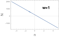
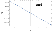
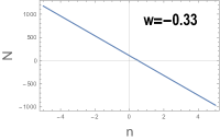
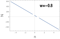
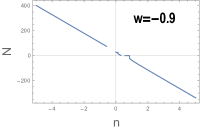
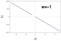
Figure 1: The figures show the behavior of e–folding $N^{(-)}$ with respect to $n$ for different values of $w$. As seen, the power–law potentials with $n<0$, as a self–interacting potential, with the equation of state parameters near $-1$ for the coupled matter field seem to be more suitable during the inflation. Also, we have set $\beta=1$, $r=0.109$ and $M_{\rm Pl}=1$ in an appropriate unit.

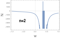
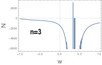
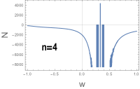
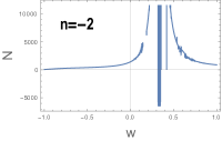
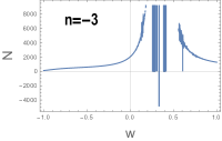
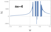
Figure 2: The figures show the behavior of e–folding $N^{(-)}$ with respect to the equation of state parameter of the coupled matter field $w$ for some different values of $n$. As seen, the power–law potentials with $n<0$, as a self–interacting potential, with the equation of state parameters near $-1$ for the coupled matter field seem to be more suitable during the inflation. Since the chameleon field does not directly couple to the radiation, the plots show some singularities near $w\approx 1/3$. Also, we have set $\beta=1$, $r=0.109$ and $M_{\rm Pl}=1$ in an appropriate unit.

Furthermore, there is another constraint in the chameleon model, i.e., $\beta V^{\prime}(\phi_{\rm min})<0$ as mentioned, e.g., in Refs. [61, 67]. It has been obtained due to $V^{\prime}_{\rm eff}(\phi_{\rm min})\approx 0$ that leads to

$$\phi_{\rm min}\approx\left[\frac{n\lambda M^{4+n}M_{\rm Pl}}{(1-3w)\beta\rho e^{(1-3w)\frac{\beta\phi_{\rm min}}{M_{\rm Pl}}}}\right]^{\frac{1}{n+1}}.$$ (43)

This relation implies that, if $\beta<0$, then $n$ can be either a negative integer or an even–positive integer. And, if $\beta>0$, then $n$ can be either a positive integer or an even–negative integer. Thus, without lose of generality, as it is common in the chameleon models, we only restrict the analysis on the cases with $\beta>0$, that it is also consistent with the allowed integers $n$ mentioned in, e.g., Refs. [75, 76].

$\bf{n}$	${\bf N^{(-)}}$
	${\bf w=-1}$	${\bf w=-0.9}$	${\bf w=-0.8}$	${\bf w=-0.7}$	${\bf w=-0.3}$	${\bf w=0}$	${\bf w=1}$
${\bf-4}$	$143.668$	$2003.07$	$4015.54$	$6740.1$			$2.93124\times 10^{-8}$
${\bf-2}$	${\bf 70.9938}$	$1111.48$	$2229.54$	$3793.26$		$109701$
${\bf 1}$	$-38.8159$	$-225.92$	$-449.104$	$-754.772$	$-4313.4$	$-21041.4$	$-11375.4$
${\bf 2}$	$-75.2381$	$-670.98$	$-1341.94$	$-2259.84$		$1.0645\times 10^{-6}$	$-33020.3$
${\bf 3}$	$-111.663$	$-1116.66$	$-2234.95$	$-3764.94$	$-21558.7$		$-70474.9$
${\bf 4}$	$-148.096$	$-1562.37$	$-3127.95$	$-5270.71$		$-139306$	$2.29345\times 10^{-8}$
${\bf 5}$	$-184.532$	$-2008.09$	$-4020.94$	$-6773.86$			$9.14092\times 10^{-9}$

Table 1: The Table shows the number of e–folding $N^{(-)}$ for different values of $n$ and $w$. The values corresponding to the blank cells are imaginary and have been ignored. It seems that the self–interacting potential with $n=-2$, and with the equation of state parameter $w=-1$ (related to the coupled matter field), is about to be an appropriate value, however, it is not suitable as a chameleonic potential. Also, we have set ${\bf\beta=0.1}$, $r=0.109$ and $M_{\rm Pl}=1$ in an appropriate unit. Note that, we have not found any solutions for $N^{(+)}$ in this case.

$\bf{n}$	${\bf N^{(-)}}$
	${\bf w=-1}$	${\bf w=-0.9}$	${\bf w=-0.8}$	${\bf w=-0.7}$	${\bf w=-0.3}$	${\bf w=0}$	${\bf w=1}$
${\bf-4}$	$145.705$	$328.576$	$482.15$	$588.954$	$1011.36$	$2612.69$	$1633.45$
${\bf-2}$	${\bf 72.833}$	$179.678$	$265.481$	$325.145$	$561.165$	$1452.17$	$907.681$
${\bf 1}$	$-36.6075$	$-38.0129$	$-55.3592$	$-69.602$	$-113.988$	$-291.337$	$-182.108$
${\bf 2}$	$-73.0298$	$-115.665$	$-166.071$	$-201.83$	$-339.089$	$-872.33$	$-545.23$
${\bf 3}$	$-109.467$	$-190.469$	$-274.668$	$-333.801$	$-564.19$	$-1453.26$	$-908.318$
${\bf 4}$	$-145.909$	$-264.978$	$-383.048$	$-465.711$	$-789.284$	$-2034.27$	$-1271.44$
${\bf 5}$	$-182.353$	$-339.394$	$-491.36$	$-597.6$	$-1014.37$	$-2615.15$	$-1634.56$

Table 2: The Table shows the number of e–folding $N^{(-)}$ for different values of $n$ and $w$. It seems that the self–interacting potential with $n=-2$, and with the equation of state parameter $w=-1$ (related to the coupled matter field), is about to be an appropriate value, however, it is not suitable as a chameleonic potential. Also, we have set ${\bf\beta=1}$, $r=0.109$ and $M_{\rm Pl}=1$ in an appropriate unit.

$\bf{n}$	${\bf N^{(+)}}$
	${\bf w=-1}$	${\bf w=-0.9}$	${\bf w=-0.8}$	${\bf w=-0.7}$	${\bf w=-0.3}$	${\bf w=0}$	${\bf w=1}$
${\bf-4}$	$145.599$	$190.408$	$-6008.3$		$38017$	$13920.5$	$48476.1$
${\bf-2}$	${\bf 72.7919}$	$-1378.57$	$-1274.6$	$-3046.55$	$95265.8$	$10925.8$	$43415.6$
${\bf 1}$							$-41.6261$
${\bf 2}$					$-1120.39$		$-2565.36$
${\bf 3}$					$-3261.07$	$-2629.54$	$-7250.38$
${\bf 4}$					$-5917.94$	$-4458.47$	$-12717.2$
${\bf 5}$					$-8858.71$	$-6379.66$	$-18551.6$

Table 3: The Table shows the number of e–folding $N^{(+)}$ for different values of $n$ and $w$. The values corresponding to the blank cells are imaginary and have been ignored. It seems that the self–interacting potential with $n=-2$, and with the equation of state parameter $w=-1$ (related to the coupled matter field), is about to be an appropriate value, however, it is not suitable as a chameleonic potential. Also, we have set ${\bf\beta=1}$, $r=0.109$ and $M_{\rm Pl}=1$ in an appropriate unit.

$\bf{n}$	${\bf N^{(-)}}$
	${\bf w=-1}$	${\bf w=-0.9}$	${\bf w=-0.8}$	${\bf w=-0.7}$	${\bf w=-0.3}$	${\bf w=0}$	${\bf w=1}$
${\bf-4}$	$145.789$	$145.959$	$146.16$	$146.398$	$148.113$	$152.132$	$152.132$
${\bf-2}$	${\bf 72.8945}$	${\bf 72.9964}$	${\bf 73.1164}$	${\bf 73.2597}$	${\bf 74.2885}$	$76.6999$	$76.6999$
${\bf 1}$	$-36.4472$	$-36.4472$	$-36.4472$	$-36.4472$	$-36.4474$	$-36.4473$	$-36.4472$
${\bf 2}$	$-72.8945$	$-72.9285$	$-72.9684$	$-73.0162$	$-73.3587$	$-74.1634$	$-74.1635$
${\bf 3}$	$-109.342$	$-109.41$	$-109.49$	$-109.585$	$-110.269$	$-111.88$	$-111.879$
${\bf 4}$	$-145.789$	$-145.891$	$-146.011$	$-146.154$	$-147.179$	$-149.596$	$-149.595$
${\bf 5}$	$-182.236$	$-182.372$	$-182.532$	$-182.729$	$-184.095$	$-187.311$	$-187.313$

Table 4: The Table shows the number of e–folding $N^{(-)}$ for different values of $n$ and $w$. The values corresponding to the blank cells are imaginary and have been ignored. It seems that the self–interacting potential with $n=-2$, and with the equation of state parameters $w<0$ (related to the coupled matter field), is about to be an appropriate value, however, it is not suitable as a chameleonic potential. Also, we have set ${\bf\beta=1000}$, $r=0.109$ and $M_{\rm Pl}=1$ in an appropriate unit. The results show that the range of allowable $w$ tends to be larger for the strongly coupling case than the other cases.

$\bf{n}$	${\bf N^{(+)}}$
	${\bf w=-1}$	${\bf w=-0.9}$	${\bf w=-0.8}$	${\bf w=-0.7}$	${\bf w=-0.3}$	${\bf w=0}$	${\bf w=1}$
${\bf-4}$	$145.789$	$145.619$	$145.419$	$145.181$	$143.482$	$139.567$	$139.567$
${\bf-2}$	${\bf 72.8945}$	${\bf 72.7926}$	${\bf 72.6728}$	${\bf 72.53}$	${\bf 71.5104}$	${\bf 69.1622}$	${\bf 69.162}$
${\bf 1}$	$-36.4472$	$-36.4472$	$-36.4472$	$-36.4472$	$-36.4474$	$-36.4473$	$-36.4472$
${\bf 2}$	$-72.8945$	$-72.8605$	$-72.8207$	$-72.773$	$-72.4326$	$-71.6496$	$-71.6497$
${\bf 3}$	$-109.342$	$-109.274$	$-109.194$	$-109.099$	$-108.417$	$-106.852$	$-106.852$
${\bf 4}$	$-145.789$	$-145.687$	$-145.567$	$-145.424$	$-144.401$	$-142.055$	$-142.055$
${\bf 5}$	$-182.236$	$-182.1$	$-181.941$	$-181.756$	$-180.391$	$-177.257$	$-177.259$

Table 5: The Table shows the number of e–folding $N^{(+)}$ for different values of $n$ and $w$. The values corresponding to the blank cells are imaginary and have been ignored. It seems that the self–interacting potential with $n=-2$, and with the equation of state parameter $w=-1$ (related to the coupled matter field), is about to be an appropriate value, however, it is not suitable as a chameleonic potential. Also, we have set ${\bf\beta=1000}$, $r=0.109$ and $M_{\rm Pl}=1$ in an appropriate unit. The results show that the range of allowable $w$ tends to be larger for the strongly coupling case than the other cases.

Meanwhile, we have probed the coupled matter field case for $n=-2$ (although not as a chameleon model) to find its corresponding energy density through our imposed relation (36). In this regard, the results of calculations indicate negative values for its energy density, where such possibility may be related to some exotic matters which are hypothetical forms of the matters for describing the wormholes [103]. Although in the recent years, some efforts have been devoted to this topic through extensions of the quantum field theories and also via studies of the Casimir effects [104]–[108], it is not mostly acceptable due to the violation of various energy conditions in general relativity. Hence, this admissible value of $n$ is also excluded in our approach. There are also some other points to be noted, first in Fig. $1$, the continuous lines (in particular, for $w=0$ and $w=-0.33$) show that the non–integers $n$ may lead to a few allowable e–folding numbers that intrigue one to consider these values as well. However, we noticed that those non–integers $n$ also give imaginary or negative energy densities that are not acceptable. Second, the numerical analysis does not even give any admissible value of $n$ for e–folding more than $70$. Hence, in order to avoid lengthy tables, we have just shown the results for some values of $n$ in the range $-5<n\leq 5$ (as an almost general cases of the potential). Third, the parameter $r$ has been taken very close to its upper bound value because through some calculations, we have found that only the results of such choice are closer to the appropriate values of the e–folding.¹

Therefore, the results of the present analysis indicate that there is not much chance of having the chameleonic inflation. This null result, that has been obtained through the mathematical considerations, may not be far from the expectation for the extreme case when the matter density approaches a constant value with $w=-1$. That is, the exponential term (entered due to the chameleonic coupling) in the effective potential (12) cannot inflate unless one fixes the value of the scalar, which in turn means that the matter density must be constant (i.e., a cosmological constant), namely it itself can start the inflation at the beginning without the effect of a coupling being efficient.²

Nevertheless, in this work, we have considered a generalization of the usual case. In fact, even in the limiting case where $\beta\rightarrow 0$ (i.e., reducing to the minimal coupling case), as the $V^{\prime}_{\rm eff}(\phi)$ term in equation (13) reads $V^{\prime}_{\rm eff}(\phi)\approx V^{\prime}(\phi)+\left[(1-3w)\frac{\beta}{M_{\rm Pl}}\right]\rho$, it looks as if this unknown fluid somehow acts like an extra field (where such kind of effects have been studied in, e.g., Ref. [109]), and hence, it would be worth to explicitly investigate any possible effect of the non–minimal coupling term in the analysis of the extreme case.

4 Conclusions

In this work, we have addressed the analysis of the role of chameleon field and its influence on the dynamics of the universe inflation. The chameleon field, a scalar canonical field, was introduced in the Einstein gravitational theory for the solution of the problem of the EP–violation. The interaction of chameleon field with an ambient matter goes through the conformal factor that leads to a dependence of the chameleon field mass on the matter density. We have focused on the possibility of the chameleon field influence during the period of inflation in the very early universe. To perform such a task, we have considered a coupling between the chameleon scalar field and an unknown matter scalar field with the equation of state parameter $w$ during the inflation, wherein we have employed the common typical potentials usually used for the chameleon gravity in the literature. In the context of the slow–roll approximations, we obtained the slow–roll conditions for the model that are different from the corresponding ones of the standard model due to the non–minimal coupling term. In order to check the ability of resolving the problems of the standard big bang cosmology such as the flatness, horizon and monopole, we got the number of e–folding for the model. The calculations led us to an integral for the e–folding that has not been easy to be solved analytically due to the engaged equations and lots of the free parameters. Thus, by some plausible approximations and through some analysis and manipulations, we managed the coupling term in the effective potential being proportional to the potential, however, this could also be assumed as an assumption. Hence, we somehow reduced the free parameters to be just $n$ (the slope of the potential), $w$ (the equation of state parameter of the coupled matter field) and $\beta$ (the coupling constant between the chameleon field and the matter field). However, the price of this resolution is somehow affected on not specifying the unknown matter fluid.

Then, using the observable parameter $r$, we obtained the number of e–folding numerically for some different values of the remained free parameters.³ At the first step of the analysis, we found some values of $n$ and $w$ that give a closer value to the acceptable e–folding number, however, these are not accepted as a chameleon model. Besides, such values resulted in the negative energy densities, that are not also acceptable due to the violation of various energy conditions in general relativity. Hence, the remaining best values, that could lead to successful inflationary models, have been excluded too. Therefore, through the general form of the common typical potential (that usually used in the context of the chameleon model in the literature), we have provided a critical analysis that shows there may be not much room for having a viable chameleonic inflationary model. This conclusion overlaps with the results obtained in Refs. [77, 78]. However, still encouraged by the results of Refs. [79, 80], and the argument presented just before the conclusions, we have been investigating a possible approach to realize even the insignificant influence of the chameleon field on the universe inflation. In this respect, to retain the chameleon mechanism during the inflation, we have suggested the following scenario. Knowing the fact that, if through some mechanism, the chameleon inflationary model (that consists of both the non–minimal and the minimal coupling terms) reduces to the standard inflationary model without the non–minimal coupling term during the inflation, then it can obviously cover the inflationary epoch. Hence, in this regard in Ref. [110], by appealing to the noncommutativity as that mechanism, we have shown that there is a correspondence between the chameleon model and the noncommutative standard model in the presence of a particular type of dynamical deformation between the canonical momenta of the scale factor and of the scalar field, and at last, we have reached to the point that during the inflation, the chameleon field acts [110]. Also, as the price of the present work resulted in somehow not specifying the unknown matter field, this issue has been investigated in more detail in Ref. [110] wherein the matter field is obtained to be as a cosmic string fluid. Nevertheless, the investigation of the chameleon model when the universe reheats after inflation can also be of much interest that we propose to study in a subsequent work. Furthermore, in another work [111], we have shown that a noncommutative standard inflationary model, in which a homogeneous scalar field minimally coupled to gravity, can be a successful model during the inflation.

References

- [1] A.G. Riess et al., Astron. J. 116, 1009 (1998).
- [2] S. Perlmutter et al., Astrophys. J. 517, 565 (1999).
- [3] A.G. Riess et al., Astron. J. 117, 707 (1999).
- [4] A.G. Riess et al., Astrophys. J. 607, 665 (2004).
- [5] M. Tegmark et al., Phys. Rev. D 69, 103501 (2004).
- [6] N. Benitez et al., Astrophys. J. 691, 241 (2009).
- [7] D. Parkinson et al., Mon. Not. R. Astron. Soc. 401, 2169 (2010).
- [8] G.F. Smoot et al., Astrophys. J. 396, L1 (1992).
- [9] D.N. Spergel et al., Astrophys. J. Suppl. 170, 377 (2007).
- [10] J. Dunkley et al., Astrophys. J. 701, 1804 (2009).
- [11] G. Hinshaw et al., Astrophys. J. 208, 19 (2013).
- [12] C.L. Bennett et al., Astrophys. J. 208, 20 (2013).
- [13] P.A.R. Ade et al., Astron. Astrophys. 571, A16 (2014).
- [14] R. Adam et al., “Planck 2015 results. I. Overview of products and scientific results”, arXiv:1502.01582.
- [15] P.A.R. Ade et al., Astron. Astrophys. 594, A13 (2016).
- [16] S. Nojiri and S.D. Odintsov, Int. J. Geom. Meth. Mod. Phys. 04, 115 (2007).
- [17] K. Atazadeh, M. Farhoudi and H.R. Sepangi, Phys. Lett. B 660, 275 (2008).
- [18] L. Amendola and S. Tsujikawa, Dark Energy: Theory and Observations, (Cambridge University Press, Cambridge, 2010).
- [19] A.F. Bahrehbakhsh, M. Farhoudi and H. Shojaie, Gen. Rel. Grav. 43, 847 (2011).
- [20] S. Capozziello and V. Faraoni, Beyond Einstein Gravity: A Survey of Gravitational Theories for Cosmology and Astrophysics, (Springer, Heidelberg, 2011).
- [21] H. Farajollahi, M. Farhoudi, A. Salehi and H. Shojaie, Astrophys. Space Sci. 337, 415 (2012).
- [22] T. Clifton, P.G. Ferreira, A. Padilla and C. Skordis, Phys. Rep. 513, 1 (2012).
- [23] A.F. Bahrehbakhsh, M. Farhoudi and H. Vakili, Int. J. Mod. Phys. D 22, 1350070 (2013).
- [24] H. Shabani and M. Farhoudi, Phys. Rev. D 88, 044048 (2013).
- [25] H. Shabani and M. Farhoudi, Phys. Rev. D 90, 044031 (2014).
- [26] R. Zaregonbadi and M. Farhoudi, Gen. Rel. Grav. 48, 142 (2016).
- [27] S. Weinberg, Rev. Mod. Phys. 61, 1 (1989).
- [28] S.M. Carroll, Living Rev. Rel. 4, 1 (2001).
- [29] V. Sahni, Class. Quant. Grav. 19, 3435 (2002).
- [30] S.M. Carroll, Car. Observ. Astrophys. Ser. 2, (2004).
- [31] S. Nobbenhuis, Found. Phys. 36, 613 (2006).
- [32] H. Padmanabhan and T. Padmanabhan, Int. J. Mod. Phys. D 22, 1342001 (2013).
- [33] D. Bernard and A. LeClair, Phys. Rev. D 87, 063010 (2013).
- [34] P.J.E. Peebles and B. Ratra, Rev. Mod. Phys. 75, 559 (2003).
- [35] T. Padmanabhan, Phys. Rep. 380, 235 (2003).
- [36] D. Polarski, Ann. Phys. (Berlin) 15, 342 (2006).
- [37] E.J. Copeland, M. Sami and S. Tsujikawa, Int. J. Mod. Phys. D 15, 1753 (2006).
- [38] R. Durrer and R. Maartens, Gen. Rel. Grav. 40, 301 (2008).
- [39] K. Bamba, S. Capozziello, S. Nojiri and S.D. Odintsov, Astrophys. Space Sci. 342, 155 (2012).
- [40] M. Farhoudi, Gen. Rel. Grav. 38, 1261 (2006).
- [41] Y. Fujii and K. Maeda, The Scalar–Tensor Theory of Gravitation, (Cambridge University Press, Cambridge, 2004).
- [42] V. Faraoni, Cosmology in Scalar–Tensor Gravity, (Kluiwer Academic Publishers, Netherlands, 2004).
- [43] H. Farajollahi, M. Farhoudi and H. Shojaie, Int. J. Theor. Phys. 49, 2558 (2010).
- [44] R.R. Caldwell, R. Dave and P.J. Steinhardt, Phys. Rev. Lett. 80, 1582 (1998).
- [45] P.J. Steinhardt, L. Wang and I. Zlatev, Phys. Rev. D 59, 123504 (1999).
- [46] I. Zlatev, L. Wang and P.J. Steinhardt, Phys. Rev. Lett. 82, 896 (1999).
- [47] J.P. Ostriker and P.J. Steinhardt, Sci. Am. 284, 46 (2001).
- [48] P.J. Steinhardt, Phil. Trans. Roy. Soc. Lond. A 361, 2497 (2003).
- [49] R. Brustein and P.J. Steinhardt, Phys. Lett. B 302, 196 (1993).
- [50] P.M.R. Binetruy, Supersymmetry: Theory, Experiment and Cosmology, (Oxford University Press, Oxford, 2006).
- [51] E. Fischbach and C.L. Talmadge, The Search for Non–Newtonian Gravity, (Springer, New York, 1999).
- [52] L. Amendola et al., Living Rev. Rel. 16, 6 (2013).
- [53] B. Bertotti, L. Iess, P. Tortora, Nature 425, 374 (2003).
- [54] C.M. Will, Living Rev. Rel. 9, 3 (2006).
- [55] R.S. Decca, D. López, E. Fischbach, G.L. Klimchitskaya, D.E. Krause and V.M. Mostepanenko, Phys. Rev. D 75, 077101 (2007).
- [56] J. Khoury, “Theories of dark energy with screening mechanisms”, arXiv:1011.5909.
- [57] A. Joyce, B. Jain, J. Khoury and M. Trodden, Phys. Rept. 568, 1 (2015).
- [58] J.P. Uzan, Rev. Mod. Phys. 75, 403 (2003).
- [59] T. Damour, Space Sci. Rev. 148, 191 (2009).
- [60] K. Hinterbichler and J. Khoury, Phys. Rev. Lett. 104, 231301 (2010).
- [61] J. Khoury and A. Weltman, Phys. Rev. D 69, 044026 (2004).
- [62] J. Khoury and A. Weltman, Phys. Rev. Lett. 93, 171104 (2004).
- [63] S.S. Gubser and J. Khoury, Phys. Rev. D 70, 104001 (2004).
- [64] P. Brax, C. van de Bruck, A.–C. Davis, J. Khoury and A. Weltman, Phys. Rev. D 70, 123518 (2004).
- [65] D.F. Mota and D.J. Shaw, Phys. Rev. Lett. 97, 151102, (2006).
- [66] A. Upadhye, S.S. Gubser and J. Khoury, Phys. Rev. D 74, 104024 (2006).
- [67] D.F. Mota and D.J. Shaw, Phys. Rev. D 75, 063501 (2007).
- [68] P. Brax, C. van de Bruck, A.–C. Davis, D.F. Mota and D.J. Shaw, Phys. Rev. D 76, 085010 (2007).
- [69] P. Brax, C. van de Bruck, A.–C. Davis, D.F. Mota and D.J. Shaw, Phys. Rev. D 76, 124034 (2007).
- [70] C. Burrage, Phys. Rev. D 77, 043009 (2008).
- [71] C. Burrage, A.–C. Davis and D.J. Shaw, Phys. Rev. D 79, 044028 (2009).
- [72] A.–C. Davis, C.A.O. Schelpe and D.J. Shaw, Phys. Rev. D 80, 064016 (2009).
- [73] A. Upadhye, J.H. Steffen and A. Weltman, Phys. Rev. D 81, 015013 (2010).
- [74] P. Brax, G. Pignol and D. Roulier, Phys. Rev. D 88, 083004 (2013).
- [75] C. Burrage and J. Sakstein, J. Cosmol. Astropart. Phys. 11, 045 (2016).
- [76] C. Burrage and J. Sakstein, “Tests of chameleon gravity”, arXiv:1709.09071.
- [77] J. Wang, L. Hui and J. Khoury, Phys. Rev. Lett. 109, 241301 (2012).
- [78] J. Khoury, Class. Quant. Grav. 30, 214004 (2013).
- [79] A.N. Ivanov and M. Wellenzohn, “Can chameleon field be identified with quintessence?”, arXiv:1607.00884.
- [80] A.N. Ivanov and M. Wellenzohn, Astrophys. J. 829, 47 (2016).
- [81] A.H. Guth, Phys. Rev. D 23, 347 (1981).
- [82] A.D. Linde, Phys. Lett. B 108, 389 (1982).
- [83] A.D. Linde, Phys. Lett. B 114, 431 (1982).
- [84] A.D. Linde, Phys. Lett. B 116, 335 (1982).
- [85] A.D. Linde, Phys. Lett. B 116, 340 (1982).
- [86] A. Albrecht and P.J. Steinhardt, Phys. Rev. Lett. 48, 1220 (1982).
- [87] A.D. Linde, Phys. Lett. B 129, 177 (1983).
- [88] A.D. Linde, Particle Physics and Inflationary Cosmology, (Harwood, Chur, 1990).
- [89] D.H. Lyth and A. Riotto, Phys. Rep. 314, 1 (1999).
- [90] A.R. Liddle and D. Lyth, Cosmological Inflation and Large Scale Structure, (Cambridge University Press, Cambridge, 2000).
- [91] V. Faraoni, Phys. Lett. A 269, 209 (2000).
- [92] K. Hinterbichler et al., J. High Energy Phys. 1308, 053 (2015).
- [93] S. Kachru, R. Kallosh, A.D. Linde and S.P. Trivedi, Phys. Rev. D 68, 046005 (2003).
- [94] K. Hinterbichler, J. Khoury and H. Nastase, J. High Energy Phys. 1103, 061 (2011).
- [95] S. Weinberg, Cosmology, (Oxford University Press, Oxford, 2008).
- [96] A.R. Liddle and S.M. Leach, Phys. Rev. D 68, 103503 (2003).
- [97] A.R. Liddle, P. Parsons and J.D. Barrow, Phys. Rev. D 50, 7222 (1994).
- [98] A. Makarov, Measuring Inflation Through Precision Cosmology, Ph.D. Thesis (Princeton University, Princeton, 2006).
- [99] J.G. Bellido and D. Wands, Phys. Rev. D 53, 5437 (1996).
- [100] D. Wands, N. Bartolo, S. Matarrese and A. Riotto, Phys. Rev. D 66, 043520 (2002).
- [101] D. Wands, Lect. Notes Phys. 738, 275 (2008).
- [102] R. Durrer, The Cosmic Microwave Background, (Cambridge University Press, Cambridge, 2008).
- [103] M. Visser, Lorentzian Wormholes: From Einstein to Hawking, (AIP Press, New York, 1996).
- [104] H. Epstein, V. Glaser and A. Jaffe, Nuovo Cim. 36, 1016 (1965).
- [105] T.A. Roman, Phys. Rev. D 33, 3526 (1986).
- [106] A.D. Helfer, Class. Quant. Grav. 15, 1169 (1998).
- [107] N. Graham and K.D. Olum, Phys. Rev. D 69, 109901 (E) (2004).
- [108] R. Nemiroff et al., J. Cosmol. Astropart. Phys. 1506, 006 (2015).
- [109] V. Vennin, K. Koyama and D. Wands, J. Cosmol. Astropart. Phys. 1511, 008 (2015).
- [110] N. Saba and M. Farhoudi, “Noncommutative universe and chameleon field dynamics”, submitted to journal.
- [111] S.M.M. Rasouli, N. Saba, M. Farhoudi, J. Marto and P.V. Moniz, “Inflationary universe in deformed phase space scenario”, submitted to journal.