Butterfly Effect: Bidirectional Control of Classification Performance
by Small Additive Perturbation

Abstract

This paper proposes a new algorithm for controlling classification results by generating a small additive perturbation without changing the classifier network. Our work is inspired by existing works generating adversarial perturbation that worsens classification performance. In contrast to the existing methods, our work aims to generate perturbations that can enhance overall classification performance. To solve this performance enhancement problem, we newly propose a perturbation generation network (PGN) influenced by the adversarial learning strategy. In our problem, the information in a large external dataset is summarized by a small additive perturbation, which helps to improve the performance of the classifier trained with the target dataset. In addition to this performance enhancement problem, we show that the proposed PGN can be adopted to solve the classical adversarial problem without utilizing the information on the target classifier. The mentioned characteristics of our method are verified through extensive experiments on publicly available visual datasets.

1 Introduction

In recent years, deep convolutional neural networks (CNN) [19, 18] have become one of the most powerful ways to handle visual information and have been applied to almost all areas of computer vision, including classification [42, 44, 14], detection [36, 9, 37], and segmentation [21, 32], among others. It has been shown that deep networks stacking multiple layers provide sufficient capacity to extract essential features from visual data for a computer vision task. To efficiently estimate the large number of the model’s network parameters, stochastic gradient descent (SGD) and its variants [47, 17], which update the network parameters through the gradient obtained by backpropagation [19], have been proposed.

However, recent studies [11, 31, 26, 45] suggest that the estimated network parameters are not optimal, and the trained networks are easily fooled by adding a small perturbation vector generated by solving an optimization problem [45] or by one-step gradient ascent [11], as shown in Figure 1. Also, the generation of universal perturbation that can degrade arbitrary images and networks has been proposed [26]. From the results, we can conjecture that the trained networks are over-fitted in some sense.

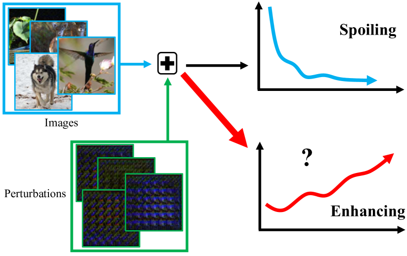
Figure 1: Bidirectional control of classification performance using small additive perturbation. Various approaches have shown that CNN based classifiers can be easily fooled. Our model aims to find the perturbation that can control the CNN classification performance in both directions: enhancement, and degradation.

These works show that it is possible to control the target performance through small external changes without modifying the values of network parameters, suggesting that it is possible to generate a perturbation to improve the performance of the model. Regarding the issue of generating adversarial perturbation, studies including privacy applications [34, 23, 33] and defenses of the adversarial perturbation [12, 25] have been proposed so far. However, to the best of our knowledge, designing a perturbation that enhances the performance of a model has not been proposed yet.

In this paper, we propose a new general framework for generating a perturbation vector that can either enhance or worsen the classification accuracy. The proposed algorithm solves two main problems. First and most importantly, our model generates a perturbation that enhances classification performance without changing the network parameters (enhancing problem). It is worth noting that this is the first attempt to show that performance-enhancing perturbations exist. Second, our algorithm generates a perturbation vector so as to lower the classification performance of the classifier (adversarial problem). For the adversarial problem, our algorithm can generate perturbations without knowing the structure of the network being used, which is difficult for existing adversarial algorithms [26, 28, 11].

To solve this problem, we propose a perturbation vector generation network (PGN) consisting of two sub-networks: generator and discriminator. The generator network generates a perturbation vector that coordinates the target performance in the desired direction, and the discriminator network distinguishes whether the generated perturbation is good or bad. Both networks are trained through minimax games inspired by generative adversarial nets (GAN) [10], and the resultant perturbation vector from the generator controls the result of the target classifier networks. However, unlike those of the variants of GAN [10, 24, 35, 4], the purpose of the proposed minimax framework is to generate additive noises that help the input data satisfy the desired goal of performance-enhancement or degradation, not generating a plausible data samples. The main contributions of the proposed work can be summarized as follows:

• We show the existence of a perturbation vector that enhances the overall classification result of a dataset.

• We propose a unified framework of PGN that can solve the performance-enhancement, and the adversarial problem.

• We show that the proposed method can generate perturbation vectors that can solve the adversarial problem without knowing the structure of the network.

The proposed method has been validated with a couple of public datasets: the STL-10 dataset [5], and subsets of the ImageNet dataset [40]. Also, widely used classifier networks such as ResNet [14], VGGnet [42], and DenseNet [16] have been tested as the target classifier.

2 Related Work

In contrast to the great success of CNN in various image recognition tasks [42, 44, 14, 43], many studies [3, 45, 28, 2, 41, 46, 7, 8, 38, 39, 11, 26, 27, 29] have indicated that CNNs are not robust and are easily fooled. Szegedy et al. [45] discovered that such classification networks are vulnerable to well-designed additive small perturbations. These perturbation vectors can be estimated either by solving an optimization problem [45, 28, 2] or by one-step gradient ascent of the network [11]. Also, studies [30, 31] have been published that show the difference between CNNs and humans in understanding an image. These works generate a perturbation vector depending both on the input image and on the network used. On the other hand, the work in  [13] generate an image-specific universal adversarial perturbation vector valid for arbitrary networks, while [26, 27, 29] find a universal adversarial perturbation vector independent of images.

The discovery of an adversarial example has attracted a great deal of attention in relation to privacy issues [34, 23, 33], and many studies have been published on the privacy and defense [12, 25, 49, 22, 6, 15] of adversarial examples. Studies have also been proposed for tasks such as transferring the adversarial example to other networks [20, 4], transforming an input image to its target class by adding a perturbation [1], and generating an adversarial perturbation vector [48] for segmentation and detection.

The main issues we deal with in this paper are different from those in the studies mentioned above. Unlike the previous works focusing on the adversarial problem and its defense, our works mainly aim to propose a network that generates a perturbation vector that can enhance the overall classification performance of the target classifier. Furthermore, in addition to the enhancing problem, the proposed network is designed so that it is also applicable to the adversarial problem with an unknown black-box target classifier.

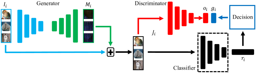
Figure 2: Framework of the proposed method. For controlling the performance of the target classifier (Black), a perturbation $M_{i}$ (Green) is generated from a base image $I_{i}$ (Blue) by the generator. The discriminator (Red) then judges if the perturbation has adjusted the classification result as desired.

3 Proposed Method

3.1 Overview

In an image classification framework, we are given a set of labeled images $T=\{(I_{i},l_{i}),i=1,...,N\}$ and classifier $r_{i}=f_{c}(I_{i})$, where $I_{i}$ and $l_{i}$ denote the image and the corresponding label, respectively, and the resultant label $r_{i}$ belongs to one of the class labels $r_{i}\in\{c_{1},...,c_{K}\}$. Given this condition, our goal is to generate an additive perturbation vector $M_{i}$ that can control the classification result of the classifier $f_{c}(\cdot)$, given an image $I_{i}$. The generated perturbation vector $M_{i}$ is added to the image $I_{i}$ as

$$J_{i}=I_{i}+\lambda M_{i},$$ (1)

and the classification result $f_{c}(J_{i})$ of the perturbed image $J_{i}$ should be controlled by the vector $M_{i}$ so as to solve the two listed problems: the enhancing problem  and the adversarial problem.

For the enhancing problem, we aim to generate a perturbation vector under the condition where the classifier network is accessible, but with fixed parameters. For the adversarial problem, our model solves the problem under the situation that the classifier network is not accessible at all (Black Box).

3.2 Perturbation Generation Network

Figure 2 describes the overall framework of the proposed PGN, which mainly consists of three networks: a generator, a discriminator and a classifier. In our problem, only the network parameters in the generator and the discriminator will be updated.

As in equation (2), the generator network $G(I_{i};W_{G})$ generates a perturbation vector $M_{i}$ with the same size as the input image $I_{i}$, where $W_{G}$ refers to the network parameters of the generator;

$$M_{i}=G(I_{i};W_{G}).$$ (2)

In our model, $G(I_{i};W_{G})$ is composed of an encoder network $v=E(I_{i};W_{enc})$ and decoder network $M_{i}=D(v;W_{dec})$, where $W_{G}=\{W_{enc},W_{dec}\}$. Using the vector $M_{i}$ and the image $I_{i}$, we get a perturbed image $J_{i}$ as in equation (1). The perturbed image $J_{i}$ then bifurcates as inputs to the classifier $f_{c}(J_{i})$ as well as the discriminator $D(J_{i})$. In our model, the discriminator $D(J_{i};W_{D})$ is designed as a network with a sigmoid output as in equation (3) to judge whether $J_{i}$ is generated according to our purpose, by using the classification result of the given target classifier $f_{c}(\cdot)$;

$$o_{i}=D(J_{i};W_{D}),~{}o_{i}\in[0,1].$$ (3)

Here, the term $W_{D}$ denotes the network parameters of the discriminator, and the term $o_{i}$ is a sigmoid scalar unit. The important thing here is to set the target variable $g_{i}$ for the output $o_{i}$ of the discriminator to fit the purpose of the problem we aim to solve. Then, the loss functions for training the generator and discriminator networks are defined using $g_{i}$ and $o_{i}$. For each of the two problems we want to solve in this work, detailed explanations will be presented in what follows. The overall algorithm will be presented with the case of the enhancing problem, and the case of adversarial problem will be addressed based on the discussion.

Enhancing Problem: In order to enhance the performance of the classifier, we first define a discriminator loss to let the network determine whether the generated perturbed image $J_{i}$ is good or bad. When the classification result of the generated image $J_{i}$ matches the ground truth $l_{i}$, we set the target $g_{i}$ as $1$ (good), and otherwise $0$ (bad) as follows:

$$g_{i}=\begin{cases}1,~{}r_{i}=l_{i},\\ 0,~{}r_{i}\neq l_{i}.\end{cases}$$ (4)

Here, $r_{i}=f_{c}(J_{i})$ and $l_{i}$ is the ground truth class label for $I_{i}$. Using the target variable $g_{i}$, the discriminator and the generator losses are defined in the sense of mean squared error as in equations (11) and (12), respectively;

$$L_{d}=\frac{1}{2}\mathbf{E}_{p_{g}}[{(D(J)-1)}^{2}]+\frac{1}{2}\mathbf{E}_{p_{\bar{g}}}[{(D(J))}^{2}],$$ (5)

$$L_{g}=\frac{1}{2}\mathbf{E}_{p_{g}}[{(D(J)-1)}^{2}]+\frac{1}{2}\mathbf{E}_{p_{\bar{g}}}[{(D(J)-1)}^{2}].$$ (6)

The distributions $p_{g}$ and $p_{\bar{g}}$ denote $p(g=1)=p(r=l)$ and $p(g=0)=p(r\neq l)$, respectively. Note that both $r$ and $g$ depends on the generated sample $M$.

In practice, the expectations in (11) and (12) are replaced with empirical means as follows:

$$L_{d}=\frac{1}{2}\sum_{i}[g_{i}{(D(J_{i})-1)}^{2}+(1-g_{i}){D(J_{i})}^{2}]$$ (7)

$$L_{g}=\frac{1}{2}\sum_{i}{(D(J_{i})-1)}^{2}.$$ (8)

These generator and discriminator losses are inspired by least-square GAN (LSGAN) [24], and we train the discriminator and generator networks to minimize each loss with respect to $W_{D}$ and $W_{G}$, respectively. However, our formulation is different from that of [24] as clearly shown in (8). The proposed scheme is designed to make every $D(J_{i})$ converge to $1$, which means that our learning scheme reaches the proposed goal of enforcing correct classification. In implementation, $\ell_{1}$ regularization loss $L_{r}=\frac{1}{N}\sum_{i}{\|M_{i}\|}_{1}$ is added to the generator loss in equation (8) to control the intensity of the perturbation, as the following:

$$L_{g^{\prime}}=L_{g}+\gamma L_{r}.$$ (9)

Qualitatively, minimizing the loss in equation (11) means that the output of the discriminator $D(J_{i})$ goes to $1$ when $g_{i}$ equals to $1$ (good), and goes to $0$ in the opposite case (bad). Similarly, minimizing $W_{G}$ of the generator implies that $M_{i}=G(I_{i})$ is trained so that the output of the discriminator $D(J_{i})$ goes to $1$ in every case, by deceiving the discriminator. We have shown the proposed minimax game using the equations (11),(12) theoretically makes $p_{g}(J_{i})$ converge to $1$. We have also proven that similar to [10], this scheme is valid when a cross-entropy loss is applied instead of least-square loss in (11) and (12). Detailed explanation and proof are provided in Appendix A.

Adversarial Problem: We can generate an adversarial perturbation vector $M_{i}$ without much changing the previously described model for the performance enhancement problem. In the case of the adversarial problem, the discriminator should count the vector $M_{i}$ as success when the classification result $f_{c}(J_{i})$ becomes different from the ground truth $l_{i}$. Therefore, in this case, the target vector $g_{i}$ is defined as in equation (10),

$$g_{i}=\begin{cases}1,~{}r_{i}\neq l_{i},\\ 0,~{}r_{i}=l_{i}.\end{cases}$$ (10)

From the experiments, the proposed minimax framework with the discriminator and the generator losses defined as in equations (7) and (8) has sufficient capacity to drop the classification performance. One thing that is worth mentioning is that the existing works solve the problem based on the assumption that the network framework is given while we can do so without knowing the network framework.

Algorithm 1 Training procedure of the proposed PGN.

1:Training data $\{I_{i},l_{i}\}$, target classifier $f_{c}(\cdot)$.

2:Trained PGN weights $W_{G}$ and $W_{D}$

3:Initialize $W_{G}$ and $W_{D}$

4:repeat

5:     $J_{i}\leftarrow I_{i}+\lambda M_{i},~{}M_{i}\leftarrow G(I_{i};W_{G})$, in eq. (1), (2).

6:     $r_{i}\leftarrow f_{c}(J_{i})$.

7:     $o_{i}\leftarrow D(J_{i};W_{D})$, in eq. (3).

8:     Get $g_{i}$ using $r_{i}$ by eq. (4) or (10)

9:     Get $L_{d}$ from $o_{i}$ and $g_{i}$, using eq. (7).

10:     Update $W_{D}$ using $L_{d}$

11:     $o_{i}\leftarrow D(J_{i};W_{D})$, in eq. (3).

12:     Get $L_{g}$ from $o_{i}$, $r_{i}$, and $l_{i}$, using eq. (9).

13:     Update $W_{G}$ using $L_{g}$.

14:until $L_{g}$ converges

(A)

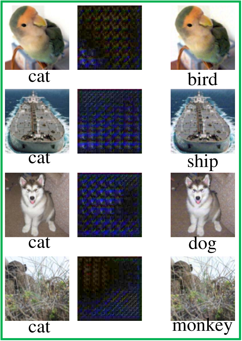
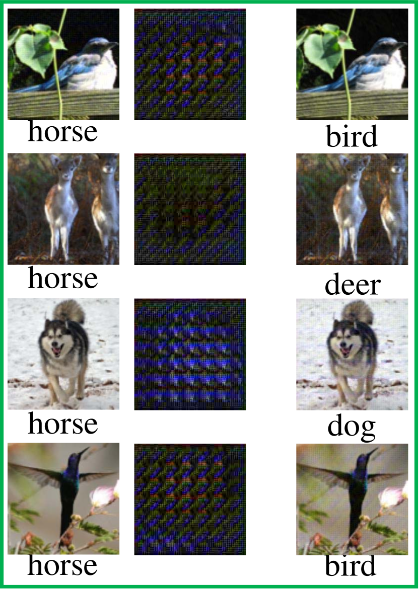
(B)

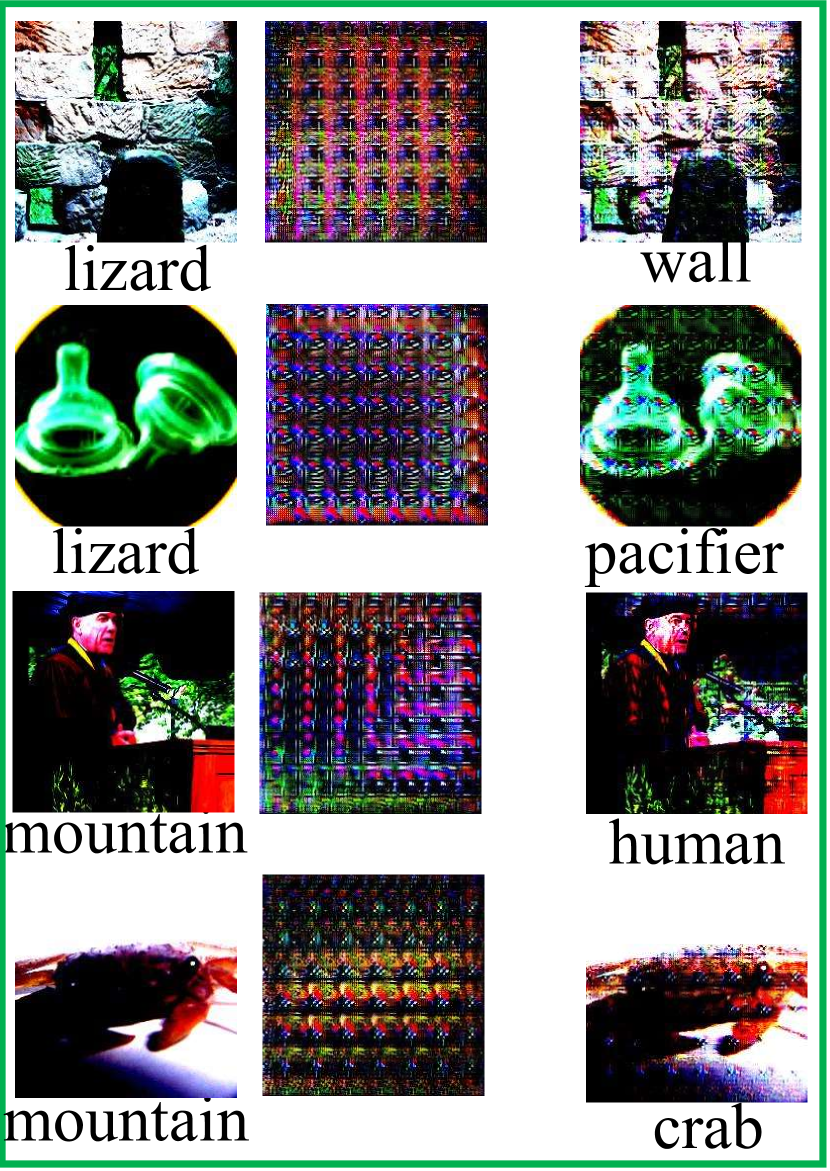
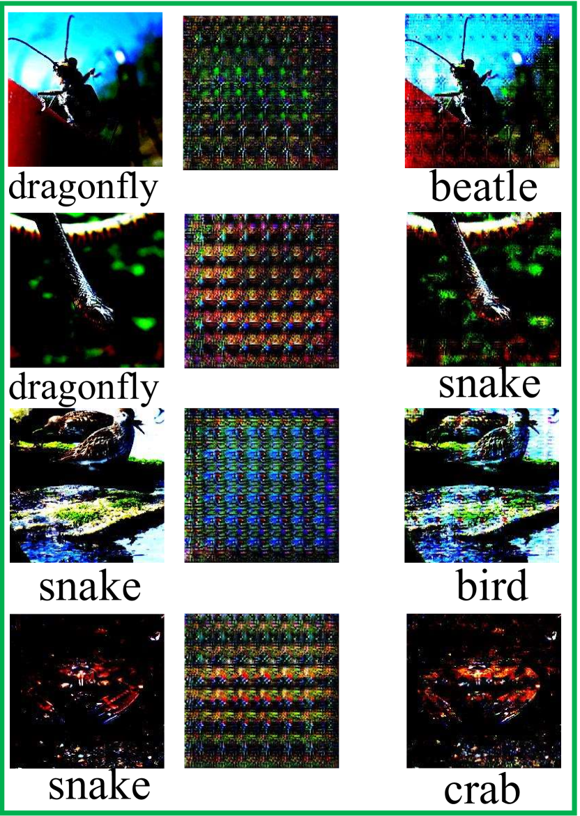
Figure 3: Examples of the triplets for the enhancing problem: original image (left), generated perturbation (mid), and perturbed image (right). The examples in (A) denote the case when we use vanilla images, and those in (B) show the results from normalized images. Intensity of the perturbation in (A) is ten times amplified for visualization. (Best viewed in color)

3.3 Training

By using the defined variables and loss terms, we can train the proposed network in a similar way to the adversarial min-max training as introduced in [10]. The pseudo-code in Algorithm 1 describes the detailed training scheme of the proposed algorithm. For each iteration, we first generate perturbation vector $M_{i}$ and check if the perturbation satisfies the desired goal in the form of target vector $g_{i}$. After setting $g_{i}$, same as usual advesarial frameworks, we train the discriminator network with given peturbation. Then, we re-calculate the output value $o_{i}$ of the discriminator using the updated discriminator and update the generator to deceive the discriminator.

In our implementation, the network parameters are updated by Adam optimizer [17]. We used fixed learning rate $lr=0.0001$ to train both the generator and the discriminator, and stopped the iteration at $20$ epoch, in practice. The additive parameter $\lambda$ is set to $1$ for the entire experiments.

3.4 Implementation Detail

The proposed algorithm is ideally independent of a classifier. However, the Nash-equilibrium [10, 24] for general adversarial framework is difficult to find, and hence an efficient design of initial condition is required. Thus, For the enhancing problem, we initialize the discriminator network with the weight parameters of target classifier. In this case, we share the classification network with the discriminator, and only a fully connected layer with sigmoid activation is additionally trained. For the adversarial problem, both cases of known and unknown classifier structure are considered. In unknown case, we apply ResNet101 network for the discriminator. For the known case, the same network as target classifier is used. In both known and unknown cases, ImageNet pre-trained parameters are used to initialize the discriminator, and the final fully connected layers are trained.

The generator network of the proposed algorithm consists of an encoder and a decoder. We applied the Imagenet pre-trained ResNet for the encoder with a layer size of 50 or 101, respectively. To define the decoder, we use four deconvolution blocks each consisting of three deconvolution layers with filter size $4\times 4$, $3\times 3$, and $3\times 3$, and one final deconvolution layer with filter size $4\times 4$ and stride $2$. For each deconvolution block, the stride of the first deconvolution layer is set to $2$, and those of the last two deconvolution layer are set to $1$. The numbers of channels for the total $13$ deconvolution layers are set to $2048,$$1024,512,512,256,256,256,128,128,128,64,64$, and $3$.

4 Experiments

Now, we validate the performance of the proposed algorithm for the two presented problems: the enhancing problem and the adversarial problem. Since this is the first attempt to solve the enhancing problem, we analyze the proposed network by varying parameters and networks. For the adversarial problem, we compared the performance of the proposed algorithm with those of two representative algorithms that utilize target classifier information, since there has not been any algorithms proposed to solve the adversarial problem without knowing the target classifiers.

4.1 Experimental Settings and Datasets

In the experiment, we examined recent classifiers such as ResNet [14] ($50,101$), VGG [42], and DenseNet ($169$) [16] as target classifiers to be controlled. For the encoder $E(\cdot)$ of the generator network, we tested two cases, each of which uses ImageNet pre-trained ResNet $101$ (Proposed-101) and ResNet $50$ (Proposed-50) as a base type of the proposed model, respectively. We also analyzed the effect of regularization loss $L_{r}$ by testing different regularization parameter $\gamma$ for both the enhancing and the adversarial problems. For the adversarial problem, the proposed algorithm is also tested with a black-box version ‘Proposed-B’ whose network structure is unknown. The adversarial performance is compared to the works of Moosavi et al. (UAP) [26] and Goodfellow et al. (EHA) [11]. In all the experiments, STL-10 dataset [5] and subsets of ImageNet dataset [40] were used. To form the subsets of ImageNet dataset, 10 and 50 classes were randomly selected, respectively. To verify the effect of image normalization, we experimented with the STL-10 dataset without normalization and performed same tests on the ImageNet subset with normalization applied. All the images are scaled to $224\times 224$ in the experiments. For main analysis, we set $\gamma=0.0001$ for the enhancing problem (Figure 3 and Table 1) and set $\gamma=3$ for the adversarial problem (Figure 5 and Table 2). Target classifiers (Vanilla) were trained with $lr=0.0005$ and $20$ iterations, which sufficient for convergence.

Table 1: Top-$1$ precision and mAP scores for performance enhancing problem: $\gamma$ = 0.0001

Dataset	Classifier	Encoder from scratch [A]			Imagenet Pre-trained encoder [B]
		Vanilla	Proposed-50	Proposed-101	Vanilla	Proposed-101
stl-10	ResNet50	61% / 0.588	78.1% / 0.760	84.9% / 0.826	92.0% / 0.883	93.6% / 0.890
	ResNet101	63% / 0.570	84.1% / 0.785	89.6% / 0.852	93.0% / 0.896	94.2% / 0.907
	VGG16	52% / 0.518	92.4% / 0.903	91.3% / 0.866	83.4% / 0.757	94.6% / 0.930
	DenseNet169	65% / 0.564	86.5% / 0.781	89.7% / 0.829	95.4 % 0.884	95.9% / 0.897
ImageNet-10	ResNet50	78% / 0.685	96.0% / 0.927	91.6% / 0.871	98.0% / 0.969	99.0% / 0.974
	ResNet101	77% / 0.666	93.6% / 0.898	90.4% / 0.871	98.0% / 0.970	98.6% / 0.972
	VGG16	71% / 0.613	95.4% / 0.886	96.2% / 0.900	94.8% / 0.936	96.0% / 0.927
	DenseNet169	77% / 0.659	97.0% / 0.936	93.4% / 0.884	98.0% / 0.970	99.0% / 0.971
ImageNet-50	ResNet50	72% / 0.649	91.5% / 0.883	91.3% / 0.886	94.4% / 0.922	95.6% / 0.928
	ResNet101	71% / 0.635	89.0% / 0.856	88.1% / 0.832	95.7% / 0.938	96.7% / 0.949
	VGG16	71% / 0.616	93.4% / 0.894	94.2% / 0.902	88.5% / 0.855	92.0% / 0.906
	DenseNet169	74% / 0.626	92.1% / 0.861	93.1% / 0.875	95.5% / 0.927	96.3% / 0.934

4.2 Enhancing Problem

Main Analysis: Figure 3 (A) shows the examples of the generated perturbation mask for the enhancing problem from STL-10 images without normalization, i.e. pixel values are in between 0 and 1. In (A), the original images are misclassified to a cat or a horse, respectively. However, if the proposed perturbation is added to the misclassified original image, we can see that the target classifier correctly classifies the image. Figure 3 (B) presents similar results from the normalized images of ImageNet dataset, i.e. pixel values are normalized to have zero mean and unit variance. In the figure, we can see that originally misclassified examples are correctly classified by adding the corresponding perturbations generated. These corrections are remarkable in that the perturbations are small enough that they do not compromise the main characteristics of the original image, and do not resemble the shape of the correct target classes.

(A)

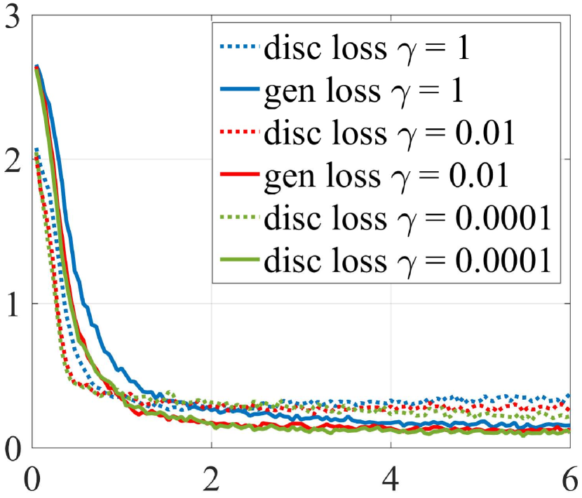
(B)

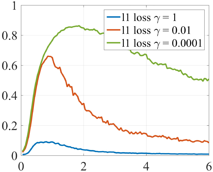
(C)

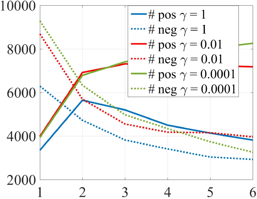
(D)

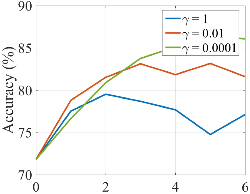
Figure 4: Graphs describing the convergence and performance enhancement of the proposed algorithm with different $\gamma$: (A) discriminator loss and generator loss, (B) $\ell$1-loss, (C) positive and negative samples in training set, (D) Accuracy. Horizontal axis denotes epoch. The experiments were performed with the ResNet101 classifier on ImageNet50 using the ‘Proposed-50’.

Table 1 presents the quantitative results showing the enhanced performance of the proposed algorithm. Experiments were conducted on two cases of classifier: (A) classifiers trained from scratch, (B) classifiers trained from ImageNet pre-trained net. For both cases, we set the target classifiers to evaluation the mode which excludes the randomness of the classifiers, such as that caused by batch normalization or drop-out, which are usual settings for deep learning testing. In Table 1(A), two proposed versions, ‘Proposed-50’ and ‘Proposed-101’, were examined to discover whether the proposed algorithm is affected by the structure of the encoder. The result shows that the proposed algorithm can enhance the classification performance of the listed target classifiers for both versions in every dataset, and the performance difference is not significant for the two versions. It is also worth noting that in many cases, the classification performance enhancement by the proposed perturbation is comparable to the results of the fine-tuned network initialized with the ImageNet pre-trained parameters. In particular, the VGG network achieved the highest classification performance enhancement by the proposed method. This is meaningful in that it shows that our perturbation can compensate for the insufficient information of the classifier.

In Table 1(B), the performance-enhancing results from ‘Proposed-101’ for ImageNet pre-trained classifiers are presented. In this case, the classification performance of the vanilla classifiers is obviously higher than that of the scratch-trained version, and hence it is more difficult to enhance the performance. Nevertheless, our algorithm has succeeded in improving performance for all the listed cases. In particular, we confirmed that the VGG classifier had more performance improvement than the other recent classifiers such as ResNet and DenseNet, and the performance gaps between VGG and these recent classifiers were decreased by adding the perturbation. This is meaningful in that it shows the possibility that a relatively simple network like VGG can get better performance.

(A)

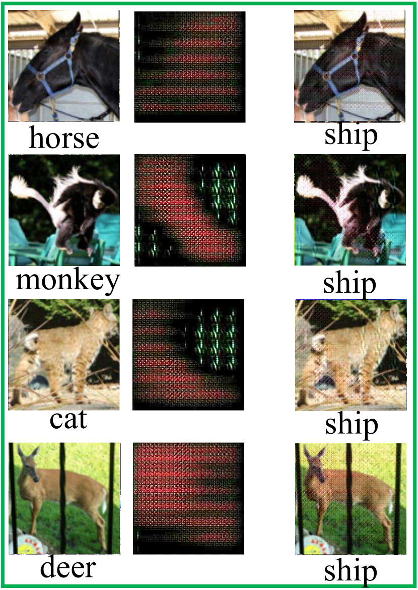
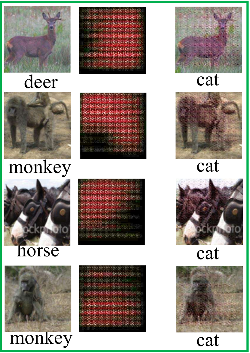
(B)

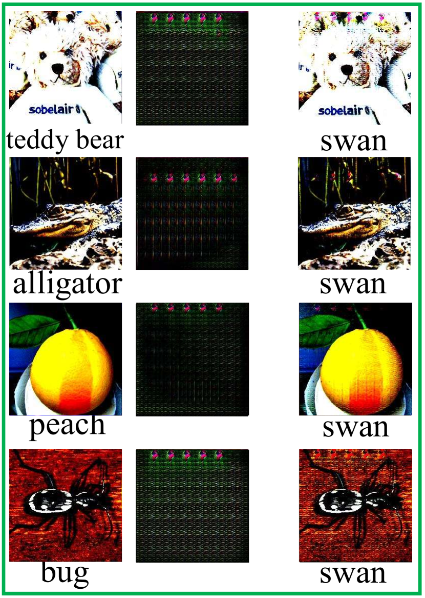
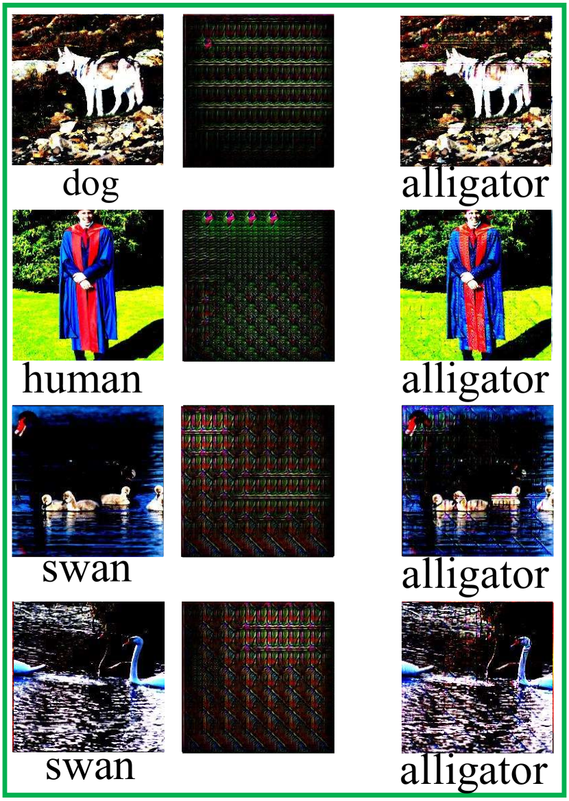
Figure 5: Examples of the triplets for the adversarial problem: original image (left), generated perturbation (mid), and perturbed image (right). The examples in (A) denote the case when we use vanilla images, and those in (B) show the results from normalized images. Intensity of the perturbation in (A) is ten times amplified for visualization. (Best viewed in color)

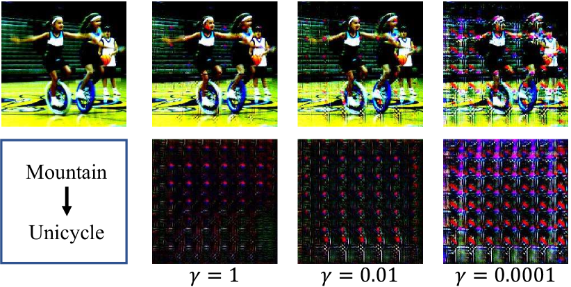
Figure 6: Example perturbed images from the enhancing problem with different $\gamma=1,0.01,$ and $0.0001$.

Convergence and $\bm{\ell 1}$-Regularization: The graphs in Figure 4 describe the change of losses as the epoch progresses. The generator loss $L_{g}$, the discriminator loss $L_{d}$, and the $\ell 1$-loss $L_{r}$ are plotted with different $\gamma$’s in equation (9). As shown in the graph (A), both $L_{g}$ and $L_{d}$ converge for every setting of $\gamma$, as desired. Also, $L_{r}$ showed a similar convergence tendency for different $\gamma$, as in the graph (B). However, as $\gamma$ decreases, the time $L_{r}$ start to decrease delayed, and the maximum value of $L_{r}$ increased. From the graphs (C) and (D), We can see that these changes of $L_{r}$ have a direct impact on the enhancing performance. The graph (C) describes the number of positive (false to correct) and negative (correct to false) samples in training set for every epoch. As seen in the graph, The number of positive samples were increased and that of negative samples were decreased until the $\ell 1$ intensity of the perturbation fell below a certain level. We can also see through graph (D) that the accuracy did not rise from the point where the increase of the gap between positive and negative samples is slowed down. In summary, the amount of possible performance enhancement and $\ell 1$-regularization is a trade-off relationship, and the amount can be adjusted depending on how much perturbation is allowed.

The qualitative result of perturbed images for different $\gamma$ is presented in Figure 6. In the example, we can see that the image changes more to correct the classification result as $\gamma$ becomes smaller. We confirmed from graph (C) that the performance improvement was about $10\%$ even when $\gamma=1$, and the change in the image would be very small in this case. In fact, it may be wise to remove the $\ell 1$ regularization term if performance gains are only concerned. The analysis is presented in Appendix A.

4.3 Adversarial Problem

Main Analysis: The example adversarial results from the proposed algorithm are presented in Figure 5. The black box version ‘Proposed-B’ was used for the results in the figure, and we can see that the classification results can be changed by adding small perturbations for both normalized and original images. It is noteworthy that the appearances of the perturbations produced by the normalized images and those of the non-normalized images are largely different.

Table 2 shows the performance drop by the adversarial perturbation. In most cases, the proposed algorithm achieved better adversarial performances than the conventional algorithms [26, 11] in both cases of known and unknown classifier network. We also confirmed that the proposed algorithm successfully degrades performance, regardless whether the image is normalized. What is noteworthy is that even if there is no information in the target classification network, the adversarial performances were not largely degraded compared to the case of known network information. This is significant in that the proposed algorithm enables more realistic applications than existing algorithms that require a network structure, because the structure of the classifier is usually concealed.

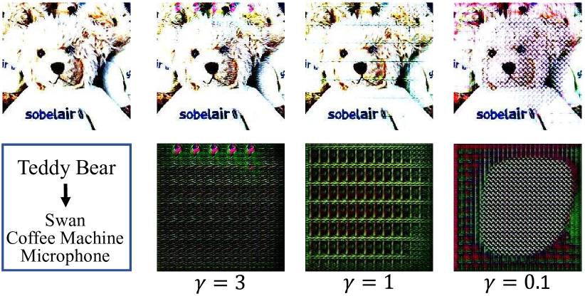
Figure 7: Example perturbed images from the adversarial problem with different $\gamma=3,1,$ and $0.1$.

Table 2: Quantitative result for adversarial problem

Quantitative result for adversarial problem: $\gamma$ = 3
Dataset	Classifier	Vanilla	Proposed-50	Proposed-101	proposed-B	UAP [26]	EHA [11]
stl-10	ResNet50	92.0% / 0.883	5.00% / 0.071	5.15% / 0.052	6.92% / 0.073	24.0% / 0.176	20.4% / 0.141
	ResNet101	93.0% / 0.896	6.60% / 0.081	5.32% / 0.056	9.30% / 0.094	22.3% / 0.175	31.2% / 0.200
	VGG16	83.4% / 0.757	7.00% / 0.043	1.00% / 0.028	7.49% / 0.090	9.9% / 0.099	77.7% / 0.589
	DenseNet169	95.4 % 0.884	14.0% / 0.136	9.21% / 0.104	2.80% / 0.038	22.9% / 0.169	19.4% / 0.145
ImageNet-10	ResNet50	98.0% / 0.969	6.10% / 0.071	9.80% / 0.110	12.4% / 0.137	53.8% / 0.319	9.60% / 0.093
	ResNet101	98.0% / 0.970	6.00 % / 0.078	7.00% / 0.086	7.80% / 0.086	31.2% / 0.212	16.6% / 0.137
	VGG16	94.8% / 0.936	4.00% / 0.064	1.00% / 0.032	5.40% / 0.049	11.0% / 0.115	73.4% / 0.311
	DenseNet169	98.0% / 0.970	5.00% / 0.053	5.80% / 0.063	3.00% / 0.039	10.0% / 0.113	14.8% / 0.146
ImageNet-50	ResNet50	94.4% / 0.922	3.72% / 0.043	5.44% / 0.052	10.8% / 0.101	25.9% / 0.162	14.2% / 0.069
	ResNet101	95.7% / 0.938	12.0% / 0.110	10.7% / 0.092	11.6% / 0.101	14.4% /0.074	19.0% / 0.088
	VGG16	88.5% / 0.855	2.00% / 0.029	2.00% / 0.022	3.20% / 0.027	2.23% / 0.021	56.4% / 0.126
	DenseNet169	95.5% / 0.927	7.04% / 0.062	8.20% / 0.074	6.56% / 0.063	39.7% / 0.272	10.8% / 0.070

(A)

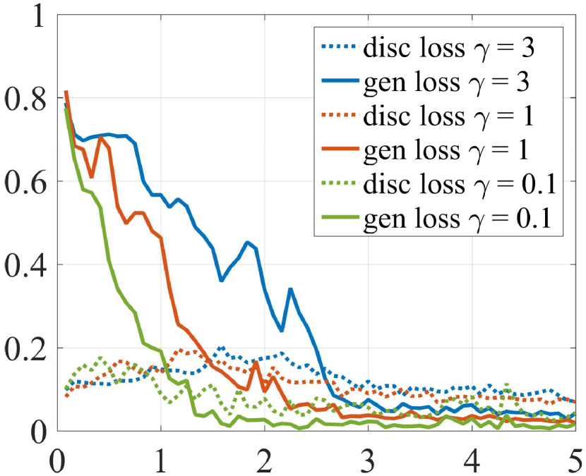
(B)

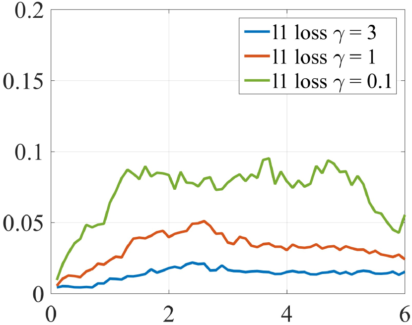
(C)

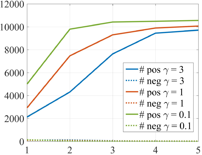
(D)

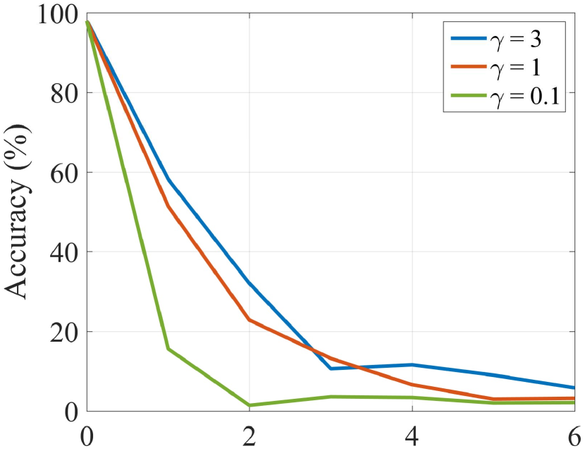
Figure 8: Graphs describing the convergence and degradation performance of the proposed algorithm for different $\gamma$: (A) discriminator loss and generator loss, (B) $\ell$1-loss, (C) positive and negative samples in training set, (D) Accuracy. Horizontal axis denotes epoch. The experiments were performed on DenseNet169 and ImageNet10 using the ‘Proposed-B’ version.

Convergence and $\bm{\ell 1}$-Regularization: Unlike with the enhancing problem, we can not expect the proposed adversarial structure to suppress the intensity of the perturbation. In the case of the enhancing problem, too much perturbation may be disadvantageous because correct image classification results should be preserved. In fact, $\ell 1$ intensity of the perturbation does not increase more than a certain level, even if there is no $\ell 1$-regularization term in the enhancing problem case. (See Appendix B for more explanation). Conversely, in the case of the adversarial problem, it can be predicted that a larger perturbation may more easily ruin the classification result. Therefore, we can conjecture that the role of $\ell 1$-regularization is very important for controlling the intensity of the perturbation in the adversarial problem.

The graphs in Figure 8 describe the changes of the loss terms in the proposed framework in the form shown in Figure 4. The one main difference to the enhancing problem is that the discriminator loss $L_{d}$ converges much faster than the enhancing problem case, as seen in graph (A). This is because, in the adversarial problem case, much more positive samples (correct to false, in this case) compared to negative samples (false to correct) can be obtained from the beginning than the enhancing problem case as shown in graph (C). This is natural in that the number of correctly classified samples in the training set is much larger than the false sample. Also, as the gamma decreases, we can see that the generator loss $L_{g}$ fluctuates drastically, which means that the $\ell 1$-loss $L_{r}$ and $L_{g}$ are in a competitive relationship. The other notable difference to the enhancing problem is that the tendency of $L_{r}$ decrease is not clear compared to the enhancing problem case. Rather, we can see that $L_{r}$ converges on different values according to the value of $\gamma$, as in graph (B). From the graph (D), we can see that the classification accuracy falls more fast when $L_{r}$ is kept at larger value, as we expected.

Figure 7 shows the amount of perturbation for different value of $\gamma$. We can see that the intensity of the perturbation get larger when $\gamma$ increases, and the deformation of the image is increased accordingly. Therefore, we performed the adversarial task for $\gamma=3$, and we obtained satisfactory performance without compromising the quality of the perturbed image significantly.

5 Conclusion

In this paper, we have proposed a novel adversarial framework for generating an additive perturbation vector that can control the performance of the classifier either in positive or negative directions without changing the network parameters of the classifier. Through the qualitative and quantitative analysis, we have confirmed that the proposed algorithm can enhance classification performance significantly by just adding a small perturbation, marking the first attempt in this field. Furthermore, we have confirmed that the proposed method can be directly applied to generate an adversarial perturbation vector that degrades classification performance, even when the framework of the target classifier is concealed, which is another first attempt. These results show that the parameters of the existing CNNs are not ideally estimated, we have made the meaningful progress toward influencing the network’s outcome in desired direction from outside.

Appendix A Convergence

In this section, we prove that our model has a global optima at $p_{g}(J)=1$, and converges to the global optima, theoretically. Also, we show that the same conditions hold when we replace the equations (11, 12) in the paper with the cross-entropy loss, which means that the discriminator is defined as a binary logistic regressor.

A.1 Proposed Case (Least Squared Problem)

In this case, we update the generator and the discriminator using the following equations:

$$L_{d}(D,G)= \frac{1}{2}\mathbf{E}_{p_{g}}[{(D(J)-1)}^{2}]+\frac{1}{2}\mathbf{E}_{p_{\bar{g}}}[{(D(J))}^{2}],$$ (11)

$$L_{g}(D,G)= \frac{1}{2}\mathbf{E}_{p_{g}}[{(D(J)-1)}^{2}]+\frac{1}{2}\mathbf{E}_{p_{\bar{g}}}[{(D(J)-1)}^{2}].$$ (12)

where the distributions $p_{g}$ and $p_{\bar{g}}$ denote $p(g=1)=p(r=l)$ and $p(g=0)=p(r\neq l)$, respectively. Note that both $r$ and $g$ depend on the generated sample $J$. Since $p_{g}$ is a function of $J$ and hence the function of $g$, we can write $L_{d}(D,G)$ and $L_{g}(D,G)$ as $L_{d}(D,p_{g}(J)),L_{g}(D,p_{g}(J))$, respectively. Therefore, our objective functions become

$$\min_{D} L_{d}(D,p_{g}(J)),$$ (13)

$$\min_{p_{g}(J)} L_{g}(D,p_{g}(J)).$$ (14)

Proposition 1.

For fixed $G$, an optimal discriminator is

$$D^{*}_{G}(J)=p_{g}(J).$$ (15)

Proof.

The training criterion for the discriminator $D$ given $G$ (in this case, $p_{g}(J)$) is conducted by minimizing the quantity $L_{d}(D,G)$

$$\begin{split}L_{d}(D,p_{g}(J))&=\int{p_{g}(J)(D(J)-1)^{2}+p_{\bar{g}}(J)(D(J))^{2}}dJ\\ &=\int{p_{g}(J)(D(J)-1)^{2}+(1-p_{g}(J))(D(J))^{2}}dJ\\ &=\int{(D(J))^{2}-2p_{g}(J)D(J)+p_{g}(J)}dJ.\end{split}$$ (16)

$\Rightarrow$: The term $L_{d}(D,p_{g}(J))$ has a local extremum at the point $D^{*}_{G}(J)$, where

$$\begin{split}\nabla_{D}L_{d}(D^{*}_{G},p_{g}(J))&=\int{2D^{*}_{G}(J)-2p_{g}(J)}dJ\\ &=0.\end{split}$$ (17)

Therefore, a sufficient condition for an optimal $D^{*}_{G}(J)$ becomes

$$D^{*}_{G}(J)=p_{g}(J).$$ (18)

$\Leftarrow$: From equation (19), The discriminator loss function is converted as

$$\begin{split}L_{d}(D,p_{g}(J))&=\int{p_{g}(J)(D(J)-1)^{2}+p_{\bar{g}}(J)(D(J))^{2}}dJ\\ &=\int{(D(J))^{2}-2p_{g}(J)D(J)+p_{g}(J)}dJ.\\ &=\int{[D(J)-p_{g}(J)]^{2}}dJ+1-\int{(p_{g}(J))^{2}}dJ~{}~{}~{}~{}\because\int{p_{g}(J)}dJ=1,\\ &=\int{[D(J)-p_{g}(J)]^{2}}dJ+C.\end{split}$$ (19)

Therefore, the term $L_{d}(D,p_{g}(J))$ achieves its minimum over $D$ necessarily at the point $D^{*}_{G}(J)$ where

$$D^{*}_{G}(J)=p_{g}(J).$$ (20)

∎

Proposition 2.

For the optimal $D^{*}_{G}(J)=p_{g}(J)$, the optimal generator is achieved at

$$p^{*}_{g}(J)=1.$$ (21)

Proof.

The training criterion for the generator $G$, hence $p^{*}_{g}(J)$ is obtained by minimizing the quantity $L_{g}(D^{*}_{G},p_{g}(J))$

$$\begin{split}L_{g}(D^{*}_{G},p_{g}(J))&=\int{p_{g}(J)(D^{*}_{G}(J)-1)^{2}+p_{\bar{g}}(J)(D^{*}_{G}(J)-1)^{2}}dJ\\ &=\int{p_{g}(J)(D^{*}_{G}(J)-1)^{2}+(1-p_{g}(J))(D^{*}_{G}(J)-1)^{2}}dJ\\ &=\int{(D^{*}_{G}(J)-1)^{2}}dJ\\ &=\int{(p_{g}(J)-1)^{2}}dJ\quad\because D^{*}_{G}(J)=p_{g}(J).\end{split}$$ (22)

The term $L_{g}(D^{*}_{G},p_{g}(J))$ is monotonically decreasing function in $p_{g}(J)\in[0,1]$, as

$$\begin{split}\nabla_{p_{g}}L_{g}(D^{*}_{G},p_{g}(J))&=\int{2(p_{g}(J)-1)}dJ\\ &\leq 0\quad\because 0\leq p_{g}(J)\leq 1,\forall J.\end{split}$$ (23)

Here, we wrote $\nabla_{p_{g}(J)}$ as $\nabla_{p_{g}}$ for simplicity. Therefore, the optimal $p^{*}_{g}(J)$ that minimizes $L_{g}(D_{G}^{*},p_{g}(J))$ becomes

$$p^{*}_{g}(J)=1.$$ (24)

∎

Theorem 1.

If G and D have enough capacity, and at each iterative step minimizing the equations (11) and (12), $D$ is allowed to reach the optimal given $G$, then the optimal distribution $p^{*}_{g}(J)$ converges to $1$.

Proof.

According to the proposition 2, the supremum of $U(p_{g})=\sup_{D}L_{g}(D,p_{g}(J))$ is convex. The subdifferential of $U(p_{g})$ includes the derivative of the function $L_{g}(D,p_{g}(J))$ at the point $D_{G}^{*}$ where the maximum of $L_{g}$ is attained. Applying a subgradient method to $U(p_{g})$ is equivalent to conducting the gradient descent update of $p_{g}(J)$ for the function $L_{g}(D_{G}^{*},\cdot)$. Therefore, $p_{g}(J)$ converges to the global minimum $1$ with small iterative update of $p_{g}$, concluding the proof. ∎

In practice, the generator function has limited capacity to satisfy the desired conditions, and training dataset also has limited representativeness for the test dataset. However, careful designing of the generator function with multi-layered perceptron and employing sufficient amount of training dataset, our model can achieve reasonable performance in spite of the mentioned difficulties.

A.2 Logistic Regression Case

In logistic regression case, the generator and discriminator loss are defined as follows:

$$L_{d}(D,G)= \frac{1}{2}\mathbf{E}_{p_{g}}[{-\log(D(J))}]+\frac{1}{2}\mathbf{E}_{p_{\bar{g}}}[-\log(1-D(J))],$$ (25)

$$L_{g}(D,G)= \frac{1}{2}\mathbf{E}_{p_{g}}[{-\log(D(J))}]+\frac{1}{2}\mathbf{E}_{p_{\bar{g}}}[-\log(D(J))].$$ (26)

As similar process to section A.1, we use the same objective functions in equation (13) and  (14).

Proposition 3.

For fixed $G$, the optimal discriminator is

$$D^{*}_{G}(J)=p_{g}(J).$$ (27)

Proof.

The training criterion for the discriminator $D$ given $G$ (in this case, $p_{g}(J)$) is conducted by minimizing the quantity $L_{d}(D,G)$

$$\begin{split}L_{d}(D,p_{g}(J))&=\int{p_{g}(J)\log(D(J))+p_{\bar{g}}(J)\log(1-D(J))}dJ\\ &=\int{p_{g}(J)\log(D(J))+(1-p_{g}(J))\log(1-D(J))}dJ.\end{split}$$ (28)

For all $(a,b)\in{\mathbb{R}^{2}}$, the function $x\rightarrow a\log(x)+b\log(1-x)$, $x\in[0,1]$, gets its maximum value at $x^{*}=a/(a+b)$ (see [10] for detailed explanation). Using this property, the optimal point $D^{*}_{G}(J)$ becomes

$$\begin{split}D^{*}_{G}(J)&=\frac{p_{g}(J)}{p_{g}(J)+(1-p_{g}(J))}\\ &=p_{g}(J).\end{split}$$ (29)

∎

Proposition 4.

For optimal $D^{*}_{G}(J)$, the optimal generator is achieved at

$$p^{*}_{g}(J)=1.$$ (30)

Proof.

The training criterion for the generator $G$, hence $p^{*}_{g}(J)$ is obtained by minimizing the quantity $L_{g}(D^{*}_{G},p_{g}(J))$

$$\begin{split}L_{g}(D^{*}_{G},p_{g}(J))&=-\int{p_{g}(J)\log(D^{*}_{G}(J))+p_{\bar{g}}(J)\log(D^{*}_{G}(J))}dJ\\ &=-\int{p_{g}(J)\log(D^{*}_{G}(J))+(1-p_{g}(J))\log(D^{*}_{G}(J))}dJ\\ &=-\int{\log(D^{*}_{G}(J))}dJ\\ &=-\int{\log(p_{g}(J))}dJ.\quad\because D^{*}_{G}(J)=p_{g}(J).\end{split}$$ (31)

$\Rightarrow$: derivative of $L_{g}(D^{*}_{G},p_{g}(J))$ over $p_{g}$ becomes

$$\begin{split}\nabla_{p_{g}}L_{g}(D^{*}_{G},p_{g}(J))&=-\nabla_{p_{g}}\int{\log(p_{g}(J))}dJ\\ &=-\nabla_{p_{g}}\int{\log(p_{g}(J))(\nabla_{J}p_{g}(J))^{-1}}dp_{g}\\ &=-\log(p_{g}(J))(\nabla_{J}p_{g}(J))^{-1}.\\ \end{split}$$ (32)

We wrote $\nabla_{p_{g}(J)}$ as $\nabla_{p_{g}}$, and $d{p_{g}(J)}$ as $d{p_{g}}$ for simplicity. By (LABEL:eq:derivatives), $L_{g}(D_{G}^{*},\cdot)$ has a local extremum point at $p_{g}^{*}(J)=1$, and the corresponding value $L_{g}(D^{*}_{G},p_{g}(J))=0$ at that point, which is the global minimum value.

$\Leftarrow$: Assume that $p_{g}(J)=1$ for $\forall J$. In this case, $L_{g}(D^{*}_{G},p_{g}(J))=0$ and it is the global minimum of the quantity $L_{g}(D^{*}_{G},p_{g}(J))$.

Therefore, the optimal $p^{*}_{g}(J)$ becomes

$$p^{*}_{g}(J)=1.$$ (33)

∎

Theorem 2.

If G and D have enough capacity, and at each iterative step minimizing the equations (25)(26), $D$ is allowed to reach the optimal given $G$, then the optimal distribution $p^{*}_{g}(J)$ converges to $1$.

Proof.

We follow the same steps of the proof for Theorem 1. In this case also, the supremum of $U(p_{g})=\sup_{D}L_{g}(D,p_{g}(J))$ is convex except the point $p_{g}(J)=0$, as in proposition 4 (negative log function). Therefore, $p_{g}(J)$ converges to the global minimum $1$ with small iterative update of $p_{g}$, concluding the proof. ∎

Appendix B Further Experiments

Table 3: Top-$1$ precision and mAP scores for performance enhancing and adversarial problem for Imagenet50 Dataset:
$\gamma$ = 0.0001 for the enhancing problem, $\gamma$ = 3 for the adversarial problem.

Classifier	Enhancing problem			Adversarial problem
	Vanilla (1)	Proposed-ls	Proposed-lr	vanilla (2)	proposed-m (B)	Proposed-l (B)
ResNet50	72% / 0.649	91.5% / 0.883	88.6% / 0.875	94.4% / 0.922	10.8% / 0.101	16.3% / 0.156
ResNet101	71% / 0.635	89.0% / 0.856	88.4% / 0.854	95.7% / 0.938	11.6% / 0.101	22.2% / 0.206
VGG16	71% / 0.616	93.4% / 0.894	92.6% / 0.891	88.5% / 0.855	3.20% / 0.027	8.20% / 0.078
DenseNet169	74% / 0.626	92.1% / 0.861	94.2% / 0.919	95.5% / 0.927	6.56% / 0.063	18.4% / 0.160

(A)

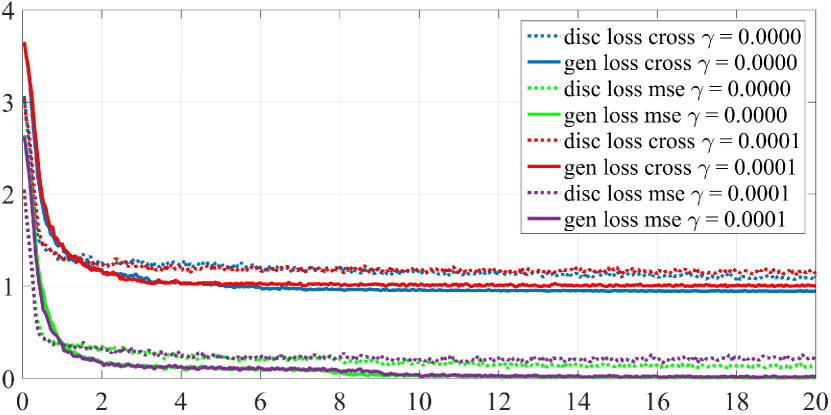
(B)

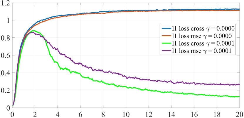
(C)

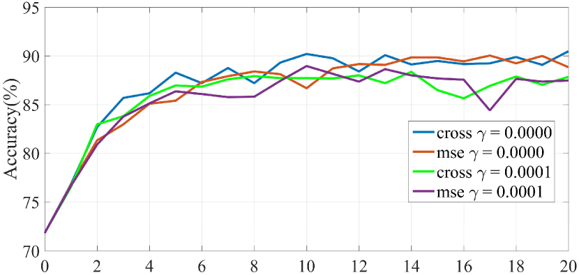
Figure 9: Graphs describing the convergence and classification performance enhancement of the proposed algorithm with different $\gamma$: (A) discriminator loss and generator loss, (B) $\ell$1-loss, (C) Accuracy. Horizontal axis denotes epoch. The experiments were performed with the ResNet101 classifier on ImageNet50 using the ‘Proposed-50’.

(A)

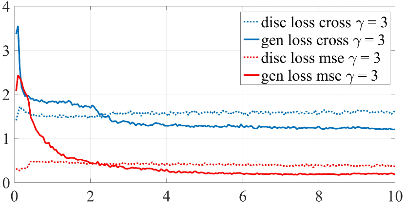
(B)

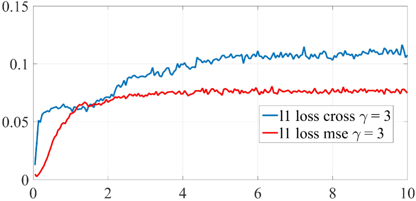
(C)

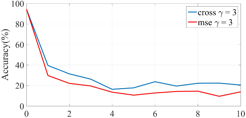
Figure 10: Graphs describing the convergence and classification performance degradation of the proposed algorithm with different $\gamma$: (A) discriminator loss and generator loss, (B) $\ell$1-loss, (C) Accuracy. Horizontal axis denotes epoch. The experiments were performed with the ResNet50 classifier on ImageNet50 using the ‘Proposed-B’.

Table 3 shows the performance enhancement and degradation of the classifiers by proposed algorithm each applying the two different loss functions: least square loss (proposed-ls), and cross-entropy loss(proposed-lr). The experiment was tested with Imagnet50, the largest dataset in the paper. For the enhancement case, we confirmed that the ‘proposed-lr’ obtained comparable results to the ‘proposed-ls’. In the degradation case, the ‘proposed-lr’ also dropped the classification performance significantly, but the decrease was smaller than that of ‘proposed-ls’ case.

In graphs in Figure 9, changes of the losses and classification accuracy over epoch for the enhancement problem are presented. As seen in the graph (A), we have confirmed that both generator and discriminator losses are converged for both ‘proposed-ls’ and ‘proposed-lr’ cases. We note that the negative log losses in ‘proposed-lr’ do not converge to zero. Interesting thing is that $\ell 1$-loss has lower value in ‘proposed-lr’ than ‘proposed-ls’. Since the performance difference between ‘proposed-lr’ and ‘proposed-ls’ is not that significant, as in graph (C), we can conclude that we can enhance the classification performance with smaller perturbation when using the cross-entropy loss than the least square loss. The graphs also show the changes of the losses in the case $\ell 1$-regularization term was detached. In this case, the $\ell 1$-intensity of the perturbation was converged to a specific value (about 1.1 as in graph (B)), as mentioned in the paper. We also confirmed from graphs (C) and (D) that excluding the $\ell 1$-regularization improved the enhancement performance, but the increase was insignificant.

Graphs in Figure 10 show the same changes presented in Figure 12 for the adversarial problem. From the graph (A), we have confirmed that the generator loss and the discriminator loss both converge for both ‘proposed-ls’ and ‘proposed-lr’. Different from the performance enhancement problem, the discriminator loss converged very fast, which is also reported in the paper. What is noteworthy is that ‘proposed-ls’ achieved better degradation performance than ‘proposed-lr’ with small $\ell 1$ intensity of the perturbation (see graphs (B) and (C)). In the adversarial problem case, it seems that applying least square loss can be more efficient choice than applying cross-entropy loss.

(A)

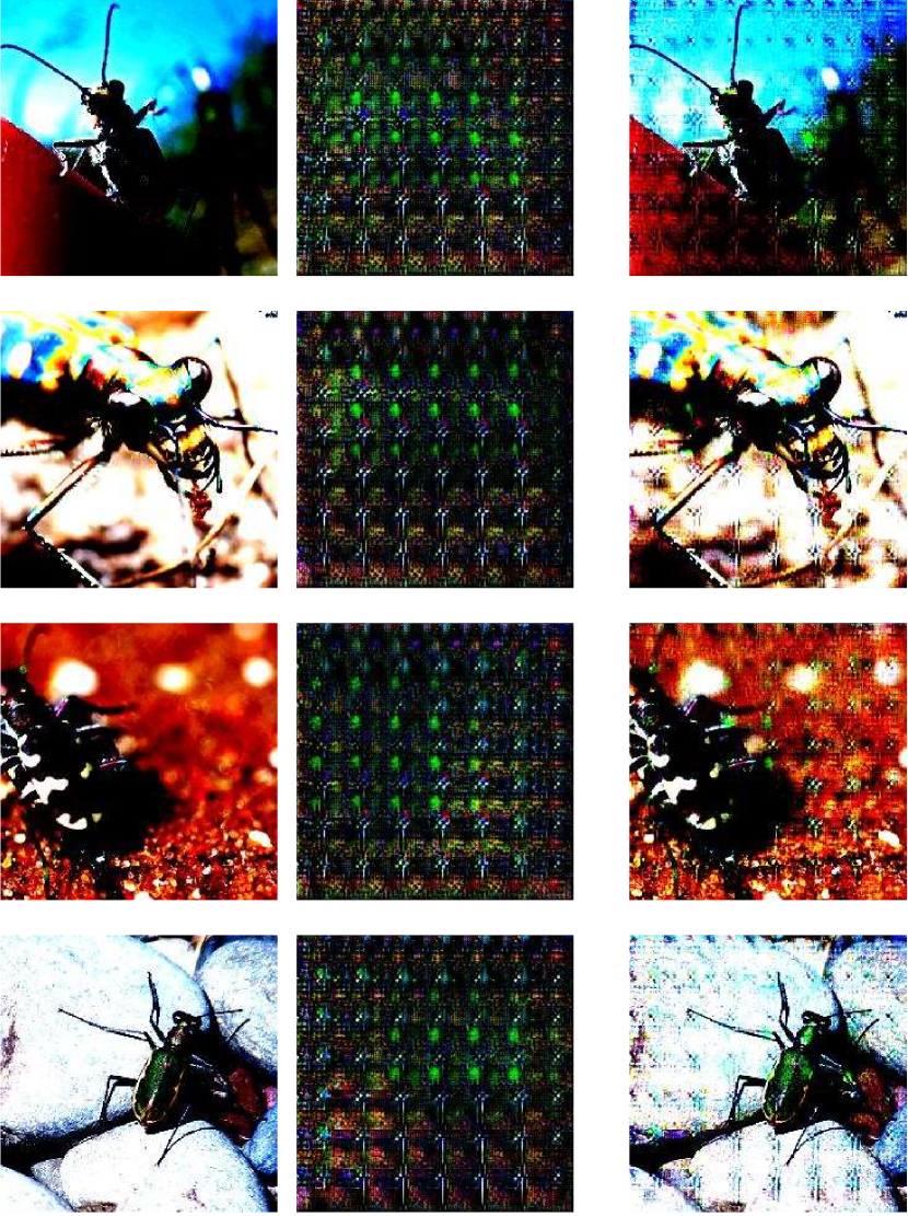
(B)

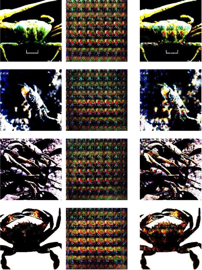
(C)

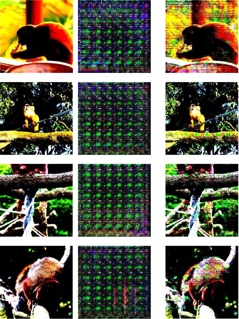
(D)

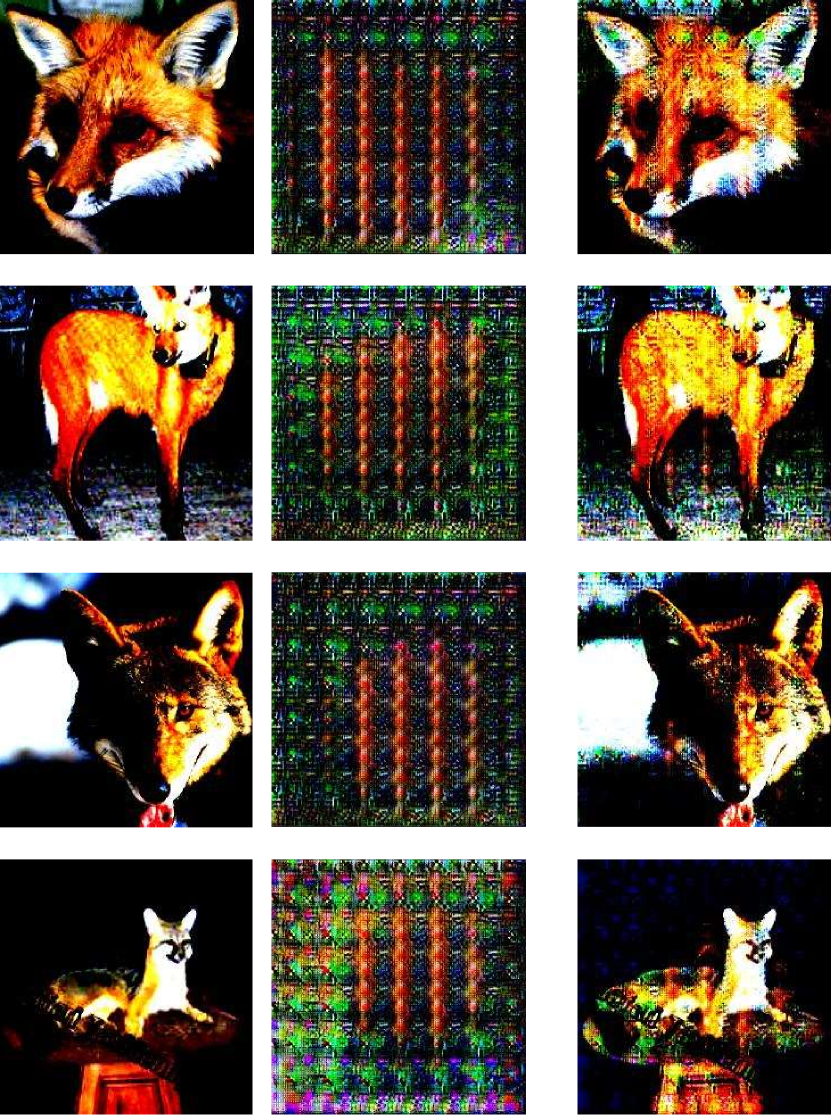
Figure 11: Examples of generated perturbation from normalized images in diverse image classes for performance enhancement problem. (A) bug, (B) crab, (C) monkey, and (D) fox.

(A)

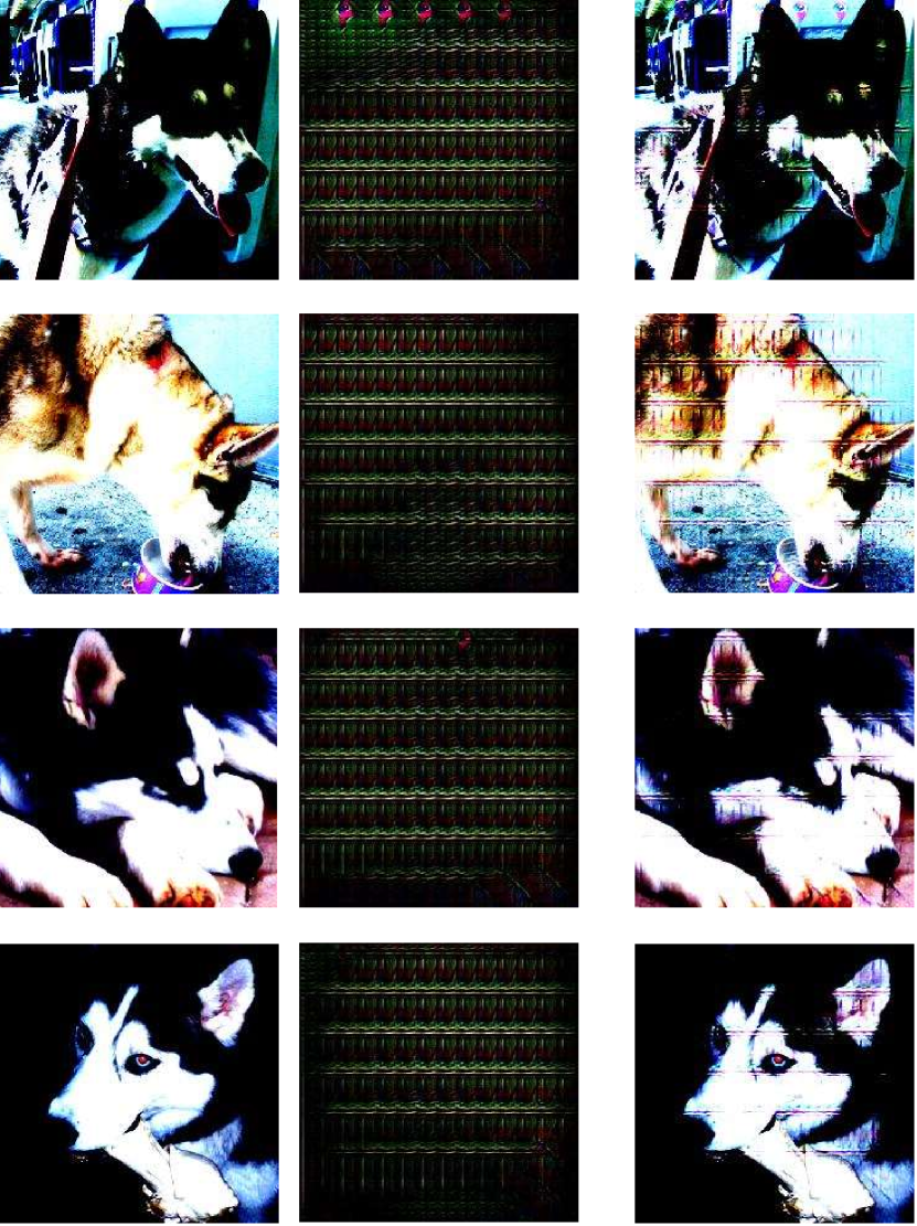
(B)

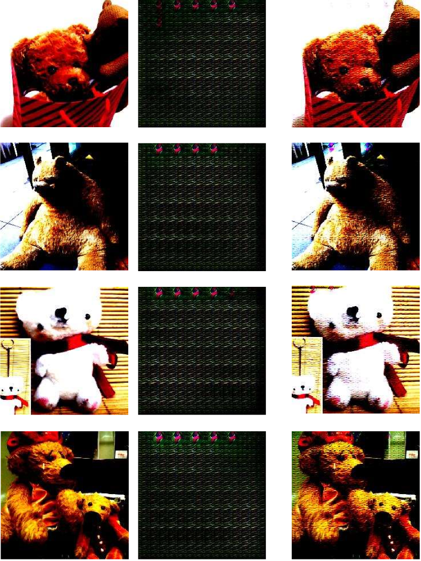
(C)

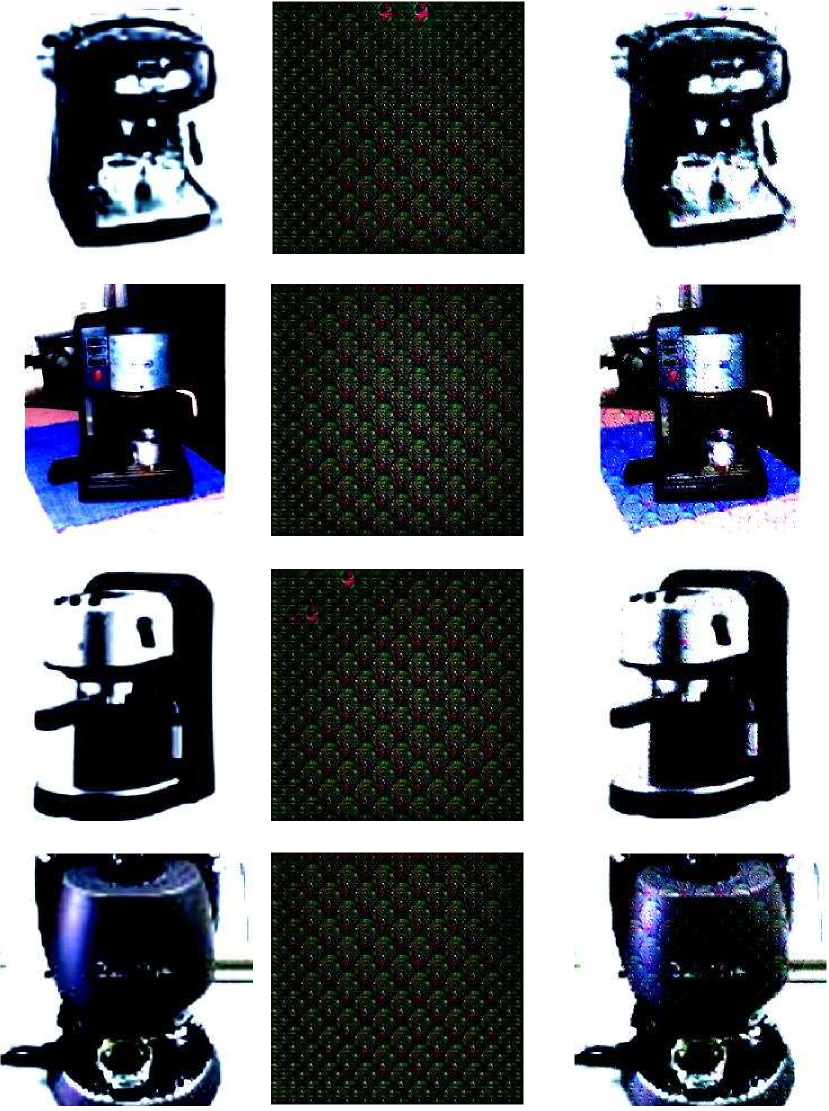
(D)

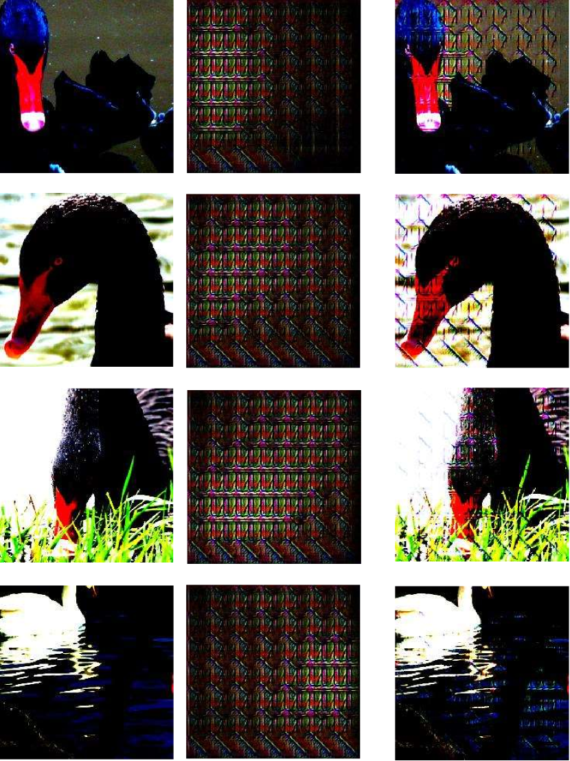
Figure 12: Examples of generated perturbation from normalized images in diverse image classes for performance degradation problem. (A) dog, (B) teddy bear, (C) coffee machine, and (D) swan.

(A)

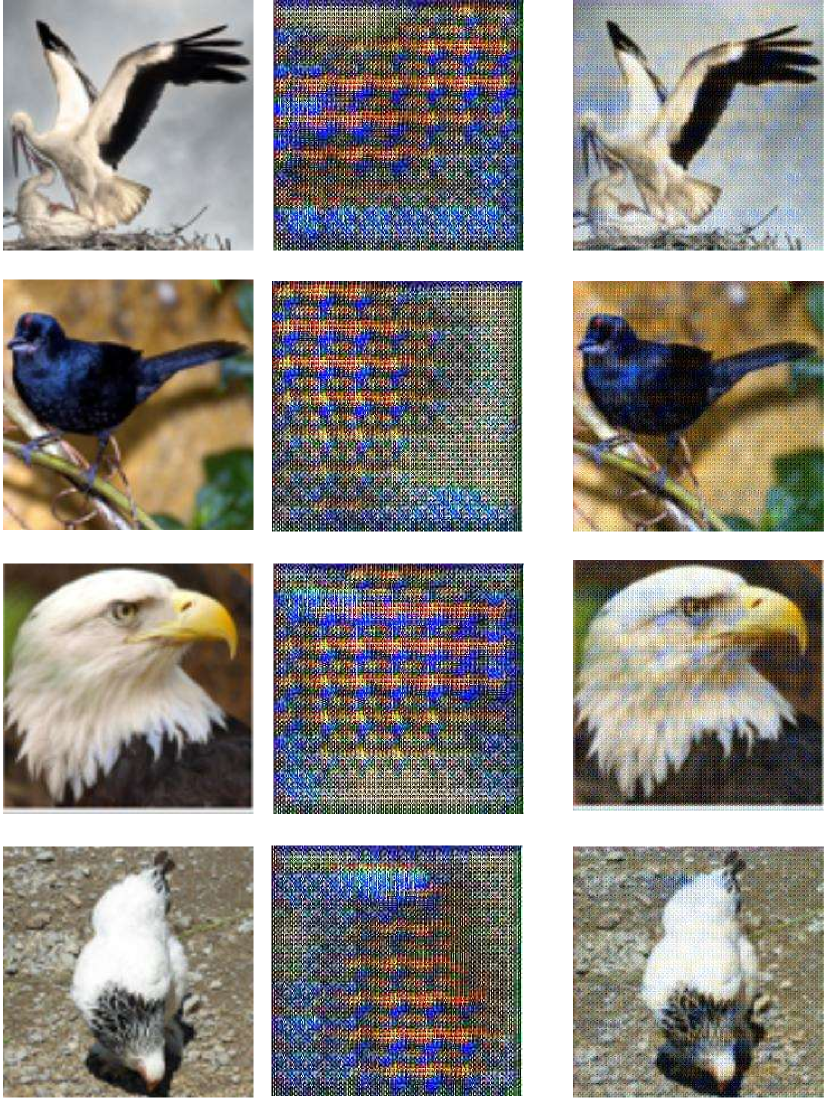
(B)

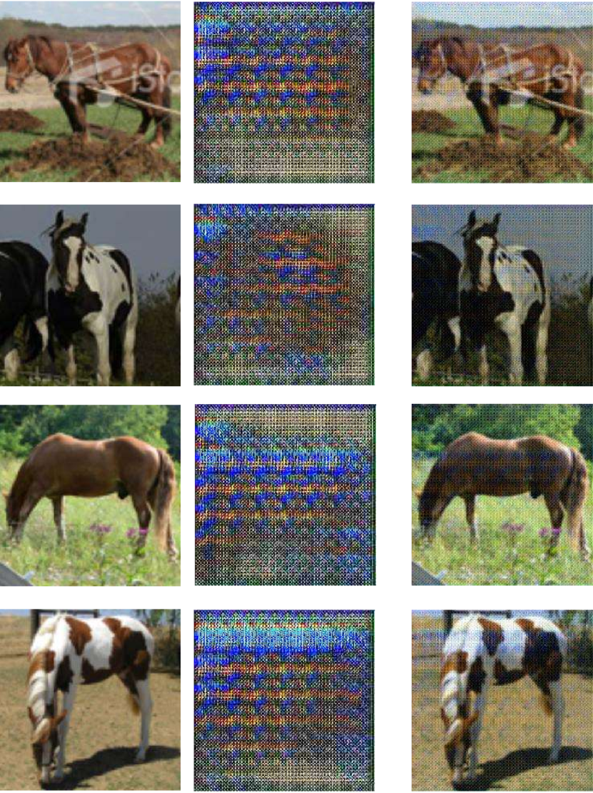
(C)

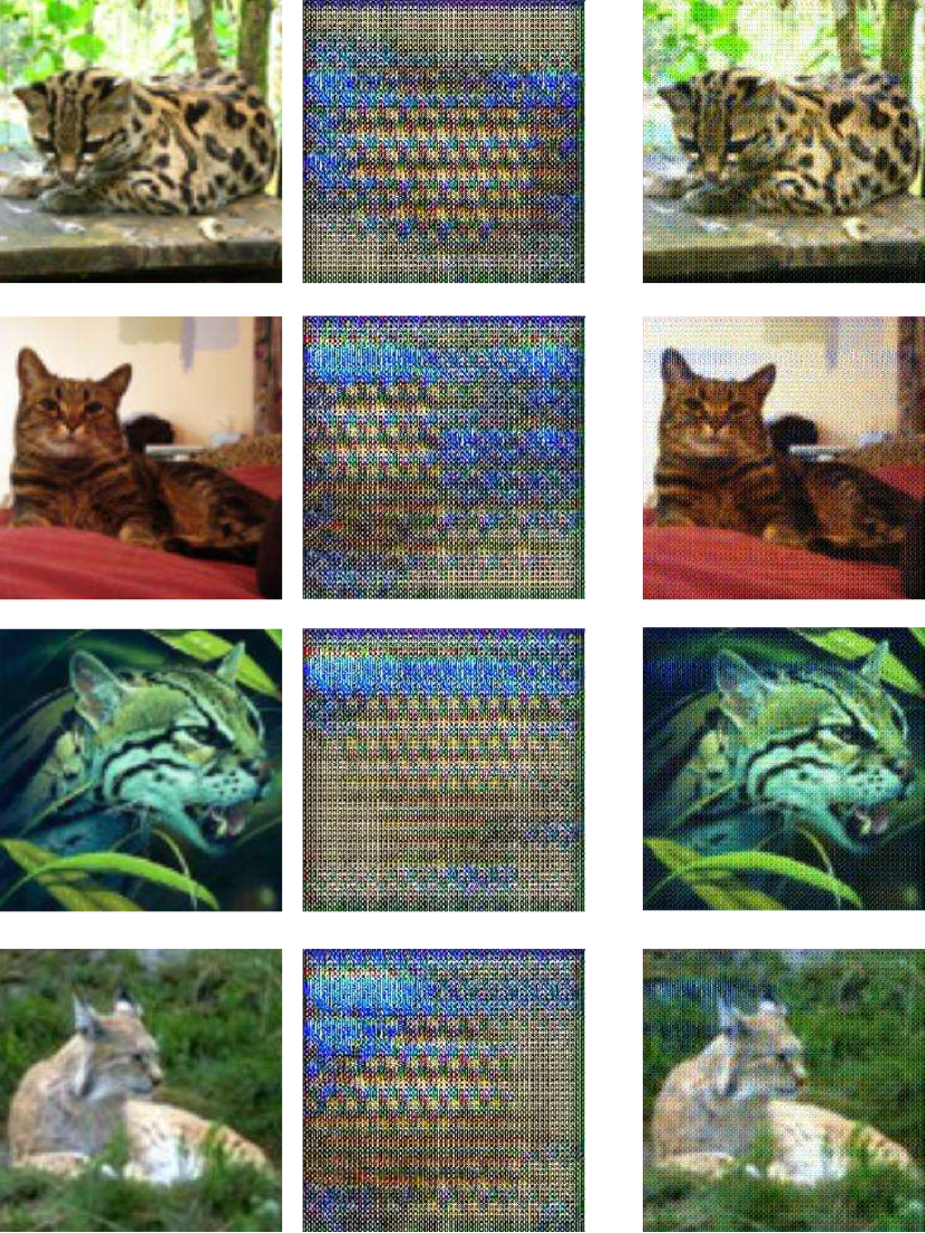
(D)

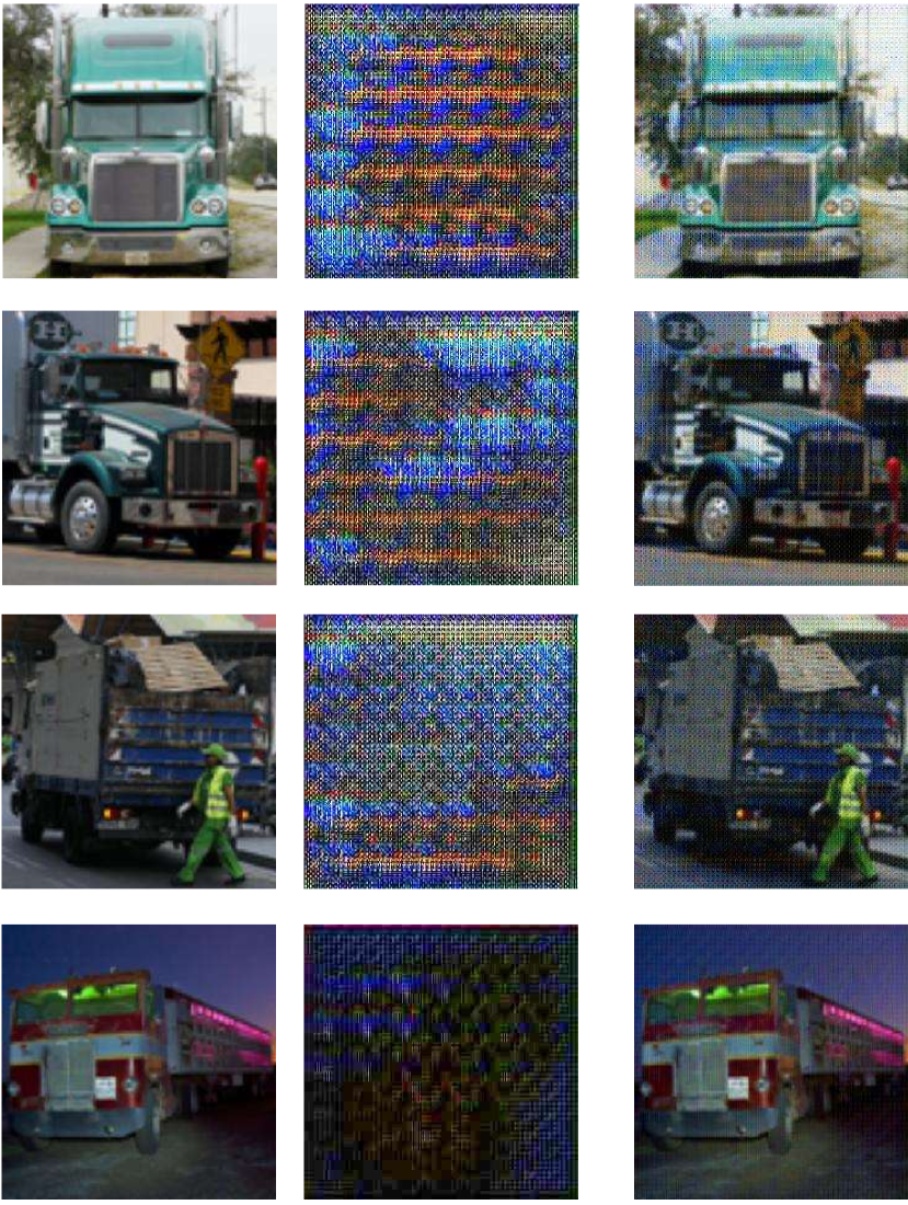
Figure 13: Examples of generated perturbation from non-normalized images in diverse image classes for performance enhancement problem. (A) eagle, (B) horse, (C) cat, and (D) truck.

In Figures 11, 12, 13, and 14, additional perturbations and corresponding perturbed images for diverse image classes are presented. The perturbations in Figures 11, 12 were generated from normalized images, and those in Figures 13, and 14 were generated from non-normalized images. Figures 11 and 13 show the examples of performance enhancement problem, and Figures 12 and 14 present the examples of performance degradation problem. It is interesting that the perturbations for each image class seem to share some similar visual characteristics among them when seeing Figure 11. For example, the perturbations generated from ‘fox’ images and that from ‘bug’ images have clearly discriminative shapes from each other.

(A)

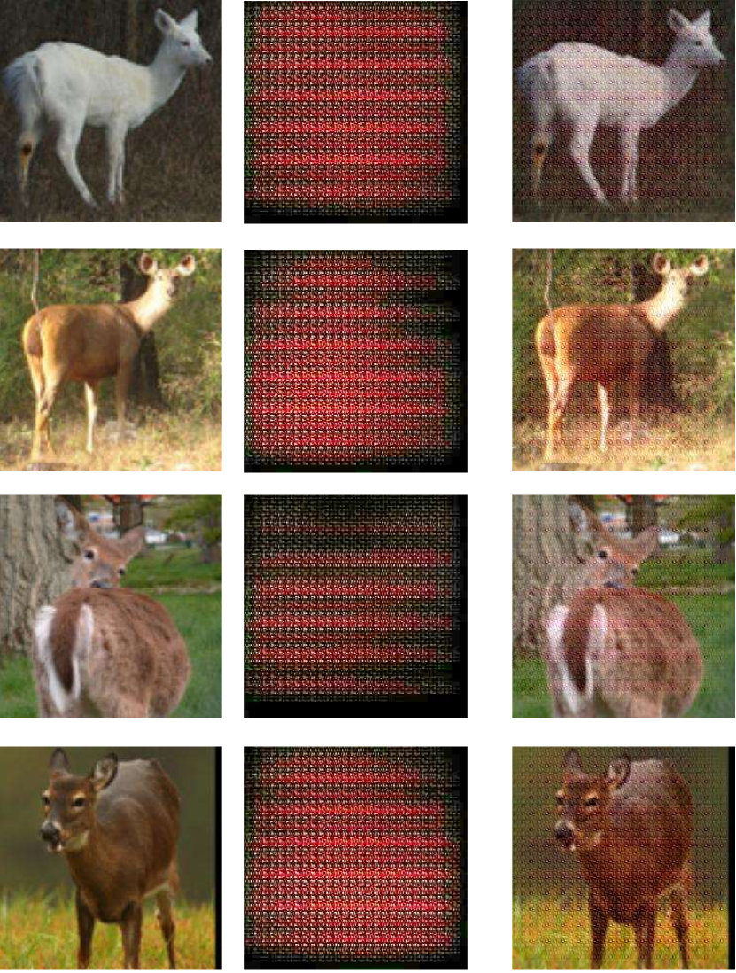
(B)

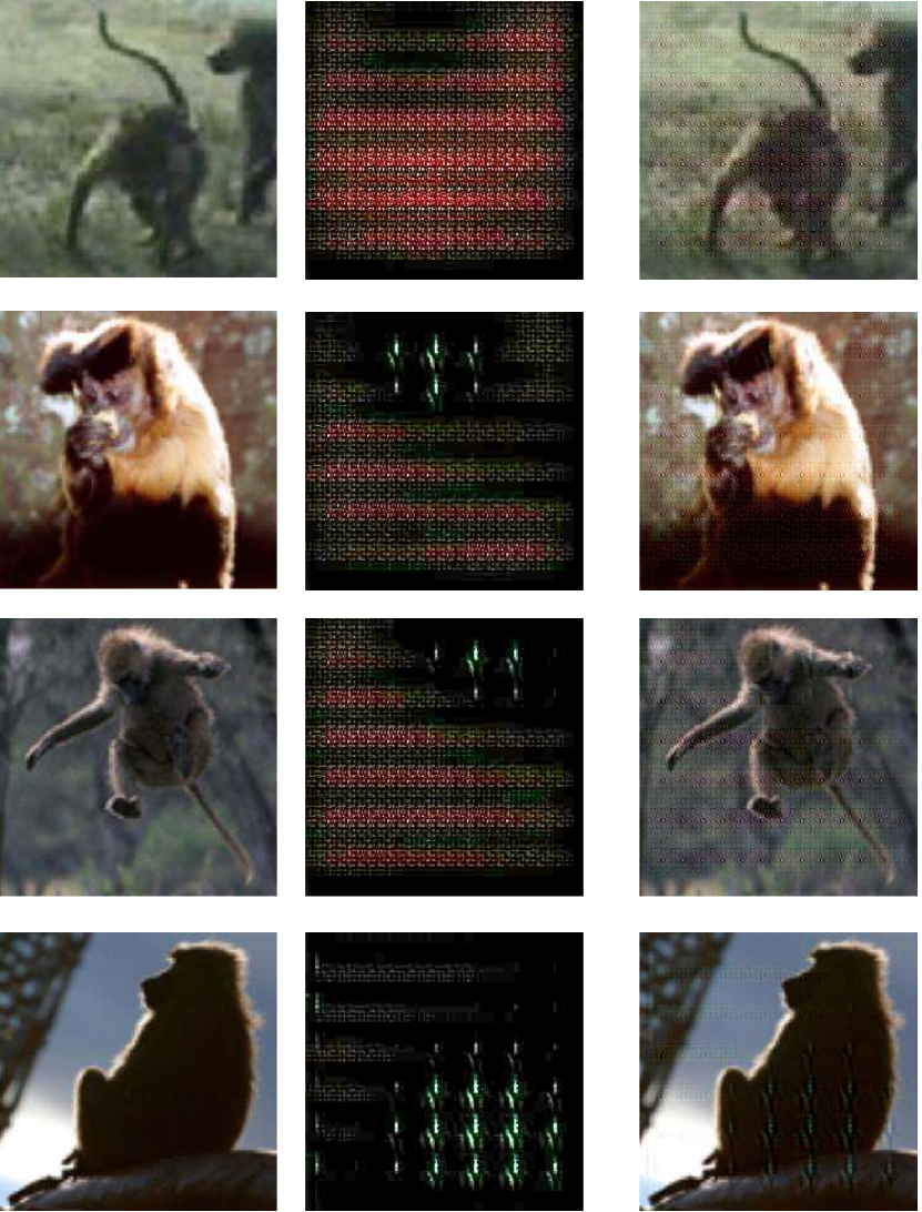
(C)

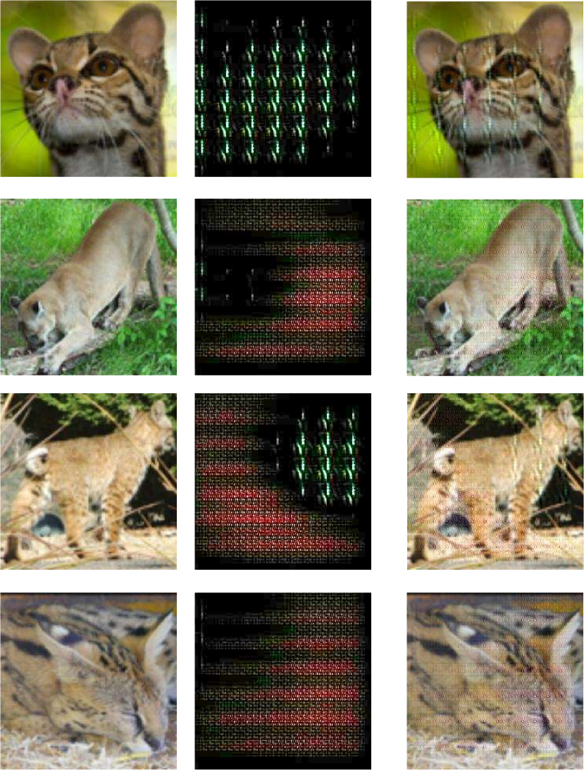
(D)

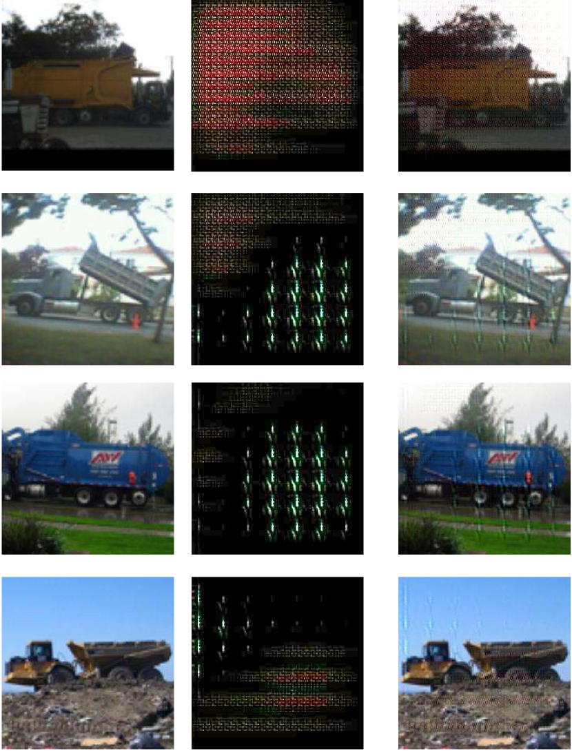
Figure 14: Examples of generated perturbation from non-normalized images in diverse image classes for performance degradation problem. (A) deer, (B) monkey, (C) cat, and (D) truck.

References

- [1] S. Baluja and I. Fischer. Adversarial transformation networks: Learning to generate adversarial examples. arXiv preprint arXiv:1703.09387, 2017.
- [2] O. Bastani, Y. Ioannou, L. Lampropoulos, D. Vytiniotis, A. Nori, and A. Criminisi. Measuring neural net robustness with constraints. In Advances in Neural Information Processing Systems, pages 2613–2621, 2016.
- [3] B. Biggio, I. Corona, D. Maiorca, B. Nelson, N. Šrndić, P. Laskov, G. Giacinto, and F. Roli. Evasion attacks against machine learning at test time. In Joint European Conference on Machine Learning and Knowledge Discovery in Databases, pages 387–402. Springer, 2013.
- [4] J. Bradshaw, A. G. d. G. Matthews, and Z. Ghahramani. Adversarial examples, uncertainty, and transfer testing robustness in gaussian process hybrid deep networks. arXiv preprint arXiv:1707.02476, 2017.
- [5] A. Coates, A. Ng, and H. Lee. An analysis of single-layer networks in unsupervised feature learning. In Proceedings of the fourteenth international conference on artificial intelligence and statistics, pages 215–223, 2011.
- [6] N. Das, M. Shanbhogue, S.-T. Chen, F. Hohman, L. Chen, M. E. Kounavis, and D. H. Chau. Keeping the bad guys out: Protecting and vaccinating deep learning with jpeg compression. arXiv preprint arXiv:1705.02900, 2017.
- [7] A. Fawzi, O. Fawzi, and P. Frossard. Analysis of classifiers’ robustness to adversarial perturbations. arXiv preprint arXiv:1502.02590, 2015.
- [8] A. Fawzi, S.-M. Moosavi-Dezfooli, and P. Frossard. Robustness of classifiers: from adversarial to random noise. In Advances in Neural Information Processing Systems, pages 1632–1640, 2016.
- [9] R. Girshick. Fast r-cnn. In Proceedings of the IEEE international conference on computer vision, pages 1440–1448, 2015.
- [10] I. Goodfellow, J. Pouget-Abadie, M. Mirza, B. Xu, D. Warde-Farley, S. Ozair, A. Courville, and Y. Bengio. Generative adversarial nets. In Advances in neural information processing systems, pages 2672–2680, 2014.
- [11] I. J. Goodfellow, J. Shlens, and C. Szegedy. Explaining and harnessing adversarial examples. arXiv preprint arXiv:1412.6572, 2014.
- [12] S. Gu and L. Rigazio. Towards deep neural network architectures robust to adversarial examples. arXiv preprint arXiv:1412.5068, 2014.
- [13] J. Hayes and G. Danezis. Machine learning as an adversarial service: Learning black-box adversarial examples. arXiv preprint arXiv:1708.05207, 2017.
- [14] K. He, X. Zhang, S. Ren, and J. Sun. Deep residual learning for image recognition. In Proceedings of the IEEE conference on computer vision and pattern recognition, pages 770–778, 2016.
- [15] H. Hosseini, Y. Chen, S. Kannan, B. Zhang, and R. Poovendran. Blocking transferability of adversarial examples in black-box learning systems. arXiv preprint arXiv:1703.04318, 2017.
- [16] G. Huang, Z. Liu, K. Q. Weinberger, and L. van der Maaten. Densely connected convolutional networks. arXiv preprint arXiv:1608.06993, 2016.
- [17] D. Kingma and J. Ba. Adam: A method for stochastic optimization. arXiv preprint arXiv:1412.6980, 2014.
- [18] A. Krizhevsky, I. Sutskever, and G. E. Hinton. Imagenet classification with deep convolutional neural networks. In Advances in neural information processing systems, pages 1097–1105, 2012.
- [19] Y. LeCun, B. Boser, J. S. Denker, D. Henderson, R. E. Howard, W. Hubbard, and L. D. Jackel. Backpropagation applied to handwritten zip code recognition. Neural computation, 1(4):541–551, 1989.
- [20] Y. Liu, X. Chen, C. Liu, and D. Song. Delving into transferable adversarial examples and black-box attacks. arXiv preprint arXiv:1611.02770, 2016.
- [21] J. Long, E. Shelhamer, and T. Darrell. Fully convolutional networks for semantic segmentation. In Proceedings of the IEEE Conference on Computer Vision and Pattern Recognition, pages 3431–3440, 2015.
- [22] J. Lu, T. Issaranon, and D. Forsyth. Safetynet: Detecting and rejecting adversarial examples robustly. arXiv preprint arXiv:1704.00103, 2017.
- [23] J. Lu, H. Sibai, E. Fabry, and D. Forsyth. No need to worry about adversarial examples in object detection in autonomous vehicles. arXiv preprint arXiv:1707.03501, 2017.
- [24] X. Mao, Q. Li, H. Xie, R. Y. Lau, Z. Wang, and S. P. Smolley. Least squares generative adversarial networks. arXiv preprint ArXiv:1611.04076, 2016.
- [25] J. H. Metzen, T. Genewein, V. Fischer, and B. Bischoff. On detecting adversarial perturbations. arXiv preprint arXiv:1702.04267, 2017.
- [26] S.-M. Moosavi-Dezfooli, A. Fawzi, O. Fawzi, and P. Frossard. Universal adversarial perturbations. In The IEEE Conference on Computer Vision and Pattern Recognition (CVPR), July 2017.
- [27] S.-M. Moosavi-Dezfooli, A. Fawzi, O. Fawzi, P. Frossard, and S. Soatto. Analysis of universal adversarial perturbations. arXiv preprint arXiv:1705.09554, 2017.
- [28] S.-M. Moosavi-Dezfooli, A. Fawzi, and P. Frossard. Deepfool: a simple and accurate method to fool deep neural networks. In Proceedings of the IEEE Conference on Computer Vision and Pattern Recognition, pages 2574–2582, 2016.
- [29] K. R. Mopuri, U. Garg, and R. V. Babu. Fast feature fool: A data independent approach to universal adversarial perturbations. arXiv preprint arXiv:1707.05572, 2017.
- [30] A. Mordvintsev, C. Olah, and M. Tyka. Deepdream-a code example for visualizing neural networks. Google Res, 2015.
- [31] A. Nguyen, J. Yosinski, and J. Clune. Deep neural networks are easily fooled: High confidence predictions for unrecognizable images. In Proceedings of the IEEE Conference on Computer Vision and Pattern Recognition, pages 427–436, 2015.
- [32] H. Noh, S. Hong, and B. Han. Learning deconvolution network for semantic segmentation. In Proceedings of the IEEE International Conference on Computer Vision, pages 1520–1528, 2015.
- [33] S. J. Oh, M. Fritz, and B. Schiele. Adversarial image perturbation for privacy protection–a game theory perspective. arXiv preprint arXiv:1703.09471, 2017.
- [34] T. Orekondy, B. Schiele, and M. Fritz. Towards a visual privacy advisor: Understanding and predicting privacy risks in images. arXiv preprint arXiv:1703.10660, 2017.
- [35] A. Radford, L. Metz, and S. Chintala. Unsupervised representation learning with deep convolutional generative adversarial networks. arXiv preprint arXiv:1511.06434, 2015.
- [36] J. Redmon, S. Divvala, R. Girshick, and A. Farhadi. You only look once: Unified, real-time object detection. In Proceedings of the IEEE Conference on Computer Vision and Pattern Recognition, pages 779–788, 2016.
- [37] S. Ren, K. He, R. Girshick, and J. Sun. Faster r-cnn: Towards real-time object detection with region proposal networks. In Advances in neural information processing systems, pages 91–99, 2015.
- [38] E. Rodner, M. Simon, R. B. Fisher, and J. Denzler. Fine-grained recognition in the noisy wild: Sensitivity analysis of convolutional neural networks approaches. arXiv preprint arXiv:1610.06756, 2016.
- [39] A. Rozsa, E. M. Rudd, and T. E. Boult. Adversarial diversity and hard positive generation. In Proceedings of the IEEE Conference on Computer Vision and Pattern Recognition Workshops, pages 25–32, 2016.
- [40] O. Russakovsky, J. Deng, H. Su, J. Krause, S. Satheesh, S. Ma, Z. Huang, A. Karpathy, A. Khosla, M. Bernstein, et al. Imagenet large scale visual recognition challenge. International Journal of Computer Vision, 115(3):211–252, 2015.
- [41] S. Sabour, Y. Cao, F. Faghri, and D. J. Fleet. Adversarial manipulation of deep representations. arXiv preprint arXiv:1511.05122, 2015.
- [42] K. Simonyan and A. Zisserman. Very deep convolutional networks for large-scale image recognition. arXiv preprint arXiv:1409.1556, 2014.
- [43] C. Szegedy, S. Ioffe, V. Vanhoucke, and A. A. Alemi. Inception-v4, inception-resnet and the impact of residual connections on learning. In AAAI, pages 4278–4284, 2017.
- [44] C. Szegedy, W. Liu, Y. Jia, P. Sermanet, S. Reed, D. Anguelov, D. Erhan, V. Vanhoucke, and A. Rabinovich. Going deeper with convolutions. In Proceedings of the IEEE conference on computer vision and pattern recognition, pages 1–9, 2015.
- [45] C. Szegedy, W. Zaremba, I. Sutskever, J. Bruna, D. Erhan, I. Goodfellow, and R. Fergus. Intriguing properties of neural networks. arXiv preprint arXiv:1312.6199, 2013.
- [46] P. Tabacof and E. Valle. Exploring the space of adversarial images. In Neural Networks (IJCNN), 2016 International Joint Conference on, pages 426–433. IEEE, 2016.
- [47] T. Tieleman and G. Hinton. Lecture 6.5-rmsprop: Divide the gradient by a running average of its recent magnitude. COURSERA: Neural networks for machine learning, 4(2):26–31, 2012.
- [48] C. Xie, J. Wang, Z. Zhang, Y. Zhou, L. Xie, and A. Yuille. Adversarial examples for semantic segmentation and object detection. arXiv preprint arXiv:1703.08603, 2017.
- [49] V. Zantedeschi, M.-I. Nicolae, and A. Rawat. Efficient defenses against adversarial attacks. arXiv preprint arXiv:1707.06728, 2017.