Parameterizations of Chromospheric Condensations in dG and dMe Model Flare Atmospheres

Abstract

The origin of the near-ultraviolet and optical continuum radiation in flares is critical for understanding particle acceleration and impulsive heating in stellar atmospheres. Radiative-hydrodynamic simulations in 1D have shown that high energy deposition rates from electron beams produce two flaring layers at $T\sim 10^{4}$ K that develop in the chromosphere: a cooling condensation (downflowing compression) and heated non-moving (stationary) flare layers just below the condensation. These atmospheres reproduce several observed phenomena in flare spectra, such as the red wing asymmetry of the emission lines in solar flares and a small Balmer jump ratio in M dwarf flares. The high beam flux simulations are computationally expensive in 1D, and the (human) timescales for completing NLTE models with adaptive grids in 3D will likely be unwieldy for a time to come. We have developed a prescription for predicting the approximate evolved states, continuum optical depth, and the emergent continuum flux spectra of radiative-hydrodynamic model flare atmospheres. These approximate prescriptions are based on an important atmospheric parameter: the column mass ($m_{\rm{ref}}$) at which hydrogen becomes nearly completely ionized at the depths that are approximately in steady state with the electron beam heating. Using this new modeling approach, we find that high energy flux density ($>$F11) electron beams are needed to reproduce the brightest observed continuum intensity in IRIS data of the 2014-Mar-29 X1 solar flare and that variation in $m_{\rm{ref}}$ from 0.001 to 0.02 g cm^-2 reproduces most of the observed range of the optical continuum flux ratios at the peaks of M dwarf flares.

1 Introduction

Stellar flares are thought to be produced from the atmospheric heating that results from coronal magnetic field reconnection and retraction. Ambient electrons, protons, and heavy nuclei are accelerated to very high energies and produce the observed X-ray and gamma-ray emissions. The hard X-ray emission at tens to hundreds of keV is cospatial and cotemperal with typical signatures of chromospheric heating, such as H$\alpha$ ribbons and the near-ultraviolet (NUV; $\lambda=2000-4000$ Å) and optical ($\lambda=4000-7000$ Å) continuum radiation. Thus, these high energy particles are likely the source of powering most of the chromospheric heating and radiative response. Moreover, recent high spatial resolution imagery of NUV and optical footpoints in solar flares suggest a very high electron beam flux density (Fletcher et al., 2007; Krucker et al., 2011; Kleint et al., 2016; Jing et al., 2016; Kowalski et al., 2017a; Sharykin et al., 2017) which may be difficult to sustain due to plasma instabilities (Lee et al., 2008; Li et al., 2014).

Radiative-hydrodynamic (RHD) simulations with heating from high beam flux densities nonetheless provide important insights into the atmospheric response that produces several well-observed spectral phenomena in M dwarf and solar flares. A high flux density of nonthermal electrons with a low energy cutoff of $E_{c}=20-40$ keV produces dense, downflowing compressions that originate in the mid to upper chromosphere. These chromospheric compressions (or chromospheric condensations, hereafter “CC”s) have physical depth ranges in the atmosphere of $\Delta z\sim 20-30$ km. The CCs evolve from high temperature and low density to low temperature ($T\sim$10,000 K) and much higher density as they compress and descend to the lower chromosphere (Kennedy et al., 2015; Kowalski et al., 2015); most of the CC evolution occurs on timescales of seconds to several tens of seconds (Fisher, 1989); CCs have been extensively modeled in the literature (Livshits et al., 1981; Emslie & Nagai, 1985; Fisher et al., 1985b, a; Canfield & Gayley, 1987; Gan et al., 1992).

In solar flares, compelling observational evidence exists for the formation of these CCs. The spectrally resolved red-wing asymmetry (often referred to as “RWA”) in chromospheric lines such as H$\alpha$, Mg II, and Fe II is frequently observed in the impulsive phase of flares (Ichimoto & Kurokawa, 1984; Graham & Cauzzi, 2015; Kowalski et al., 2017a). These RWAs exhibit spectrally resolved peaks with redshifts of $\lambda-\lambda_{\rm{rest}}=15-140$ km s^-1. The brightness of the RWA in NUV Fe II lines relative to the intensity of the line component at the rest wavelength has been reproduced with a high flux electron beam of 5x10¹¹ erg cm^-2 s^-1 (hereafter, 5F11; Kowalski et al., 2017a).

In magnetically active M dwarf (dMe) flares, the observed NUV and optical flare continuum (sometimes referred to as white-light radiation if detected in broadband optical radiation on the Sun or in the Johnson $U$-band in dMe stars) distribution can be reproduced in 1D model snapshots of a very dense, evolved CC that results from the extremely high energy flux density ($\sim 10^{13}$ erg cm^-2 s^-1, hereafter F13) in nonthermal electron beams lasting several seconds (Kowalski et al., 2015, 2016, 2017b). This flux density is expected to result in beam instabilities (even in the much larger ambient coronal densities of dMe stars) and a strong return current electric field (e.g., van den Oord, 1990). Also, the hydrogen Balmer line broadening predicted from these evolved CCs far exceeds the typical values that are observed without including several other lower density emitting regions in the modeling (Kowalski et al., 2017b). Alternative heating scenarios may be necessary to reproduce the continuum radiation, such as a very high low-energy cutoff (Kowalski et al., 2017b), high energy proton/ion beams, or possibly Alfven wave heating (Reep & Russell, 2016; Kerr et al., 2016). Only a limited range of heating simulations with electron beam flux densities between $\sim 10^{12}$ and $\sim 10^{13}$ erg cm^-2 s^-1 has been tested to determine if such a high beam density of $\sim 10^{13}$ erg cm^-2 s^-1 is required to produce the observed range of flare continuum flux ratios and Balmer line broadening in dMe flares.

The atmospheric response to the energy deposition from a high beam flux density of nonthermal electrons results in complete helium ionization and a thermal instability as the temperature exceeds the peak of the radiative loss function for C and O ions at $T\sim 100,000-200,000$ K. The chromospheric temperature initially at $T\sim 7000$ K exceeds 10 MK in less than a fraction of a second after beam heating begins; this localized explosion in the chromosphere results in large temperature, density, pressure, and ionization fraction changes over very narrow height ranges, $\Delta z\sim 10-15$ meters. One-dimensional RHD simulations have the advantage of resolving these gradients with an adaptive grid (Dorfi & Drury, 1987), but the atmospheric evolution can take weeks to several months to compute (Abbett & Hawley, 1999; Allred et al., 2005, 2006; Kowalski et al., 2015; Kennedy et al., 2015). The small time steps ($10^{-7}-10^{-8}$ s) in these calculations are caused by the accuracy of the helium population convergence at these steep gradients and are exacerbated by a radiative instability in a very narrow ($\sim 5$ km), cool region between the flare corona and the large temperature gradient at the chromospheric explosion (see Kennedy et al., 2015). The onset threshold of explosive evaporation and condensation in the chromosphere depends upon all of the parameters that characterize electron beam heating (Fisher, 1989) but generally occurs at high energy flux densities, typically exceeding $10^{11}$ erg cm^-2 s^-1 (F11) with a moderate low-energy cutoff $E_{\rm{c}}$ value ($E_{\rm{c}}\sim 25$ keV; Kowalski et al., 2017a).

There are far less constraints on the electron beam parameters in dMe flares because the hard X-ray flux is faint except during extreme events; in these events, the hard X-ray emission can be explained by a superhot thermal component (Osten et al., 2007, 2010, 2016). Radio observations directly probe mildly relativistic electrons in dMe flares, but one must observe at optically thin frequencies in order to relate the power law index of the radio emission directly to the power law index of electrons (Dulk, 1985; Osten et al., 2005; Smith et al., 2005; Osten et al., 2016). Due to the large contrast at NUV and blue optical wavelengths, flare spectra around the Balmer limit wavelength are the most direct way to probe the impulsive release of magnetic energy in dMe flares. Models over a large parameter space of electron beam heating can then be used to infer the properties of the accelerated particles in these very active stars. Large grids of models would also show if very high beam flux densities ($\sim$F13) are required to produce the observed spectral properties in dMe flares. This would motivate improving the treatment of electron beam propagation to include the effects of the return current electric field and plasma instabilities.

Modeling the full RHD response even in 1D for a large parameter space of electron beam distributions with very high heating rates is currently computationally challenging and will become more time-consuming when 3D models that employ adaptive grids for resolving steep pressure gradients are developed in the future. In this paper, we present a method for obtaining prompt insight into the evolution of the radiative and hydrodynamic response to high energy deposition rates from electron beams with a low-to-moderate low-energy cutoff ($E_{c}=15-40$ keV), thus providing important guidance about which heating models are most interesting to follow with RADYN for the full evolution. This paper is organized as follows: In section 2.1 we summarize the response to high electron beam flux densities in solar and dMe atmospheres that are used in the analysis, in section 2.2 we describe our analysis and prescription for approximating the RHD models of the evolved states of these flare atmospheres, in section 3 we discuss several applications for our approximate model atmospheres, and in section 4 we present several new conclusions about flares that are based off of our approximations. In an appendix, we show that our new modeling prescriptions can be used to produce broad wavelength flare spectral predictions.

2 Approximations to Dynamic Flare Atmospheres

2.1 High Beam Flux Density RHD Modeling with the RADYN Code

High electron beam flux density simulations with a low-energy cutoff of $E_{c}=20-40$ keV produce two dense layers at low temperature ($T\lesssim 13,000$ K) at pre-flare chromospheric heights which flare brightly in NUV and optical radiation (Kowalski et al., 2015, 2016; Kowalski, 2016; Kowalski et al., 2017a). The electron beam distribution is characterized by a power-law index, and most of the beam energy is thus concentrated near the low-energy cutoff. The two flaring layers that develop from high energy deposition rates in the mid to upper chromosphere are the following:

1. A downflowing ($v\sim 50-100$ km s^-1), hot ($T\sim 10,000-13,000$ K) and dense (several x $10^{14}$ to several x$10^{15}$ cm^-3) region that is several tens of km in vertical extent just below a lower steep pressure/temperature gradient; this region is the CC, which increases in density and cools as it accretes more material and slows during its descent to the lower chromosphere. The energy deposition within the CC is due to intermediate energy electrons in the beam. Beam electrons at the low energy cutoff produce and heat the localized temperature increase in the chromosphere to $T=5-10$ MK.

2. The layers below the CC can also be significantly heated by the high energy electrons in the beam ($E>>E_{\rm{c}}$ keV); this region is referred to as the stationary flare layers because it exhibits negligible ($\lesssim 1$ km s^-1 upward) gas velocities relative to the CC. The stationary flare layers extend several hundred km below the CC and are $T\sim 9000-12,000$ K, which is less than the temperature range in the CC during its early evolution.

In Figure 1, we illustrate these two flaring layers that develop in response to heating by high flux density electron beams.

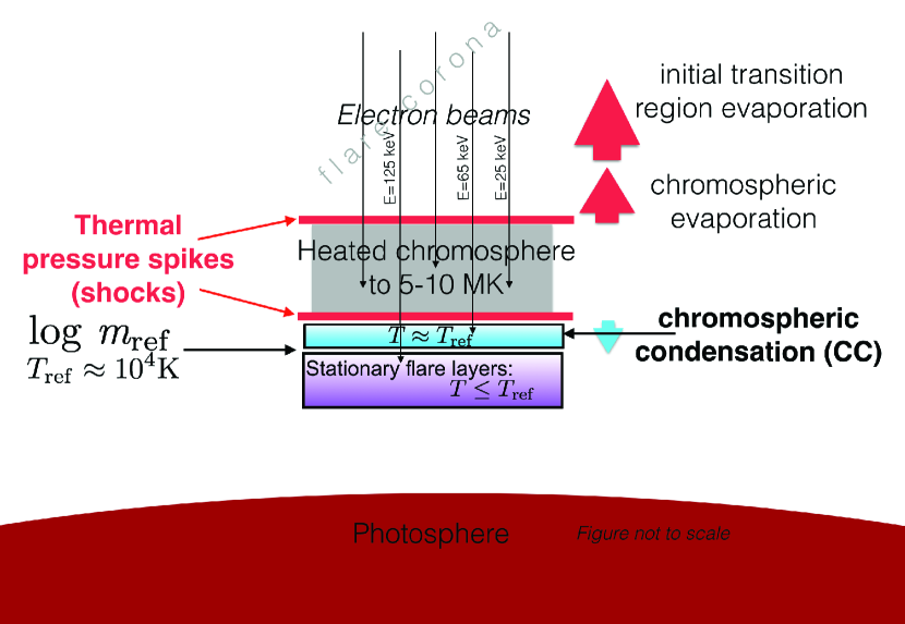
Figure 1: Cartoon illustrating the important features that develop in the evolved atmospheric states with high beam flux heating rates. The height corresponding to log $m_{\rm{ref}}$ and $T_{\rm{ref}}$ occurs at the interface between the dense, downflowing cool ($T\approx 10^{4}$ K) chromospheric condensation and heated stationary flare layers (note that by the evolved-1 time, the temperature at $m_{\rm{ref}}$ has increased to approximately $T_{\rm{ref}}+1500$ K for the very high beam flux density F13 models). Thick colored arrows indicate plasma motions that have developed by the evolved times. The approximate stopping depths for representative low (25 keV), intermediate (65 keV) and high energy (125 keV) beam electrons in the 5F11$\_$soft$\_$sol model are indicated (black thin arrows) using the thick target formulae of Emslie (1978, 1981), Ricchiazzi & Canfield (1983), and Hawley & Fisher (1994) corrected for relativistic length contraction (Allred et al., 2015). For the F13$\_$soft$\_$dMe model, representative electron beam energies for these arrows are 65 keV, 125 keV and 300 keV, respectively. Features in this figure have been adapted from Kowalski (2016).

With extremely high beam energy flux densities ($\sim$F13), these two flaring regions develop an optical depth $\tau>1$ at NUV and optical continuum wavelengths, and the emergent radiation is characterized by a hot $T\sim 10^{4}$ K blackbody-like spectrum with a small Balmer jump ratio, as observed in spectral, broadband photometric, and narrowband photometric observations of dMe flares (Hawley & Pettersen, 1991; Zhilyaev et al., 2007; Fuhrmeister et al., 2008; Kowalski et al., 2013). If the beam energy flux densities are moderately high ($\sim$5F11), then bright NUV continuum intensity and Fe II emission lines are produced with a prominent red wing asymmetry, as observed in NUV (at $\lambda\sim 2830$ Å) solar flare spectra from IRIS.

Only after several seconds of high beam flux heating do these interesting properties develop in these simulations. In this paper, we parameterize the temperature and density stratification of these RADYN simulations at the advanced states in order to make predictions and some general conclusions about the emergent continuum radiation spectrum over a large possible range of conditions in chromospheric condensations. This will allow us (in future work) to select and run an interesting subset of RHD simulations based off of information at early times in order to make detailed line profile calculations at the evolved states of the simulations.

In the few high beam flux density simulations that have been completed with RADYN, we have noticed common patterns in their evolved states. In this paper, these patterns are used for parameterizations of the evolved states of the temperature and density stratifications. The high beam flux density simulations that we use in this analysis are the 5F11 (extended heating run; “5F11$\_$soft$\_$sol”) solar flare model from Kowalski et al. (2017a), the F13 dMe flare model with a double-power (“F13$\_$soft$\_$dMe”) distribution of electron energy (Kowalski et al., 2015), and the F13 dMe flare model with a harder single power law distribution (“F13$\_$hard$\_$dMe”) of electron energy with a power-law index of $\delta=3$ (Kowalski et al., 2016). The model parameters are summarized in Table 1. The distinction between hard and soft beams is made according to the relative number of nonthermal electrons at $E\gtrsim 200$ keV, which are important for the heating and ionization in the stationary flare layers (Kowalski et al., 2016). These RHD calculations were performed with the 1D RHD RADYN code (Carlsson & Stein, 1992, 1994, 1995, 1997, 2002), which calculates hydrogen, helium, and Ca II in NLTE and with non-equilibrium ionization/excitation (NEI). We refer the reader to Allred et al. (2015), Kowalski et al. (2015), and Kowalski et al. (2017a) for extensive descriptions of the flare simulations.

For each simulation, we analyze the atmospheric states at an “early” time and two “evolved” times in Table 1. The early times correspond to the early development of the CC when it exhibits a temperature of $T\sim 40,000$ K and is flowing downward at approximately its maximum downflow speed; this time also corresponds to when the stationary flare layers have achieved a temperature stratification that is relatively constant at any later time. These conditions occur when the explosive temperature shock front in the chromosphere exceeds $T=2.5$ MK in the 5F11$\_$soft$\_$sol and $T=10$ MK in the F13 models. We choose $t=1.2$ s as the best time to represent the early state of the 5F11$\_$soft$\_$sol model and $t=0.4$ s to represent the early states of the F13 models.

The evolved times (“evolved-1” and “evolved-2”) in each simulation correspond to the times when the CC has cooled to $T\sim 9000-13,000$ K and the stationary flare layers have heated to a similar temperate range. At the evolved times in each simulation, the flare atmospheres produce the brightest optical and NUV continuum and line radiation as well as the largest continuum optical depth.

Two evolved states in each RADYN simulation are considered to represent a range of possible extreme conditions that can be achieved. For the F13$\_$soft$\_$dMe model, the minimum temperature in the CC has decreased to $T\sim 13,000$ K at $t=1.6$ s, which is also the time of the maximum emergent continuum intensity at wavelengths just shortward of the Balmer limit ($\lambda=3646$ Å). We refer to $t=1.6$ s as the evolved-1 time for the F13$\_$soft$\_$dMe. However, the Balmer jump ratio continues to decrease to $t=2.2$ s as the CC accrues more material as it cools, resulting in a decrease of the physical depth range over which $\lambda=3500$ Å photons escape (see Kowalski et al., 2015). At this point the blue $\lambda=4170$ Å photons still escape from the stationary flare layers due to a lower optical depth in the CC $\tau_{4170}(\rm{CC})<1$. The time of $t=2.2$ s is the evolved-2 time for the F13$\_$soft$\_$dMe. In the F13$\_$hard$\_$dMe simulation the CC cools to $T\sim 13,000$ K at the evolved-1 time of $t=2.2$ s; the evolved-2 time is not attained before the heating ceases at $t=2.3$ s.

For the 5F11$\_$soft$\_$sol model, the evolved-1 time is $t=3.97$ s, which was analyzed extensively in Kowalski et al. (2017a) and results in nearly the brightest NUV continuum intensity as the minimum temperature in the CC decreases to $T=10,000$ K. The evolved-2 time corresponds to the maximum NUV continuum intensity at $t=5$ s.

The timescales for CC development in these high beam flux heating models are similar to the most recent observational constraints (several seconds to twenty seconds; Penn et al., 2016; Rubio da Costa et al., 2016) of electron beam heating duration in a single flare loop. Therefore, the two evolved times bracket the possible range of atmospheric conditions, NUV continuum intensity, and NUV continuum optical depth in order to account for the uncertainty in the duration of flare heating in a loop. In summary, the evolved-1 times correspond to when the minimum temperature in the CC cools to $T\sim 13,000$ K in high beam flux simulations and $T\sim 10,000$ K in lower beam flux simulations. The evolved-2 times correspond to further development of the CC at $\Delta t=0.6$ s after the evolved-1 time in very high (F13) beam flux simulations and at $\Delta t=1$ s after the evolved-1 time in lower (5F11) beam flux simulations.

Table 1: Model Parameters

RADYN Model	Flux density	Heating duration (s)	log $g$	Power-law index ($\delta$)	Low energy cutoff (keV)	Early Time (s)	Evolved-1 Time (s)	Evolved-2 Time (s)
5F11$\_$soft$\_$sol	$5\times 10^{11}$	15	4.44	$4.2$	25	1.2	3.97	5.0
F13$\_$soft$\_$dMe	$10^{13}$	2.3	4.75	$3,4$	37	0.4	1.6	2.2
F13$\_$hard$\_$dMe	$10^{13}$	2.3	4.75	$3$	37	0.4	2.2	–

Note. — Basic information about the electron beam models and the times designated as the early, evolved-1, evolved-2 times for each. The double power-law F13 model has power-law indices of $\delta=3$ at $E<105$ keV and $\delta=4$ at $E>105$ keV. The flux density above $E_{\rm{cutoff}}$ is given in units of erg cm^-2 s^-1.

2.2 The Critical Flare Atmosphere Reference Parameters

We use the 5F11$\_$soft$\_$sol solar flare simulation to construct a simplified, approximate parameterization of the thermodynamic stratifications at the evolved-1 and evolved-2 times ($t=3.97$ s and 5 s, respectively) using only two reference atmospheric quantities in the RADYN calculation at the early time ($t=1.2$ s).

Figure 2 shows the temperature evolution of the 5F11$\_$soft$\_$sol model from $t=0-3.97$ s. After the early time of $t=$1.2 s, the atmospheric temperature structure in the stationary flare layers at column mass $m$ larger than log $m\gtrsim-2.75$ (corresponding to the vertical dashed blue line) does not change significantly (i.e., the thick black and thick red solid lines are similar at larger column mass than log $m\gtrsim-2.75$). In the 5F11$\_$soft$\_$sol simulation, the lower pressure gradient at the temperature explosion to $T=2.5-5$ MK compresses the gas that is initially spread over a physical depth range of $\Delta z\sim$180 km at the early time ($t=1.2$ s) into a narrow region with a physical depth range of $\Delta z\sim 30$ km by $t=3.97$ s (the evolved-1 time). This narrow 30 km region is the evolved CC.

The compression of gas into a CC can be seen in the middle panel of Figure 2, where we show the temperature stratifications at the early and evolved-1 times as a function of height. The “flare transition region” occurs at a steep pressure gradient where the temperature increases above the range shown on the y-axis in this figure; the flare transition region moves from $z\sim 1075$ km at the early time to $z\sim 905$ km at the evolved-1 time. This results in compression of the lower atmosphere between these two heights and thus an enhancement in the density in the CC by a factor of ten. The arrows at the top of the middle panel of Figure 2 illustrate the physical depth ranges over which the atmosphere is compressed from the early to the evolved times. The descent of the flare transition region to lower heights is a common feature of RHD simulations with hot coronae; the flare transition region forms at a height where the density is such that the radiative losses balance the heat flux through the transition region.

At the evolved-1 time, the bottom of the CC corresponds to the column mass of log $m=-2.75$, which occurs where the speed of the downflowing material falls below 5 km s^-1. Furthermore, the temperature of the evolved-1 CC has decreased to a similar temperature as the top of the stationary flaring layers that are located just below the CC. The properties of the CC at the evolved times when it is highly compressed and producing bright continuum radiation can be predicted by determining the temperature and column mass at the top of the $T\sim 10,000$ K stationary flare layers at an early time in the simulation. For the 5F11$\_$soft$\_$sol model this temperature is $T=9,500$ K and this column mass is log $m=-2.75$. We denote these key reference parameters at early times as $T_{\rm{ref}}$ and log $m_{\rm{ref}}$, respectively. These values (at the early time, $t=1.2$ s) are indicated by light blue dashed lines in the top and middle panels of Figure 2 for the 5F11$\_$soft$\_$sol model. The height of the critical reference parameters is indicated in the cartoon in Figure 1.

In the bottom panel of Figure 2 we show the temperature evolution for the F13$\_$soft$\_$dMe simulation, which results in a value of log $m_{\rm{ref}}\sim-2.1$ that is deeper and a value of $T_{\rm{ref}}\sim 11,000$ K that is hotter than in the 5F11$\_$soft$\_$sol solar flare model. By the evolved-1 time ($t\sim 1.6-1.7$ s) in the F13$\_$soft$\_$dMe model, the CC has descended to the height and cooled to the temperature of the top of the stationary flare layers, as in the 5F11$\_$soft$\_$sol model. Because log $m_{\rm{ref}}$ is larger than in the 5F11$\_$soft$\_$sol  more material has been accrued and compressed into the CC in the F13 model. The values of $m_{\rm{ref}}$ and $T_{\rm{ref}}$ for each model are given in Table 2.

Interestingly, there is a local temperature maximum in all RADYN models (Figure 2) that occurs just to lower column mass than $m_{\rm{ref}}$ at the evolved-1 time. This relatively small temperature increase is also located just to higher column mass than $m_{\rm{ref}}$ at the evolved-2 time. Thus, the evolved-2 and evolved-1 times can be consistently identified in any simulation if the local temperature maximum straddles $m_{\rm{ref}}$ at these two times.

The values of $T_{\rm{ref}}$ and log $m_{\rm{ref}}$ denote a meaningful change in the temperature gradient at the early times: the value of log $m_{\rm{ref}}$ demarcates the height ($z_{\rm{ref}}$; Figure 2 middle panel) below which temperature is nearly constant at $T\lesssim 10^{4}$ K and above which the temperature rises steeply to the temperature of the $T\sim 40,000$ K CC, before rising again to $T>100,000$ K in the narrow flare transition region. The location of $m_{\rm{ref}}$ occurs at the height where the hydrogen ionization fraction increases from $X_{\rm{ion}}=80-90$% to $X_{\rm{ion}}=99.9$%, which results in the large gradient in temperature up to a plateau with $T=40,000-60,000$ K at the early times.

A simplified analysis of the energy balance at the early times in a RADYN simulation reveals the physical origin of $m_{\rm{ref}}$ and identifies its approximate value. We define the approximate capacity of hydrogen in an atmosphere to regulate beam heating as

$$ie_{\rm{hydrogen}}(z,t=0)\approx 13.58\rm{eV}\ \times n_{\rm{HI},n=1}(z,t=0)$$ (1)

which is the total ionization energy ($ie$) of hydrogen at atmospheric height $z$ in the pre-flare atmosphere. In the pre-flare atmosphere, Equation 1 sensibly decreases towards increasing heights as the density of hydrogen drops. The integral $\int^{\rm{t_{early}}}_{0}Q_{\rm{beam}}(z,t)dt$ is the cumulative energy deposited by the nonthermal electron beam from $t=0$ s to the early time. $Q_{\rm{beam}}(z,t)$ (the beam energy deposition rate) decreases towards lower heights, and the intersection of the two curves $\int^{\rm{t_{early}}}_{0}Q_{\rm{beam}}(z)dt$ and $ie_{\rm{hydrogen}}(z,t=0)$ indicates the approximate value of $m_{\rm{ref}}$ for all three models in Table 1. Thus, $m_{\rm{ref}}$ indicates where hydrogen transitions from partial ionization below $m_{\rm{ref}}$ to nearly complete ionization at the heights above $m_{\rm{ref}}$. The atmosphere heats in response to the beam energy, and there is additional cooling from (primarily) hydrogen Balmer and Paschen transitions at the depths where these curves intersect. Thus, to $ie$ one can add the net time- and wavelength-integrated cooling from $t=0$ s to the early time for hydrogen transitions to obtain a closer estimate of $m_{\rm{ref}}$.

As expected, a factor of 20 higher beam flux density in the F13 models results in more column mass of hydrogen being fully (99.9%) ionized than in the 5F11$\_$soft$\_$sol model and thus larger values of $m_{\rm{ref}}$. Between the two F13 models, the F13$\_$hard$\_$dMe  has the harder electron beam distribution (with more nonthermal electron energy at $E>200$ keV; see discussion in Kowalski et al., 2016), a slightly larger value of $m_{\rm{ref}}$, and a slightly higher value of $T_{\rm{ref}}$ than the F13$\_$soft$\_$dMe (Table 2). The energy flux density in the high-energy electrons ($E\gtrsim 200$ keV) in these beams and thus the beam hardness and total flux density determine how deep hydrogen is completely ionized and can no longer regulate heating from electron beam energy deposition.

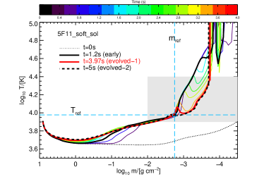
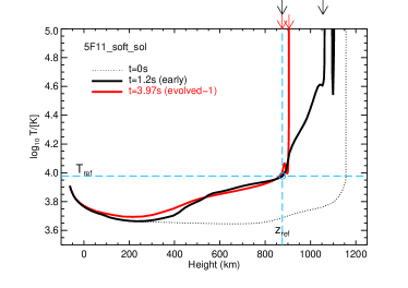
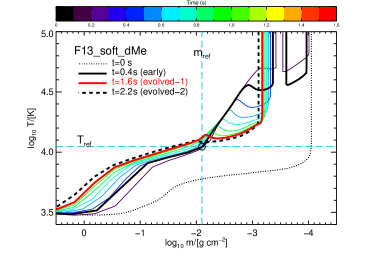
Figure 2: Temperature evolution as a function of column mass (top) and height (middle) in the 5F11$\_$soft$\_$sol model from $t=0-4$ s, shown at $\sim$0.4 s intervals and the evolved B time at $t=5$ s. The vertical dashed line indicates the value of log $m_{\rm{ref}}=-2.75$, and the horizontal dashed line indicates the temperature $T_{\rm{ref}}=9500$ K. A circle indicates the values of these parameters; the middle panel clearly demonstrates that these values indicate the temperature gradient change at the early time from $T\lesssim 10,000$ K to $T\gtrsim 10,000$ K. The arrows in the middle panel illustrate that the CC cools (from increased radiative losses) as it is compressed from a several hundred km region (between the black arrows) at the early time into a narrow 30 km region (between the red arrows) at the evolved-1 time. (Bottom) The temperature evolution of the F13$\_$soft$\_$dMe model for a dMe flare shown from $t=0-1.6$ s at 0.2 s intervals and at 2.2 s. The evolved-1 atmosphere is indicated at $t=1.6$ s and the evolved-2 is indicated at $t=2.2$ s, when the maximum $\lambda=3500$ Å continuum optical depth is achieved in the CC (Kowalski et al., 2015). The gray shaded area in the top panel indicates the column mass and temperature ranges in Figure 3.

2.3 Predicting the CC Evolution from $T_{\rm{ref}}$ and $m_{\rm{ref}}$

Larger values of $m_{\rm{ref}}$ produce larger continuum optical depth and larger emergent continuum intensity in the flare atmosphere. The maximum density in the evolved CC in the F13$\_$soft$\_$dMe RADYN model is $n_{\rm{H}}=7\times 10^{15}$ cm^-3 whereas the maximum density in the evolved CC in the 5F11$\_$soft$\_$sol RADYN model is $5\times 10^{14}$ cm^-3. As a result, the NUV (at $\lambda=3500$ Å) continuum optical depth in the CC in the F13 model is large, $\tau_{3500\rm{AA}}(\rm{CC})\sim 5$, whereas the NUV continuum optical depth in the CC in the 5F11$\_$soft$\_$sol model is smaller, $\tau_{3500\rm{AA}}(\rm{CC})=0.1$. Scaling relationships from $m_{\rm{ref}}$ (given that $T_{\rm{ref}}$ always occurs at $T\approx 10,000$ K) would be invaluable for comparison to NUV and blue spectral observations of flares in order to constrain the optical depth and electron density (Section 3).

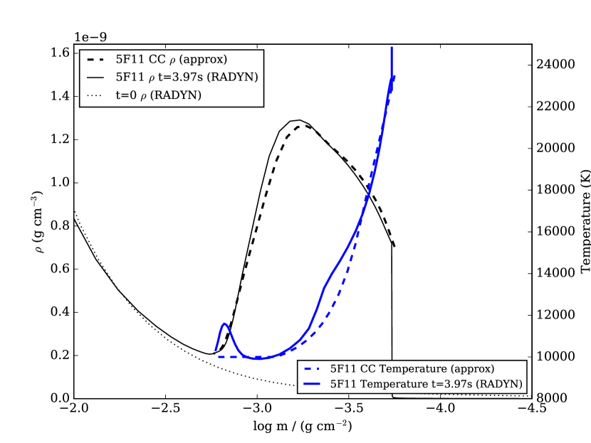
Figure 3: Enlarged view of the chromospheric condensation (CC) at the evolved-1 time ($t=3.97$ s) in the 5F11$\_$soft$\_$sol model at column mass corresponding to the gray shaded region in Figure 2. The density stratification at $t=0$ s in the solar atmosphere is shown as a dotted line for comparison. The approximate model of the CC density and temperature stratification at the evolved-1 time are shown as dashed lines. The parameters used for this are $x_{\rm{maxCC}}=30$ km, log $m_{\rm{ref}}=-2.75$, and $T_{\rm{ref}}=9500$ K, and $T_{\rm{minCC}}=10,000$ K (see text).

Using the RADYN calculation of the atmospheric response to a 5F11 beam flux density, we present a method to estimate the white-light continuum optical depth in evolved CCs and the emergent continuum intensity from the two flaring layers at the evolved times using only the parameters $T_{\rm{ref}}$ and log $m_{\rm{ref}}$ at early times. In this section we present the parameterization of the CC and the top of the stationary flare layers; in Section 2.3.1 we present the parameterized stratification of the stationary flare layers. Additional details are given in Appendix A.

To construct approximate evolved states of the CC, we take the following steps:

1. We obtain values of log $m_{\rm{ref}}$ and $T_{\rm{ref}}$ at early times in the RADYN simulations of Table 1. For very high (F13) beam flux density simulations, a time of $t=0.4$ s is adequate, whereas for lower beam flux density simulations such as for the 5F11$\_$soft$\_$sol  $t=1.2$ s is adequate. To obtain log $m_{\rm{ref}}$ and $T_{\rm{ref}}$ consistently for any set of models at their early times, we calculate the quantity $d$ log $T$/$d$ log $m$ and find the column mass where this quantity increases above $-0.3$ at the early times. At larger column mass than $m_{\rm{ref}}$, this derivative is near 0. At lower column mass, this derivative has much more negative values of $<-0.3$. The values of log $m_{\rm{ref}}$ and $T_{\rm{ref}}$ obtained in this way for each model are given in Table 2.

2. At the evolved-1 time of the 5F11$\_$soft$\_$sol  we obtain the temperature, velocity, mass density, and ionization fraction stratification for the regions of the atmosphere corresponding to temperatures $T\lesssim 25,000$ K and where $v_{z}<-5$ km s^-1. This region of the atmosphere corresponds to the cool, dense region of the CC. We define $z_{o}$ as the height corresponding to $T\approx 25,000$ K, where $z$ is the height variable from RADYN and $z=0$ occurs at $\tau_{5000\rm{AA}}=1$. We define the distance from the top of the CC to any lower height $z$ as $x=|z-z_{o}|$, where $x$ increases toward the pre-flare photosphere. For the 5F11$\_$soft$\_$sol model, we set $x_{\rm{maxCC}}=30$ km as the maximum physical depth range of the evolved CC as in the RADYN simulation.

   The density stratification of the evolved CCs in the F13$\_$hard$\_$dMe and F13$\_$soft$\_$dMe models are qualitatively similar to the evolved CC in the 5F11$\_$soft$\_$sol model, but they have a larger value of the maximum mass density ($\rho_{\rm{maxCC}}$) and a smaller physical depth range of $x_{\rm{maxCC}}\approx 18$ km. Compared to 30 km, a depth range of 18 km is very close to what the ratio of the surface gravities indicates for the physical depth range ($x_{\rm{maxCC}}$) of a compression in a dMe atmosphere with a higher gravity of log $g=4.75$. The CC in the solar atmosphere is more extended over height and exhibits a lower $\rho_{\rm{maxCC}}$ because of the lower surface gravity by a factor of two. In the solar CC, the lower mass density also results from a smaller amount of material that is compressed in the CC due to a smaller value of log $m_{\rm{ref}}$. The maximum density attained in a CC can also be affected by the velocity field such that much larger velocity gradients than in the 5F11$\_$soft$\_$sol model may produce a different density stratification in the CC; we discuss the role of this parameter for a higher electron beam flux density solar flare model in Section 3.2.

   Using the density stratification of the CC in the 5F11$\_$soft$\_$sol model at the evolved-1 time as a template, we create an approximate density stratification for any CC at the evolved-1 and evolved-2 times by applying values of log $m_{\rm{ref}}$, $T_{\rm{ref}}$, and log $g$ obtained at the early time. The advantage of this is that it predicts the evolved states directly from the early state without the expensive computations required to actually evolve the RADYN simulations. The CC density template ($\rho(x)_{\rm{norm}}$) is obtained by normalizing the density stratification of the CC at the evolved-1 time in the 5F11$\_$soft$\_$sol model by its maximum density ($\rho_{\rm{maxCC}}=1.3\times 10^{-9}$ g cm^-3). This density stratification is plotted in Figure 3.

   The CC density stratification template extends from the location where the speed of downflowing material falls below 5 km s^-1 (at the low temperature end, lower height end of the CC) to the location where the temperature exceeds $T=25,000$ K (at greater heights in the CC). The column mass at the low temperature end of the normalized density stratification ($\rho(x)_{\rm{norm}}$) is set to the value of $m_{\rm{ref}}$, and the height scale ($dx_{\rm{Sol}}$) of the template is adjusted according to the surface gravity. We solve the equation

   $$C\int_{x=0}^{x=30\rm{km}}\rho(x)_{\rm{norm}}\frac{10^{4.44}}{10^{\rm{log}g}}dx_{\rm{Sol}}=m_{\rm{ref}}$$ (2)

   for the constant $C$ to obtain a density stratification $C\rho(x)_{\rm{norm}}$ with units of g cm^-3 on a height scale $\frac{10^{4.44}}{10^{\rm{log}g}}dx_{\rm{Sol}}$ in units of cm, where $x_{\rm{maxCC}}=\int_{x=0}^{30\rm{km}}\frac{10^{4.44}}{10^{\rm{log}g}}dx_{\rm{Sol}}$. Before solving for $C$, we subtract 10% from $m_{\rm{ref}}$ in order to account for mass evaporated into the corona. The approximate evolved-1 atmosphere for the 5F11 compared to the RADYN calculation is shown in Figure 3. The approximate evolved-1 atmosphere for the F13$\_$hard$\_$dMe using the values of $m_{\rm{ref}}$ and $T_{\rm{ref}}$ in Table 2 and log $g=4.75$ ($x_{\rm{maxCC}}=15$ km) is shown in Figure 4 compared to the RADYN calculation. There is satisfactory agreement in the peak density and the general shape of the density stratification. At $x>2$ km, there is an exponential decay of the density from $\rho_{\rm{maxCC}}$ to the stationary flare layers in the RADYN calculation, and the approximate evolved-1 stratification exhibits a steeper decrease (smaller scale height) than in the RADYN calculation. This discrepancy is discussed further in Section 3.2.

   

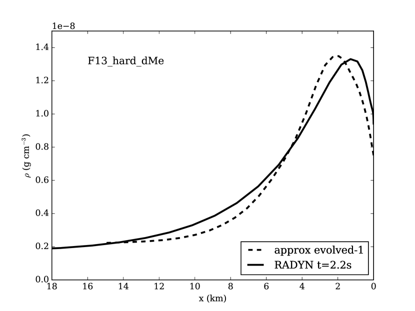
   Figure 4: The density stratification in the approximation at the evolved-1 time of the F13$\_$hard$\_$dMe model compared to the RADYN calculation at $t=2.2$ s. The top of the low-temperature ($T<25,000$ K) region of the CC is at $x=0$ km, and the bottom of the CC is at $x=x_{\rm{maxCC}}=15$ km. The density stratification was calculated from the density stratification template in Figure 3 using the value of log $m_{\rm{ref}}=-2.04$ in Equation 2.

3. Our template CC requires a temperature stratification, which we also obtain from the 5F11$\_$soft$\_$sol model. The minimum temperature ($T_{\rm{minCC}}$) in a CC at the evolved-1 time occurs at the height where $\rho\sim 3/4\times\rho_{\rm{maxCC}}$ at the higher column mass end of the CC. In Figure 3, $T_{\rm{minCC}}=10,000$ K occurs at log $m\sim-3.0$ and is near the value of $T_{\rm{ref}}=9500$ K: the CC has cooled to a temperature that is similar to the temperature at the top of the stationary flare layers. The value of $m_{\rm{ref}}$ at the evolved-1 time shifts to lower column mass (log$m\sim-3.3$ in the 5F11$\_$soft$\_$sol model) because most of the CC has cooled to $T\sim 10,000$ K and a significant fraction of hydrogen is not ionized in the evolved CC. The temperature stratification vs. column mass is qualitatively similar in the CCs among the 5F11$\_$soft$\_$sol and F13 models, but the the value of $T_{\rm{minCC}}$ is higher in the F13 models.

   We use the 5F11$\_$soft$\_$sol, F13$\_$soft$\_$dMe, and F13$\_$hard$\_$dMe models to prescribe simple adjustments to the temperature at the top of the stationary flare layers and the minimum temperature of the CC ($T_{\rm{minCC}}$)) because these temperatures are approximately equal at the evolved times. For the high beam flux density simulations, the temperatures in the stationary flare layers at $m>m_{\rm{ref}}$ increase by $\Delta T\sim 1500-2000$ K from the early to the evolved-1 times, and for the 5F11$\_$soft$\_$sol model the temperature at the bottom of the CC at the evolved-1 time is $\Delta T\sim 500$ K higher than the temperature indicated by $T_{\rm{ref}}$ at the early time. The amount by which the stationary flare layers increase in temperature through the simulation is sensitive to the hardness and flux of the electron beam distribution: harder beams and higher fluxes result in more heating and a higher (thermal) ionization fraction of hydrogen of the stationary flare layers (Kowalski et al., 2016). In the approximate evolved-1 model atmospheres, we simply take either $T_{\rm{minCC}}$(evolved-1)$=T_{\rm{ref}}\rm{(early)}+500$ K for the lower beam flux density (5F11) models or $T_{\rm{minCC}}$(evolved-1)$=T_{\rm{ref}}\rm{(early)}+1500$ K for the higher beam flux density (F13) models. The temperature at the top of the stationary flare layers at the evolved-1 times is set to $T_{\rm{minCC}}$.

   At the evolved-2 times in the RADYN simulations, the bottom of the CC at $x_{\rm{maxCC}}$ descends to $\sim 1.5$ times higher column mass than $m_{\rm{ref}}$. The maximum emergent continuum intensity occurs in the 5F11$\_$soft$\_$sol model, and the maximum continuum optical depth occurs in the F13$\_$soft$\_$dMe model. At the evolved-2 times, the values of $T_{\rm{minCC}}$ are $\sim 500$ K less than the values at the evolved-1 times because the CC has increased in density further and thus experiences more radiative cooling. We find that at the evolved-2 times in the RADYN simulations, the value of $m_{\rm{ref}}$ occurs where the density stratification of the CC decreases to $0.45$ times the maximum density in the CC. The approximate density stratification models at the evolved-2 times are calculated by evaluating Equation 2 with the upper limit of integration set to $x=10$ km, which is where $\rho(x)=0.45\rho_{\rm{maxCC}}$. At the evolved-2 times, the value of $x_{\rm{maxCC}}$ does not change, but the value of $m_{\rm{ref}}$ occurs at $\frac{1}{3}x_{\rm{maxCC}}$. We set $T_{\rm{minCC}}$(evolved-2)$=T_{\rm{ref}}\rm{(early)}$ for lower beam flux density (5F11) models and $T_{\rm{minCC}}$(evolved-2)$=T_{\rm{ref}}\rm{(early)}+1000$ K for higher beam flux density (F13) models. The temperature at the top of the stationary flare layers at the evolved-2 times is set to $T_{\rm{minCC}}$, as for the evolved-1 times.

   The details for establishing the temperature stratification at higher and lower heights than the height corresponding to $T_{\rm{minCC}}$ are presented in Appendix A. The approximate evolved-1 temperature stratification is shown in Figure 3 compared to the 5F11$\_$soft$\_$sol RADYN calculation.

4. To calculate the continuum optical depth within the approximate, evolved CC, we use LTE population densities of hydrogen and the H-minus ion. The evolved CCs become very dense in the RADYN simulations, and the hydrogen level populations are close to LTE values except at the upper $\sim 1$ km of the CC where the $n=1$ and $n=2$ populations depart significantly from their equilibrium values. From the mass density stratification of the CC, we convert to $n_{\rm{H,tot}}(x)$ using the gram per hydrogen value of 2.269$\times 10^{-24}$ for the solar abundance. From the temperature stratification of our approximate model CCs, we use the Saha-Boltzmann equation to solve for the hydrogen ionization fraction and the level populations as a function of height. We solve for the LTE electron density first by truncating the hydrogen atoms with $n_{\rm{max}}=10$. This approximate electron density is used to solve for the partition function and level population densities of hydrogen using the occupational probability formalism of Hummer & Mihalas (1988) with $n_{\rm{max}}=100$. Then, the we re-solve for the LTE electron density.

5. The equations for the hydrogen bound-free opacity, hydrogen free-free opacity, and H-minus bound-free opacity are used to calculate the continuum optical depth, at the base of the approximate, evolved CC, $\tau_{\lambda}(\rm{CC})$, using $x_{\rm{maxCC}}=15$ km for the dMe atmosphere and $x_{\rm{maxCC}}=30$ km for the solar atmosphere. Continuum opacities are corrected for stimulated emission.

   The results for several NUV and optical continuum wavelengths ($\lambda=2826,3500,4170,$ and 6010 Å) are shown in Table 2 compared to the optical depth calculated using the NLTE, NEI populations from RADYN and the continuum optical depth calculation method in Kowalski et al. (2017a). The NUV continuum wavelength $\lambda=2826$ Å corresponds to the NUV wavelengths observed by the Interface Region Imaging Spectrograph (IRIS; De Pontieu et al., 2014, and see section 3.5 here). The continuum wavelengths $\lambda=3500,4170,6010$ Å correspond to the central wavelengths of custom filters in the NUV, blue, and red, respectively, used to study dMe flares with the ULTRACAM instrument (Dhillon et al., 2007; Kowalski et al., 2016, and see section 3.4 here). The evolved-1 and the evolved-2 approximations are in excellent agreement with the continuum optical depth values at the bottom of the CCs at the respective times in the RADYN calculations. In the last two columns, we show that the maximum LTE electron density values in the approximate model CCs are generally consistent with the NLTE, NEI calculation from RADYN. We also show our predictions for the F13$\_$hard$\_$dMe model at the evolved-2 time, which is not calculated in RADYN simulation.

2.3.1 Approximating the Heating in the Stationary Flare Layers

To calculate the approximate emergent specific continuum intensity and emergent specific radiative flux density for comparison to observed flare spectra, we construct a simplified representation of the layers below the CC that are heated by the beam electrons with $E>>E_{\rm{c}}$. These stationary flare layers can contribute significantly to the emergent continuum radiation at $\lambda$ if the optical depth in the CC is $\tau_{\lambda}(\rm{CC})<1$; if $\tau_{\lambda}(\rm{CC})>1$ at some continuum wavelengths, the spectral shape of the emergent intensity will be modified from the spectral energy distribution that is expected from hydrogen recombination emissivity (Kowalski et al., 2015).

For the density stratification of the stationary flare layers, we either choose the solar or dMe pre-flare density stratification since material does not compress at these heights. We join the density stratification of the stationary flare layers to the CC to form a continuous density stratification in our approximate, evolved flare atmosphere. The details of the temperature stratification for the stationary flare layers is presented in Appendix A.2. In summary, the temperature decreases from $T_{\rm{minCC}}$ (at the top of the stationary flare layers) to $T_{\rm{minCC}}-3000$ K (at the bottom of the stationary flare layers) for hard ($\delta\sim 3$) beam models and to $T_{\rm{minCC}}-5000$ K (at the bottom of the stationary flare layers) for soft ($\delta\gtrsim 4$) beam models. The electron density in the stationary flare layers is determined under the LTE conditions from the given temperature stratification. We calculate the LTE populations of hydrogen and the H-minus ion and the continuum emissivity in the stationary flare layers as done in the CC (Section 2.3).

2.3.2 Emergent Continuum Spectra

The approximate evolved-1 temperature and electron density stratification for the F13$\_$hard$\_$dMe  model is shown in Figure 5 compared to the RADYN calculation of the electron density. Within the CC, the gas density is well-reproduced (see Figure 4). In the stationary flare layers, the maximum electron density and the electron density stratification is well-reproduced but the location of the maximum is offset towards greater heights. This discrepancy is a result of our simple way of appending the density stratification of the stationary flare layers to the evolved CC model.

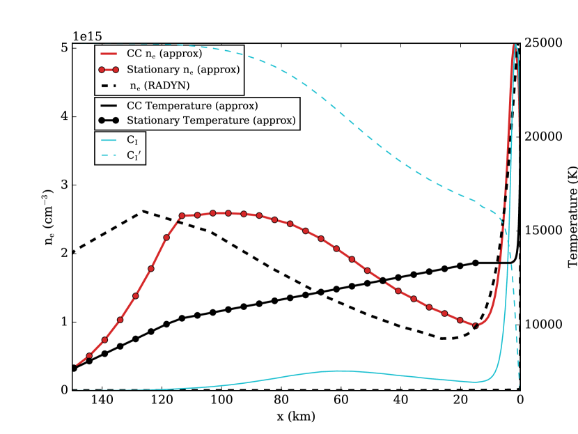
Figure 5: The RADYN calculation of the electron density at the evolved-1 time of the F13$\_$hard$\_$dMe model compared to our approximations. The temperature stratification from our approximations are also shown. The top of the CC corresponds to $x=0$ km and extends to $x=15$ km. The contribution function to the emergent blue continuum (4170 Å) intensity is shown as the solid light blue line normalized to the peak value, and the cumulative contribution function ($C_{I}^{\prime}$) is shown as the dashed light blue raning from 0 to 1 on the right axis. The approximate model for the evolved-1 time predicts the correct fraction (0.45) of the emergent blue continuum intensity originating from the stationary flare layers. In the RADYN simulation, the density decreases more than in the approximate model before the onset of the stationary flare layers, which results in the offset in the electron density to lower heights (larger values of $x$). However, the overall shape and magnitude of the electron density stratification is well reproduced with our approximations.

Multiplying the emissivity at all heights by $e^{-\tau_{\lambda}/\mu}/\mu$ and integrating over height gives the emergent continuum intensity from the simplified, evolved model atmospheres. We calculate the cumulative contribution function ($C_{I}^{\prime}$; Kowalski et al., 2017a) which allows us determine the fraction of emergent intensity originating from a height greater than $z$. The cumulative contribution function at $\lambda=4170$ Å is shown for our approximate model of the F13$\_$hard$\_$dMe simulation at the evolved-1 time in Figure 5. The physical depth range from $C_{I}^{\prime}=0.05$ to 0.95 for the emergent blue continuum intensity is $\Delta z=86$ km (vs. 95 km in RADYN), the fraction of emergent blue continuum intensity from the stationary flare layers is 0.46 (vs. 0.45 in RADYN), and the FWHM of the contribution function in the CC is 3.7 km (vs. 2.2 km in RADYN). Our approximate evolved-1 model atmosphere also satisfactorily reproduces the moderate ($\tau_{4170}(\rm{CC})\sim 0.5$) blue continuum optical depth in the CC (vs. $\tau_{4170}(\rm{CC})\sim 0.6$; Table 2), which is critical for producing the observed $T\sim 10,000$ K blackbody-like continua in the emergent radiative flux in these models (Kowalski et al., 2015, 2016).

We calculate the emergent specific radiative flux density, $F_{\lambda}$, using a Gaussian integral with the same five outgoing $\mu$ values employed in RADYN, in order to compare to unresolved stellar observations. The results for the Balmer jump ratio, $F_{\lambda=3500}/F_{\lambda=4170}$ (FcolorB), in the emergent radiative flux spectra compared to the RADYN calculations in Kowalski et al. (2016) are shown in Table 2. Large Balmer jump ratios of FcolorB$>8$ are produced in the 5F11$\_$soft$\_$sol model and the evolved approximations, whereas small Balmer jump ratios of FcolorB$\lesssim 2$ are produced in the F13 RADYN calculations and the evolved atmosphere approximations. Furthermore, a smaller Balmer jump ratio is produced in the F13$\_$hard$\_$dMe  evolved-1 model than in either of the evolved approximations of the F13$\_$soft$\_$dMe  as in the RADYN calculations. A lower Balmer jump ratio in the emergent radiative flux spectrum in the evolved-1 approximation of the F13$\_$hard$\_$dMe  is due to the combination of the lower optical depth in the CC ($\tau_{\rm{4170}}(\rm{CC})\sim 0.6$ in the F13$\_$hard$\_$dMe  vs. $\tau_{\rm{4170}}(\rm{CC})\sim 0.8$ in the F13$\_$soft$\_$dMe), and the higher temperatures (and thus with larger ambient electron density and larger continuum emissivity) in the stationary flare layers in comparison to the evolved-2 time in the F13$\_$soft$\_$dMe (see Kowalski et al., 2016). The evolved-2 time of the F13$\_$hard$\_$dMe  has a smaller Balmer jump ratio than the evolved-1 time due to a very large change in optical depth from $\tau\sim 3$ to $\sim 7$ in the CC at $\lambda=3500$ Å, resulting in a net decrease in emergent intensity from the atmosphere. At the evolved-2 time, nearly $\sim 25$% of the emergent blue $\lambda=4170$ Å  continuum intensity originates from the heated stationary flare layers with very high electron density ($\sim 3\times 10^{15}$ cm^-3) even though the optical depth in the CC, $\tau_{4170}(\rm{CC})$, is greater than 1.

Table 2: Approximate Model Atmospheres: Continuum optical depth and emergent intensity

RADYN Model (time)	log $m_{\rm{ref}}$/g cm-2	$T_{\rm{ref}}$ [K] ($T_{\rm{minCC}}$ [K])	$\tau_{\rm{3500\AA}}(\rm{CC})$		$\tau_{\rm{4170\AA}}(\rm{CC})$		$\tau_{\rm{2826\AA}}(\rm{CC})$		$\tau_{\rm{6010\AA}}(\rm{CC})$		$F_{3500{\rm{\AA}}}/F_{4170{\rm{\AA}}}$		max $n_{e}/10^{14}$ cm-3
–	–	–	approx	RAD	approx	RAD	approx	RAD	approx	RAD	approx	RAD	approx	RAD
5F11$\_$soft$\_$sol evolved-1 (3.97 s)	-2.75 ($t=1.2$ s)	9500 (10,000)	0.10	0.10	0.01	0.01	0.05	0.06	0.03	0.03	9.1	8.2	4.9	5.3
5F11$\_$soft$\_$sol evolved-2 (5 s)	-2.75 ($t=1.2$ s)	9500 (9500)	0.15	0.18	0.02	0.02	0.09	0.10	0.04	0.04	8.6	8.0	7.2	6.7
F13$\_$soft$\_$dMe evolved-1 (1.6 s)	-2.10 ($t=0.4$ s)	11,100 (12,600)	2.4	2.0	0.39	0.4	1.3	1.1	1.0	0.9	2.3	2.6	40	50
F13$\_$soft$\_$dMe evolved-2 (2.2 s)	-2.10 ($t=0.4$ s)	11,100 (12,100)	4.9	5.4	0.75	0.8	2.7	3.0	2.0	2.2	1.94	2.1	54	62
F13$\_$hard$\_$dMe evolved-1 (2.2 s)	-2.04 ($t=0.4$ s)	11,800 (13,300)	2.89	3.4	0.52	0.6	1.6	1.9	1.4	1.5	1.78	1.8	51	51
F13$\_$hard$\_$dMe evolved-2 (–)	-2.04 ($t=0.4$ s)	11,800 (12,800)	6.6	–	1.1	–	3.7	–	2.9	–	1.7	–	67	–

Note. — The optical depth values at several continuum windows ($\lambda=3500,4170,2826,6010$ Å) are calculated at the bottom of the CC where the downflowing speed decreases below 5 km s^-1. A value of $\mu=0.95$ was used for the optical depth calculations in the approximate model (“approx”’) to compare to a $\mu$ value in the RADYN (“RAD”) calculation. The values of FcolorB for the F13 models calculated with RADYN were obtained from Kowalski et al. (2016). For the evolved-1 approximations, we compare to the RADYN simulations at $t=3.97$ s in the 5F11$\_$soft$\_$sol RADYN model, $t=1.6$ s in the F13$\_$soft$\_$dMe RADYN model, and $t=2.2$ s in the F13$\_$hard$\_$dMe  RADYN model. The evolved-2 approximation of the F13$\_$soft$\_$dMe model is compared to $t=2.2$ s in the RADYN calculation. To obtain $T_{\rm{min,CC}}$ for the lower beam flux density evolved atmospheres, we add 500 K to $T_{\rm{ref}}$ at evolved-1 times and no increase to $T_{\rm{ref}}$ at evolved-2 times. To obtain $T_{\rm{minCC}}$ for the high beam flux density evolved atmospheres, we add 1500 K to $T_{\rm{ref}}$ for the evolved-1 approximations and 1000 K to $T_{\rm{ref}}$ for the evolved-2 approximations. The values of $F_{3500{\rm{\AA}}}/F_{4170{\rm{\AA}}}$ indicate the Balmer jump ratios, FcolorB, of the emergent radiative flux density spectrum in units of erg cm^-2 s^-1 Å^-1.

3 Discussion and Application

Our prescription for parameterizing RHD flare models is an alternative modeling approach to traditional phenomenological/semi-empirical, static flare modeling that varies atmospheric parameters through a large possible range (Machado et al., 1980; Cram & Woods, 1982; Avrett et al., 1986; Machado et al., 1989; Mauas et al., 1990; Christian et al., 2003; Schmidt et al., 2012; Fuhrmeister et al., 2010; Rubio da Costa & Kleint, 2017; Kuridze et al., 2017) or static synthetic, beam-heated models (e.g., Ricchiazzi & Canfield, 1983; Hawley & Fisher, 1994). Many of these models are currently widely used (e.g., Heinzel & Avrett, 2012; Trottet et al., 2015; Kleint et al., 2016; Simões et al., 2017). When velocity or the position of the flare transition region is modified in phenomenological models, the gas density must also change and is not correctly given by hydrostatic equilibrium. In our approximate models, we employ density stratifications that self-consistently result from pressure and velocity gradients in the atmosphere. The evolved-1 and evolved-2 approximate model atmospheres can be used to explore large grids of model predictions for the NUV and optical continuum radiation for values of $m_{\rm{ref}}$, $T_{\rm{ref}}$, and log $g$; an interesting parameter space can then be investigated with RHD simulations for NLTE predictions of the emission line profiles with accurate treatments of broadening, non-equilibrium ionization/excitation, and backwarming of the photosphere/upper photosphere.

There are several assumptions made in our prescription that limit the accuracy of the continuum predictions in the approximate evolved-1 and evolved-2 atmospheres.

• First, one must assume a temperature stratification of the stationary flare layers to obtain the emergent intensity. We assume either $\Delta T=-3000$ K (for hard beams) or $\Delta T=-5000$ K (for soft beams) over the height range of the stationary flare layers. To approximate the temperature evolution of the stationary flare layers from the early to evolved times, we assume either no increase occurs or values of $\Delta T=+500$ K, 1000 K, or 1500 K occurs as in the RADYN simulations. The precise values depend on the flux density, hardness, and evolution of the electron beam energy deposition.

  For variable beam parameters over short times, such as the inferred soft-hard-soft power-law index variation (Grigis & Benz, 2004), the values of $m_{\rm{ref}}$ and $T_{\rm{ref}}$ may change significantly and RADYN simulations are required.

• Second, our prescription assumes LTE, which is satisfactory for the optical and NUV continuum wavelength predictions for CCs that become sufficiently dense. At the evolved-1 time of the 5F11$\_$soft$\_$sol model, the assumption of LTE results in a small error in the $n=2$ opacity in the uppermost 1 km of the CC. Using the snapshot calculated at $t=3.97$ s by the RH code (Uitenbroek, 2001) and the contribution function analysis from Kowalski et al. (2017a), we find that approximately 10% of the emergent NUV continuum intensity originates from the top of the CC where the NLTE population density of $n=2$ departs by more than 1.7 from LTE; the $n\geq 3$ populations exist at their LTE values.

• Third, our approximate model atmospheres do not include a parameterization of heating in the upper photosphere, such as from radiative backwarming due to Balmer and Paschen continuum photons (Allred et al., 2006). Low to moderate heating ($\Delta T\lesssim 1000$ K) of the upper solar photosphere by backwarming does not produce significant continuum radiation at NUV wavelengths (Kleint et al., 2016) but it does affect the Balmer jump ratio due to the increase of H^- emissivity from the upper photosphere at red optical wavelengths in the 5F11$\_$soft$\_$sol RADYN model (Appendix A of Kowalski et al., 2017a). The upper photospheric heating is not included in our approximations, which results in larger Balmer jump ratios than with backwarming included in the RADYN calculations (see Table 2). In the F13$\_$hard$\_$dMe and F13$\_$soft$\_$dMe models, radiation from upper photospheric heating does not contribute to the emergent radiation at any wavelength because the stationary flare layers and the CC are optically thick at NUV and optical continuum wavelengths.

• Fourth, approximations for atmospheres with a surface gravity that differs from log $g=4.75$ and log $g=4.44$ do not include the modifications to the density stratification in the CC from large deviations of the velocity field compared to the 5F11 template stratification (see Section 3.2), and they do not include modifications of the density stratification of the stationary flare layers (see Section 3.3.1). More templates for a range of heating scenarios and surface gravities can be easily included in future work if needed.

• Finally, flares consist of heating and cooling loops; multithread modeling with complete RHD calculations (Warren, 2006; Rubio da Costa et al., 2016; Osten et al., 2016) are required for a direct comparison to spatially unresolved observations. The Balmer jump ratios from multithread modeling are larger than the extreme values attained at the evolved-1 or evolved-2 times. In future work, an approximate decay phase parameterization can be developed for a course superposition of an early-time (from RADYN), an evolved time (an evolved-1 or evolved-2 approximation), and a decay-time (approximation) as a multithread model (e.g. following Kowalski et al., 2017b) to compare directly to observations.

The agreement between the Balmer jump ratios in the RADYN simulation and the approximate evolved models (Table 2) justifies these assumptions and approximations. The prescription for estimating the optical depth and emergent continuum intensity in a flare atmosphere consisting of a cooled CC and heated stationary flare layers at pre-flare chromospheric heights has important applications for interpreting and understanding the NUV and optical continuum radiation in solar and stellar flares. In this section, we present several applications of our approximate model atmospheres: constraining flare heating scenarios that produce intermediate Balmer jump ratios as observed in some impulsive phase dMe flare spectra (Section 3.1), understanding the role of surface gravity on the CC density evolution (Section 3.2, 3.3.1), determining the threshold for hot blackbody radiation in the impulsive phase of dMe flares (Section 3.3), understanding the interflare variation and relationship among peak flare colors (Section 3.4), and constraining models of solar flares with IRIS data of the NUV ($\lambda\sim 2830$ Å) flare continuum intensity (Section 3.5).

3.1 Application to dMe Flares: Intermediate Balmer Jump Ratios

The Balmer jump ratio values from the approximate evolved models (Table 2) can be used to distinguish flare heating scenarios with NUV and optical continuum radiation formed from material at $T\sim 10,000$ K over low (e.g., as in the 5F11 model) and high (e.g., as in the F13 models) continuum optical depth. As an application to dMe flare spectra, we derive the value of $m_{\rm{ref}}$ to be achieved at an early time in an RHD flare simulation to produce an intermediate Balmer jump ratio between FcolorB $\lesssim 2$ (as in the F13 models) and FcolorB $\gtrsim 8$ (as in the 5F11 model). Values in the range of FcolorB $=3-4$ have been observed at the peak times of several flares in EV Lac (Kowalski et al., 2013) and YZ CMi (Kowalski et al., 2016). The hybrid-type (HF) and gradual-type flare (GF) events classified in Kowalski et al. (2013) and Kowalski et al. (2016) always exhibit these intermediate values of the Balmer jump ratio in the impulsive phase; some impulsive-type flare (IF) events also exhibit these values at peak times (Kowalski et al., 2016), while the gradual decay phases of all types of flare events can be characterized by intermediate Balmer jump ratios $\gtrsim 2.75$ (Kowalski et al., 2013, 2016). Thus, the intermediate Balmer jump ratio values are an important observed phenomenon to reproduce with RHD models.

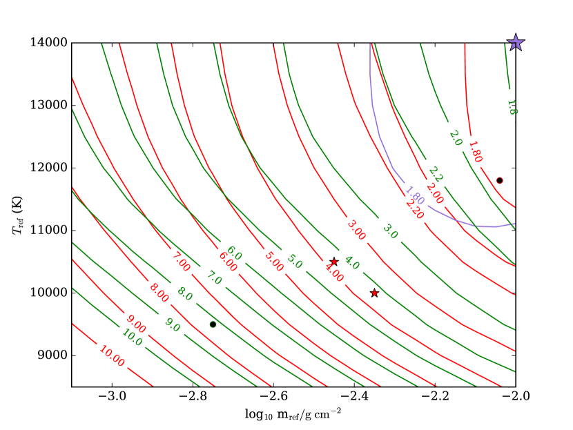
Figure 6: Contours of the Balmer jump ratio, $F_{3500}/F_{4170}$, denoted as FcolorB in Kowalski et al. (2016). Red contours correspond to the dMe model approximations ($x_{\rm{maxCC}}=15$ km), and green contours correspond to the solar model approximations ($x_{\rm{maxCC}}=30$ km). We use the evolved-1 approximation with $T_{\rm{minCC}}=T_{\rm{ref}}+1500$ K; the heating in the stationary flare layers is approximated for a hard electron beam distribution for all calculations (see text). Red stars indicate example dMe flare evolved-1 atmospheres that produce an intermediate Balmer jump ratio of FcolorB$=3.6-3.8$. The black circles indicate the Balmer jump ratios from the approximate models at the evolved-1 times for the 5F11$\_$soft$\_$sol model (Figure 3) and the F13$\_$hard$\_$dMe model (Figure 5). The purple contour shows the range of parameters that produce a Balmer jump ratio of FcolorB $=1.8$ in the evolved-2 approximation for the dMe surface gravity. For the dMe gravity, the lowest Balmer jump ratio in this parameter space for the evolved-2 approximation is 1.6 which is indicated by the purple star; the lowest Balmer jump ratio in the parameter space for the evolved-1 approximation is 1.7.

In Figure 6, we show contours of the Balmer jump ratio, FcolorB, for a range of $T_{\rm{ref}}$ and log $m_{\rm{ref}}$, calculated in intervals of 500 K and 0.05, respectively, with our approximate models at the evolved-1 times. The Balmer jump ratio has been calculated for the dMe surface gravity in red contours. For large values of $m_{\rm{ref}}$, the Balmer jump ratio decreases for increasing $T_{\rm{ref}}$ at constant $m_{\rm{ref}}$ and for increasing $m_{\rm{ref}}$ at constant $T_{\rm{ref}}$.

The evolved-1 times represent a conservative estimate to the minimum Balmer jump ratio attained in an RHD model. The Balmer jump ratio becomes lower at the evolved-2 time because the CC attains a higher column mass by a factor of $\sim 1.5$; the minimum Balmer jump ratio depends on the poorly constrained duration of high beam flux heating in a flare loop. We show a purple contour in Figure 6 for the value of FcolorB $=1.8$ to illustrate the difference between the evolved-1 and evolved-2 times. In the upper right corner of Figure 6, the lowest Balmer jump ratio is 1.7 in the evolved-1 approximation and 1.6 in the evolved-2 approximation.

Red star symbols on this figure show that an intermediate Balmer jump ratio of FcolorB$=3.6-3.8$ at the peak of a dMe flare can be produced by an atmosphere with $T_{\rm{ref}}=10^{4}$ K and log $m_{\rm{ref}}=-2.35$ or with $T_{\rm{ref}}=10,500$ K and $m_{\rm{ref}}=-2.45$. At these values, the optical depth (at $\mu=0.95$) within the CC at $\lambda=4170$ Å is $\sim 0.1$ and at $\lambda=3500$ Å the optical depth is between $0.6-0.9$: because $\tau_{3500}$ in the CC is near one, a significant amount of outgoing Balmer continuum radiation from the stationary flare layers is attenuated, and the Balmer jump ratio in an emergent spectrum is smaller than the Balmer jump ratio in an emergent spectrum formed at $T\sim 10^{4}$ K over low continuum optical depth. The maximum value of the electron density that results in a CC with log $m_{\rm{ref}}=-2.35$ is $n_{e}\sim 2\times 10^{15}$ cm^-3. Thus, we expect broad hydrogen lines from CCs that produce the intermediate Balmer jump ratio, but NLTE modeling with an accurate broadening treatment is required for detailed line shapes (Kowalski et al., 2017b). Results from the approximate evolved-1 atmospheres will be used to compare to new RHD models with high low-energy cutoff values in a future work on flares with intermediate Balmer jump ratios observed in the dM4e star GJ 1243 (Kowalski et al. 2018A, in prep).

3.2 Application to Superflares in Rapidly Rotating dG Stars

The approximate model atmospheres can be used to understand how the emergent continuum spectral properties vary in flares occurring in stars over a range of surface gravity values. The heating in the lower atmosphere in superflares ($E_{\rm{white-light}}\approx 10^{35}-10^{36}$ erg) observed by Kepler in rapidly rotating, young dG stars (Maehara et al., 2012) is not yet understood. Compared to the largest flares in the present day Sun, do these superflares result from larger average energy flux densities in electron beams and/or do they exhibit larger flare areas? In this section, we explore the Balmer jump ratio expected from lower surface gravity solar-type stars, though such constraints are currently not readily available for solar flares or dG superflares.

Contours of the Balmer jump ratio calculated with the value of $x_{\rm{maxCC}}=30$ km (for solar surface gravity) are shown as the green contours in Figure 6. All other parameters are kept the same in these evolved-1 calculations compared to the dMe (red) contours with stationary flare layer heating estimated for a hard electron beam distribution. For similar values of $T_{\rm{ref}}$ and log $m_{\rm{ref}}$, the solar atmosphere produces larger values of the Balmer jump ratio FcolorB. This difference occurs due to the different surface gravitational acceleration, log $g$, by a factor of two. For the same electron beam flux density and beam energy distribution in a dG and dMe star flare, a similar column mass is heated by the beam (Allred et al., 2006), and we expect this to produce a similar value of $m_{\rm{ref}}$ among atmospheres of different gravity. The factor of two larger gravity in a dMe star and the same value of log $m_{\rm{ref}}$ means that this column mass of material is compressed into a factor of $\frac{10^{4.75}}{10^{4.44}}=2$ smaller physical depth range. The value of $m_{\rm{ref}}$ is an area in $\rho(z)$ vs. $z$, which results in a larger value of $\rho_{\rm{maxCC}}$, continuum optical depth, and maximum electron density in a CC.

For large beam flux densities near F13, however, the relationship between gravity and Balmer jump ratio becomes more complicated than implied by the scaling in Equation 2. We run a RADYN flare simulation of the solar atmospheric response to a very high beam flux density, F13, $\delta=3$, $E_{c}=37$ (hereafter, F13$\_$hard$\_$sol), for direct comparison to the F13$\_$hard$\_$dMe and F13$\_$soft$\_$dMe models. The energy deposition lasts for 4.5 s, at which point the coronal temperature exceeds 100 MK, which is the upper limit to the atomic data currently in RADYN. The physical depth range of the CC in the F13$\_$hard$\_$sol simulation is $x_{\rm{maxCC}}\sim 30$ km, confirming that this parameter is independent of the beam flux density and is inversely proportional to the surface gravitational acceleration. At $t=0.4$ s, we calculate that log $m_{\rm{ref}}=-1.96$ and $T_{\rm{ref}}=11,650$ K using the algorithm in Section 2; note that these values are similar to the values that result from flare heating in the F13$\_$hard$\_$dMe RADYN model (Table 2). The approximate evolved-2 atmosphere prescriptions predict that the maximum electron density in the CC is $4.3\times 10^{15}$ cm^-3, the optical depth at $\lambda=4170$ Å at the bottom of the CC is 0.9 and the value of FcolorB is 1.7. In the F13$\_$hard$\_$sol RADYN calculation, the maximum electron density in the CC is much larger $\sim 7\times 10^{15}$ cm^-3 compared to this prediction. We inspect the density stratification of the F13$\_$hard$\_$sol model compared to the template density stratification obtained from the 5F11$\_$soft$\_$sol at the evolved-1 time (Figure 3). There is a significant difference in the density stratification compared to the 5F11$\_$soft$\_$sol density template stratification. In the F13$\_$hard$\_$sol model, much larger downflow speeds of 200 km s^-1 occur, compared to $\sim 50-60$ km s^-1 in the 5F11$\_$soft$\_$sol and $90-100$ kms^-1 in the F13$\_$hard$\_$dMe and F13$\_$soft$\_$dMe models.

From Equation 2, the larger gravity of the dMe atmosphere results in more atmospheric compression over height; a similar value of $m_{\rm{ref}}$ is expected to produce a factor of $\sim 2$ lower maximum density in a solar model atmosphere for the same beam flux density of F13. However, the RADYN F13$\_$hard$\_$dMe and F13$\_$hard$\_$sol simulations have roughly the same maximum density ($\rho_{\rm{maxCC}}$) in the CCs. The analytic calculations from Fisher (1989) show that the pre-flare chromospheric density just below the flare transition region is inversely related to the maximum downflow speed. The F13$\_$hard$\_$sol and F13$\_$hard$\_$dMe models exhibit a similar value of $m_{\rm{ref}}$ (to within 20%), but the initial uncompressed density just below the flare transition region is smaller in the solar atmosphere (also by a factor of two) which results in $\sim$two times larger maximum downflow speeds ($\sim 200$ km s^-1) in the solar CC. The product of the maximum downflow speed ($v$) and preflare gas density ($\rho$) below the flare transition region gives a similar initial mass flux density (in units of $g$ cm^-2 s^-1) in the two F13 models. Using the template gas density stratification from the 5F11$\_$soft$\_$sol model implicitly assumes that the mass flux density (which determines the amount of gas compression and thus $\rho_{\rm{maxCC}}$) is controlled by the ratio of preflare gas density values below the flare transition region and is not influenced strongly by much larger or smaller initial downflow speeds.

The solar contours in Figure 6 therefore underestimate the values of the actual Balmer jump ratios of the emergent spectra. The RADYN simulation shows that the Balmer jump ratio at the evolved-1 time (2.2 s) is 1.7 compared to 1.9 in Figure 6; at the evolved-2 time (2.8 s), the Balmer jump ratio attains a value as low as 1.5 in RADYN, compared to the evolved-2 approximation of 1.7. Furthermore, the Balmer jump ratio in the F13$\_$hard$\_$sol model is lower than our predicted Balmer jump ratio at the evolved-2 time of the F13$\_$hard$\_$dMe model (Table 2). By adjusting the 5F11$\_$soft$\_$sol density stratification template using the difference in downflow speeds between the F13$\_$hard$\_$sol and 5F11$\_$soft$\_$sol models, we predict an electron density of $6.6\times 10^{15}$ cm^-3 and a larger blue continuum optical depth at the bottom of the CC ($\tau_{4170}(\rm{CC})\sim 1.1$) for log $m_{\rm{ref}}=-1.96$. These are closer to the values in the F13$\_$hard$\_$sol RADYN simulation ($7\times 10^{15}$ cm^-3 and 1.2, respectively). The template from the 5F11$\_$soft$\_$sol model is accurate for predictions of the maximum electron density in the CC for a limited range of downflow speeds to within a factor of the 5F11$\_$soft$\_$sol maximum downflow speeds.

Simultaneous X-ray and optical spectra of dG superflares would determine if high flux electron beam flux densities are generated in young solar-like stars. Notably, large energy flux densities between F12 and F13 have been inferred in bright solar flare kernels (Neidig et al., 1993; Krucker et al., 2011; Sharykin et al., 2017), and we may expect values of the Balmer jump ratio as low as FcolorB $\lesssim 2$ in spatially resolved, solar flare spectra as well as in spectra of dG superflares.

3.3 Application to dMe Flares: Hot Blackody-like Radiation

In the impulsive phase of some dMe flares, an energetically important observed spectral property is a color temperature of $T\sim 9000-14,000$ K in the blue and red optical wavelength range (Hawley & Pettersen, 1991; Zhilyaev et al., 2007; Fuhrmeister et al., 2008; Kowalski et al., 2013). The emergent flux spectra with a color temperature of $T\sim 9000-14,000$ K also exhibit small Balmer jump ratios (FcolorB$<$2; cf Figure 12 of Kowalski et al., 2016). We calculate the FcolorR continuum flux ratio, $F_{4170}/F_{6010}$, which is a proxy of the blue-to-red optical color temperature (Kowalski et al., 2016) for our approximate model atmospheres. Contours are shown in Figure 7 for the evolved-1 atmosphere approximations with stationary flare layers heated by a hard beam ($\delta\sim 3$). We define “hot” color temperatures as $T_{\rm{FcolorR}}\geq 8500$ K, corresponding to FcolorR $=1.7$ and the thick red contour. This thick contour is the threshold that we establish for producing hot blackbody-like radiation for a high electron beam flux with a hard power-law distribution. We do not address here the property of some flares exhibiting blue optical continua ($\lambda=4000-4800$ Å) with a larger color temperature (by $\Delta T\sim 2000$ K) than indicated by $T_{\rm{FcolorR}}$ (Kowalski et al., 2013, 2016); our approximate models here generally produce a blue color temperature lower than $T_{\rm{FcolorR}}$ by several hundred K.

The F13$\_$hard$\_$dMe and F13$\_$soft$\_$dMe models reproduce hot color temperatures at their evolved-1 and evolved-2 times and possibly explain this interesting spectral phenomenon (Kowalski et al., 2013, 2016). The location of the evolved-1 time of the F13$\_$hard$\_$dMe model is shown in Figure 7 as a black circle. Detailed modeling of optical spectra with the RH code shows that extremely broad Balmer lines result from the high charge density ($n_{e}\sim 5\times 10^{15}$ cm^-3) in the CC (Kowalski et al., 2017b). Also shown in Figure 7 are contours of the maximum (LTE) electron density achieved in the evolved-1 approximations. We thus expect very high electron densities in the CCs for the range of FcolorR values that are consistent with the hot color temperature observations. A large beam flux density is expected to produce a strong return current electric field and beam instabilities (Holman, 2012; Li et al., 2014), which were not included in any of the RADYN simulations or approximations in this work. Also, the coronal magnetic field energy that is converted to kinetic energy during reconnection must be $B\sim$1.5 kG (Kowalski et al., 2015). These issues place constraints on the highest beam flux density that is possible in the atmospheres of stars. The values of $m_{\rm{ref}}$ and $T_{\rm{ref}}$ from any future RHD model with lower beam flux density than F13 can be placed on Figure 7 (or a similar figure for soft $\delta\gtrsim 4$ electron beams; not shown) and compared to the thick red contour to determine if the model is expected to produce hot blackbody continuum radiation at $\lambda>4000$ Å.

3.3.1 Implications for High Gravity dMe Flare Models

The RADYN simulations of dMe flares that are used to produce the contours in Figures 6 - 7 have log $g=4.75$. Using the fundamental parameter relationships in Mann et al. (2015) and the magnitude and distance information from Reid & Hawley (2005), we calculate that the surface gravity values for AD Leo (dM3e), YZ CMi (dM4.5e), and Proxima Centauri (dM5.5e) to be log $g=4.83$, log $g=4.9$, and log $g=5.26$, respectively. We show purple contours in Figure 7 for the approximate FcolorR values from evolved-1 atmospheres with a CC having a physical depth range of $x_{\rm{maxCC}}=8$ km, which is estimated as the physical depth range of a CC in an atmosphere with log $g=5$. We adjust the physical depth of the stationary flare layers according to the surface gravity (Appendix A.2) but no change is made to the density stratification in the stationary flare layers compared to the log $g=4.75$ hydrostatic equilibrium stratification. The purple contours in Figure 7 indicate that lower electron beam flux density values may result in similar valus of $m_{\rm{ref}}$ but larger CC densities and continuum optical depths in high gravity M dwarfs. Changing the surface gravity would also affect the maximum downflow speed for the same nonthermal beam density (Section 3.2), and accurate approximations for higher surface gravity may require a CC density stratification template from a new hydrodynamic simulation. We suggest that RADYN calculations explore higher surface gravity values of log $g>4.75$.

A large sample of flux ratio measurements (e.g., with ULTRACAM; Dhillon et al., 2007; Kowalski et al., 2016) of flares in stars spanning stars of the subtypes dM0e-dM7e with similar values of log $L_{\rm{H}\alpha}$ / $L_{\rm{bol}}$ would test whether surface gravity affects the appearance of optical color temperatures of $T_{\rm{FcolorR}}\geq$ 8500 K and small Balmer jump ratios of FcolorB$<$2 in the observed spectra. Curiously, the Great Flare of AD Leo, which has a log $g=4.83$ that is close to the RADYN model atmosphere (as chosen initially), exhibits a very small Balmer jump ratio of $1.4-1.8$ and a hot optical flare blackbody (Hawley & Pettersen, 1991; Hawley & Fisher, 1992; Kowalski et al., 2013). Thus a larger surface gravity with a significantly lower beam flux density (and thus a smaller value of $m_{\rm{ref}}$ for a comparably large value of FcolorR $\gtrsim 2$) cannot account for these flare properties in all active M dwarf stars.

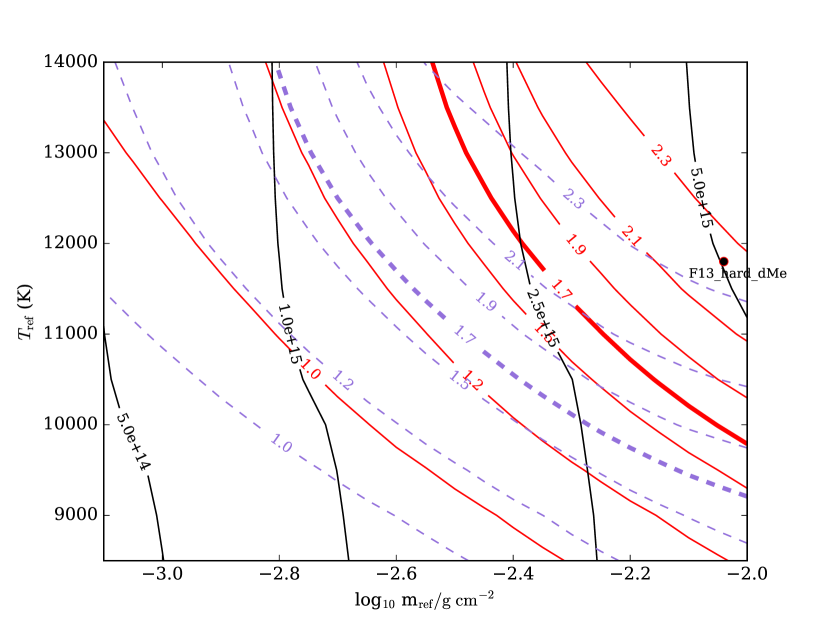
Figure 7: Contours of the blue ($\lambda=4170$ Å) continuum flux divided by the red ($\lambda=6010$ Å) continuum flux, referred to as FcolorR in Kowalski et al. (2016), for the evolved-1 approximations (with hard beam heating). We set $T_{\rm{min,CC}}=T_{\rm{ref}}+1500$ K for all calculations. Red contours correspond to the dMe model approximations ($x_{\rm{max,CC}}=15$ km). The black circles indicates the ratios from the approximate model of the F13$\_$hard$\_$dMe RADYN simulation at the evolved-1 time. The color temperatures, $T_{\rm{FcolorR}}$, corresponding to these contours are $T_{\rm{FcolorR}}=(5800,6500,7600,8500,9300,10400,11600)$ K for FcolorR $=(1.0,1.2,1.5,1.7,1.9,2.1,2.3)$, respectively. Also shown are contours for the maximum electron density produced in the evolved-1 models of the CC. The maximum electron density is always greater than $2\times 10^{15}$ cm^-3 for the atmospheres that have $m_{\rm{ref}}$ and $T_{\rm{ref}}$ that also produce hot ($T_{\rm{FcolorR}}\geq 8500$ K; thick red contour) color temperature that characterizes the blue-to-red optical continuum. The dashed purple contours indicate the values of FcolorR for evolved-1 approximations in a dMe atmosphere with $x_{\rm{maxCC}}=8$ km to mimic the compression in an atmosphere with log $g=5$. No adjustment for the density stratification of the stationary flare layers was made compared to the log $g=4.75$ red contours. The thick red contour is our determination for the threshold for forming a hot blackbody flux spectrum at $\lambda>4000$ Å for hard electron beams.

3.4 Application to dMe Flares: The Interflare Variation of Peak Continuum Flux Ratios

In Figure 8, we show the relationship between FcolorR and FcolorB predicted from our approximate evolved-1 atmospheres by varying log $m_{\rm{ref}}$ from -3.1 to -1.7 and keeping $T_{\rm{ref}}=11,000$ K ($T_{\rm{minCC}}=12,500$ K) constant. The flare peak data from Kowalski et al. (2016) shows that the range of impulsive phase continuum flux ratios may result from variations of $m_{\rm{ref}}$ from flare to flare. The $t=2.2$ s continuum flux ratio values for the F13$\_$hard$\_$dMe and F13$\_$soft$\_$dMe are shown also as a light gray and black star, respectively. Kowalski et al. (2016) proposed that the differences in the hardness of the electron beam between these two models may suggest that interflare peak variation is due to beam hardness variations. In our approximations, varying the value of $m_{\rm{ref}}$ represents changing the electron beam hardness and flux density.

The approximate model relationship falls significantly below the values of FcolorB for five of the flares with ULTRACAM data in Figure 8. Larger observed values of FcolorB than in the evolved-1 time approximations indicate that relatively more Balmer continuum radiation is produced in the impulsive phase than is accounted for by variations of $m_{\rm{ref}}$. This “missing” Balmer continuum radiation in the approximate model representation may result from flare loops that are heated in the early rise phase and gradually decay through the impulsive phase (e.g., see Warren, 2006). A multithread analysis of the F13$\_$soft$\_$dMe and F13$\_$hard$\_$dMe RADYN models reveals that superposing all snapshots of these models increase FcolorB but also decrease FcolorR (cf Table 1 of Kowalski et al., 2017b). We show these multithread model values in Figure 8 as black and light gray circles. The multithread models do not account for the large Balmer jump ratios at high values of FcolorR, nor do they account for the intermediate Balmer jump ratios of FcolorB $>3$ (Section 3.1).

In Figure 8, we have extended the range of log $m_{\rm{ref}}$ to $-1.7$ in order to reproduce some of the largest observed values of FcolorR. Such a large value of log $m_{\rm{ref}}$ suggests an electron beam flux density $>$ F13 and thus a very strong return current electric field. Neither this extreme value of log $m_{\rm{ref}}=-1.7$ and $T_{\rm{ref}}=11,000$ K nor the largest values in Figure 6 (for log $m_{\rm{ref}}=-2$ and $T_{\rm{ref}}=14,000$ K) produce the smallest values of FcolorB$\sim 1.4-1.5$ observed at the main peaks of other dMe flares (Hawley & Pettersen, 1991) and in some energetic secondary flares (Kowalski et al., 2013).

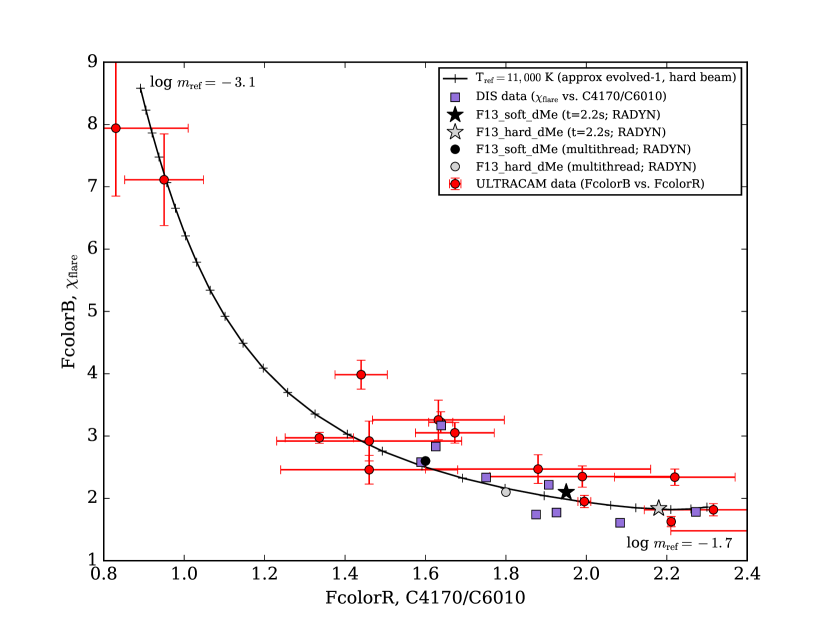
Figure 8: The relationship for FcolorB vs. FcolorR with $T_{\rm{ref}}=11,000$ K in the approximate evolved-1 models. The value of log $m_{\rm{ref}}$ is varied from -3.1 to -1.7. The photometry data from Figure 12 of Kowalski et al. (2016) are shown as red circles (from ULTRACAM), and the continuum flux ratios from the Apache Point Observatory’s ARC 3.5-m/DIS spectra (from Kowalski et al., 2013) are shown as purple squares (where $\chi_{\rm{flare}}$ is similar to FcolorB and C4170/C6010 is similar to FcolorR). The observed relationship is generally reproduced by varying log $m_{\rm{ref}}$. However, the largest values of FcolorR are only produced by an extreme value of log $m_{\rm{ref}}=-1.7$, and some flares exhibit a significant offset towards larger values of the Balmer jump ratio. Note that there are several flares at very large values of FcolorR $>2.4$ that are not shown here; these secondary flare events may be explained by a very high low-energy cutoff electron beam heating function (Kowalski et al., 2017b). The values for the RADYN F13$\_$hard$\_$dMe (at the evolved-1 time) and F13$\_$soft$\_$dMe (at the evolved-2 time) are shown as gray and black stars, respectively; the average burst (multithread) model for each are shown as gray and black circles respectively.

3.5 Application to dG Flares: NUV Continuum Intensity in IRIS Spectra

High spectral resolution and high time resolution observations of the brightest kernels in the hard X-ray impulsive phase of solar flares exhibit a redshifted component in the singly ionized chromospheric lines (Graham & Cauzzi, 2015) and in H$\alpha$ (Ichimoto & Kurokawa, 1984) which is conclusive evidence for the formation of dense CCs. Bright NUV continuum intensity is also predicted from dense CCs (Kowalski et al., 2017a), and high spatial resolution spectra of bright kernels in solar flares are now readily available from IRIS to compare to high beam flux density RHD models.

The NUV spectra from IRIS include a continuum region at $\lambda=2825.6-2826.9$ Å (hereafter, “IRIS NUV” or “C2826” as referred to in Kowalski et al. (2017a)) outside of major and minor emission lines, where the Balmer-continuum enhancement was first detected by Heinzel & Kleint (2014). The bright emergent continuum intensity in the 5F11$\_$soft$\_$sol RADYN model attains a brightness (and becomes brighter) than the observed values of C2826 in the 2014-March-29 X1 solar flare. We calculate the emergent NUV continuum intensity from our evolved-1 and evolved-2 model atmospheres using the values of $T_{\rm{ref}}$ and log $m_{\rm{ref}}$ in the RADYN calculation. The emergent excess intensity at $\lambda=2826$ Å in the 5F11$\_$soft$\_$sol RADYN model at $t=3.97-5$ s is $5-5.5\times 10^{6}$ erg cm^-2 s^-1 Å^-1 sr^-1(Kowalski et al., 2017a) and is consistent with the range of emergent intensity predicted by our approximate evolved-1 ($I_{\lambda=2826,\mu=0.77}=5.0\times 10^{6}$ erg cm^-2 s^-1 Å^-1 sr^-1) and evolved-2 ($I_{\lambda=2826,\mu=0.77}=6.5\times 10^{6}$ erg cm^-2 s^-1 Å^-1 sr^-1) atmospheres. In this case, the evolved-1 and evolved-2 atmospheres provide lower and upper limits, respectively, to compare to observational constraints from IRIS. The approximate values of $\tau_{2826}$ at the bottom of the CC are shown in Table 2; there is satisfactory agreement between our approximations and the NLTE, NEI calculations with RADYN.

A lower beam flux density of F11 was used in Kowalski et al. (2017a) for comparison to the 5F11 model (see also Kuridze et al., 2015, 2016, for detailed analyses of the F11 model). The F11 results in faint NUV continuum intensity that is not consistent with the observations of the two brightest flaring footpoints at their brightest observed times in the 2014-Mar-29 flare, thus favoring a higher beam flux density for these kernels. The low-energy cutoff that was used was $E_{c}=25$ keV as inferred from hard X-ray fitting of RHESSI data. As well known, this is an upper limit to the low energy cutoff that can be inferred from the data due to a bright thermal X-ray spectrum at lower energies. We use our approximate, evolved model atmospheres to determine if a lower beam flux density of F11 and a lower low-energy cutoff ($E<<25$ keV) reproduces the observed NUV continuum intensity in the two brightest flare kernels in the 2014-Mar-29 X1 flare. We use the RADYN code to simulate the atmospheric response to an F11 beam flux density with $E_{c}=15$ keV and $\delta=3.6$, which are also consistent with the hard X-ray observations (Battaglia et al., 2015). This value of $\delta$ is harder than the F11 model with $\delta=4.2$ presented in Kowalski et al. (2017a). Following the Fe II LTE line analysis in Kowalski et al. (2017a), we find that the harder F11 model with the lower low-energy cutoff produces two Fe II 2814.45 emission line components that are consistent with the formation of a CC and stationary flare layers. The F11 with $E_{c}=25$ keV in Kowalski et al. (2017a) does not produce a red shifted emission component in Fe II. In this new RADYN model, we obtain the values of log $m_{\rm{ref}}=-3.08$ and $T_{\rm{ref}}=8900$ K at the early time of $t=1.2$ s. The approximate emergent intensity at the evolved-1 time (with the soft beam heating approximation in the stationary flare layers) matches the value of $10^{6}$ erg cm^-2 s^-1 Å^-1 sr^-1 in the RADYN simulation. The approximate model at the evolved-2 time (with the hard beam heating approximation in the stationary flare layers) predicts an emergent continuum NUV intensity of $1.4\times 10^{6}$ erg cm^-2 s^-1 Å^-1 sr^-1  which is nearly a factor of two below the observed excess C2826 values of $\gtrsim 2.2\times 10^{6}$ erg cm^-2 s^-1 Å^-1 sr^-1 in the two brightest footpoints BFP1 and BFP2 in the 2014-March-29 X1 flare. Therefore, a F11 flux density cannot reproduce the brightest NUV continuum intensity observed in this flare; this heating scenario is an insufficient model for understanding the atmospheric processes in the brightest continuum-emitting kernels. However, representative values of C2826 for this flare are $<1.5\times 10^{6}$ erg cm^-2 s^-1 Å^-1 sr^-1 (Kleint et al., 2016) and these fainter flaring pixels may be explained by lower heating rates. Our new F11 RADYN flare model and a new 2F11 RADYN flare model (also with $E_{c}=15$ and $\delta=3.6$) will be discussed in more detail in comparison to observations of the hydrogen line broadening in a future paper (Kowalski et al. 2018B, in prep).

4 Summary and Conclusions

We have developed a prescription to predict the approximate values of the NUV and optical continuum optical depth, the emergent continuum intensity, the continuum flux ratios, and the maximum electron density attained in flare atmospheres exhibiting an evolved, cooling compression above stationary heated layers with $T\approx 10^{4}$ K. The prescription depends on specifying only two parameters besides the gravity of the star: $T_{\rm{ref}}$ and log $m_{\rm{ref}}$, which can be readily obtained at early times in radiative-hydrodynamic simulations such as with the RADYN code. The approximate, evolved atmospheres provide interesting electron beam parameter space selection ($\delta$, $E_{c}$, flux density) for computationally intensive RADYN and Flarix (Heinzel et al., 2016) simulations of the non-LTE, non-equilibrium ionization/excitation hydrogen Balmer line and singly ionized chromospheric line profiles. Our analysis of $m_{\rm{ref}}$ and $T_{\rm{ref}}$ can also be applied to future 3D flare models that can resolve the large pressure gradients that drive these chromospheric condensations. 3D NLTE RHD models will be more computationally expensive than the current 1D NLTE RHD simulations, and a selective range of electron beam parameters will be necessary. Given a CC density stratification template, our prescription and analysis can be applied to any flare heating scenario that produces two flare layers at pre-flare chromospheric heights.

The approximate models of the evolved states of a CC have been used to determine the values of $T_{\rm{ref}}$ and log $m_{\rm{ref}}$ that produce blue optical continuum radiation ($\lambda=4170$ Å) formed in two, $T\sim 10^{4}$ K flare layers with a large optical depth ($\tau_{4170}=0.4-1.2$), an intermediate optical depth ($\tau_{4170}\sim 0.15$), and a low optical depth ($\tau_{4170}<<0.1$). Very high beam energy deposition rates as in the F13 models produce $m_{\rm{ref}}\sim 0.01$ g cm^-2 and a large optical depth ($\tau_{4170}=0.4-1.2$) in the $T\sim 10,000$ K material in the CC, which results in a larger optical depth and smaller physical depth range at NUV and red wavelengths due to the wavelength dependence of hydrogen b-f opacity. A large optical depth produces an emergent continuum spectrum with a color temperature of $T\sim 10,000$ K and a small Balmer jump ratio as observed in the impulsive phase of dMe flares (Kowalski et al., 2013). We have determined a critical threshold contour of $T_{\rm{ref}}$ and log $m_{\rm{ref}}$ (Figure 7) for producing the hot blackbody radiation. This threshold can be compared to values obtained from lower beam flux density simulations than F13, which results in a very strong return current electric field (to be included in the energy loss in the electron beam in a future work) and requires strong magnetic fields in the corona. Our prescription predicts that high ambient electron densities of $n_{e}>2\times 10^{15}$ cm^-3 in the CC are produced for all significantly large values greater than log $m_{\rm{ref}}=-2.4$.

Our approximations are accurate enough to distinguish between flare atmospheres that result in a large Balmer jump ratio (low optical depth at all continuum wavelengths) and a smaller Balmer jump ratio (intermediate or high optical depth at all continuum wavelengths). Observations of the peak phases of dMe flares exhibit a range of properties, and variation of $m_{\rm{ref}}$ in our approximate model atmospheres cover most of the observed relationship between the Balmer jump ratio and blue-to-red optical color temperature (Figure 8). Some dMe flares exhibit intermediate Balmer jump ratios at the peak of the impulsive phase. Our prescription predicts that electron beam heating resulting in log $m_{\rm{ref}}\sim-2.35$ to $-2.45$ at early times would produce an intermediate Balmer jump ratio in the evolved states of the atmosphere. For these evolved model atmospheres, $\tau_{3500}\sim 1$ and $\tau_{4170}\sim 0.15$ at the bottom of the CCs. We expect that lower beam energy flux densities than F13 can produce such emergent flux spectra with intermediate Balmer jump ratios, which are also observed in the gradual decay phase of dMe flares.

The CC density and emergent continuum properties depend on stellar surface gravity in a complex way. Generally, larger surface gravity stars produce denser CCs and larger continuum optical depth values. For F13 electron beam flux densities, our approximations predict that smaller Balmer jump ratios and hotter blue-to-red optical continua are produced in the models of dMe flares compared to flares in the Sun and rapidly rotating dG stars. However, the lower gas density initially below the flare transition region in lower surface gravity stars causes a larger downflow velocity in the CC (Fisher, 1989). A much larger downflow velocity ($v$) and a smaller preflare gas density ($\rho$) produces a comparable mass flux density (in units of $g$ cm^-2 s^-1) and thus a similar value of $\rho_{\rm{maxCC}}$ and continuum optical depth compared to the response of a higher gravity star to an F13 beam flux density. We discussed a new solar F13 flare model, which may explain the radiation from superflares in rapidly rotating dG stars; the density stratification template from this RADYN model exhibits a much different velocity field than the CCs in the solar 5F11 and dMe F13 models and can be used to make more refined predictions for the emergent spectral properties at large values of $m_{\rm{ref}}$ (e.g., in Figures 6 - 7) when observational constraints of the continuum flux ratios during flares exist for these stars.

Using the density stratification of the CC in the solar 5F11 model from Kowalski et al. (2017a) as a template for our approximate model atmospheres, one can predict the emergent $\lambda=2826$ Å NUV continuum intensity in IRIS data of solar flares, for which Fe II and Mg II line profiles suggest that chromospheric condensations are produced in the impulsive phase. A relatively low beam energy flux density (F11) with values of $E_{c}$ and $\delta$ that are within the hard X-ray observational constraints but outside the limited parameter space explored previously in the literature (e.g., Kowalski et al., 2017a), does not reproduce the two brightest observed excess IRIS NUV continuum intensity values in the 2014-March-29 X1 solar flare. We have confirmed this with a new RADYN calculation. Therefore, a higher flux density is required to reach the largest observed $\lambda=2826$ Å NUV continuum brightness in this X-class flare, and our approximate calculations can be used to guide RADYN modeling of other flares observed with IRIS.

In Appendix B, we present an extension of our model prescriptions: calculations of the emergent continuum flux from CCs with $T>>10,000$ K, which was suggested to explain the optical continuum flux ratios in Kowalski (2012). In future work, we will also extend our approximate prescriptions to RADYN atmospheres heated by electron beams with a high low-energy cutoff $\gtrsim 100$ keV. Lower beam flux densities with a high low-energy cutoff in the electron distribution can reproduce a small Balmer jump ratio, a hot red-to-blue optical continuum, and narrow Balmer lines (e.g., the $E_{c}=150$ keV 5F12 model in Appendix A of Kowalski et al., 2017b).

A Python GUI is freely available for the approximate evolved-1 and evolved-2 model atmosphere calculations upon request to the first author. Appendix B demonstrates how broad wavelength continuum flux spectra can be constructed from our algorithm to fill in continuum regions of the flare spectrum without constraints from observations. If the Balmer jump ratio of a flare is constrained, we suggest that our approximate model atmospheres could be useful for modeling the effects of ultraviolet flare radiation on exoplanet atmospheres (e.g. Segura et al., 2010; Ranjan et al., 2017). Approximations for wavelength regimes that are not possible to observe in solar flares will also be useful for addressing flare energy budget problems (Fletcher et al., 2007; Milligan et al., 2014; Kleint et al., 2016).

Appendix A: The Algorithm for the Temperature Stratification of our Approximate Flare Atmospheres

In this Appendix, we present the details of our algorithm for constructing a temperature stratification for the approximate model atmospheres in the CC and in the stationary flare layers.

A.1. Temperature within the CC

At the column masses in the CC that are less than where $T_{\rm{minCC}}$ occurs, we approximate the temperature from $T_{\rm{minCC}}$ to $T=17,000$ K as an exponential rise vs. log $m$. From $T=17,000$ K to $25,000$ K (at $x=0$), a linear rise with log $m$ is used. The column mass corresponding to $T=25,000$ K is chosen as log $m_{\rm{ref}}-1.0$, since $\sim$10% of the column mass is at higher temperatures in the flare transition region and corona. The temperature stratification at low heights in the CC is assumed to be constant and equal to $T_{\rm{minCC}}$. In Figure 3, there is a local temperature maximum at the highest column mass of the CC in the RADYN calculation due to viscous and compressive heating contributions (Kowalski et al., 2015); ignoring this feature in our approximations does not make a difference in our results.

A.2. Temperature within the stationary flare layers

At the evolved times in the RADYN calculations, the temperature at the top of the stationary flare layers is set to the value of $T_{\rm{minCC}}$, which is determined from $T_{\rm{ref}}$ with the simple adjustments described in Section 2.3. For harder electron beam ($\delta\sim 3$) simulations, the electron density in the stationary flare layers is higher than in softer ($\delta\gtrsim 4$) beams. We find that a linear temperature decrease of 3000 K adequately reproduces the ambient electron density in the F13$\_$hard$\_$dMe simulation and a linear temperature decrease of 5000 K adequately reproduces the ambient electron density in the F13$\_$soft$\_$dMe and 5F11$\_$soft$\_$sol simulations, which have softer distributions of nonthermal electrons at the energies that heat the stationary flare layers. The gravitational acceleration determines the height range below the CC over which these temperature drops occur. Due to the differences in log $g$, the total physical depth range of the stationary flare layers is $\Delta z=150$ km for the dMe and $\Delta z=300$ km for the solar atmosphere.

In summary, the temperature stratification of the stationary flare layers heated by electron beams are determined as follows:

• Evolved-A, lower beam flux densities (5F11): $T=T_{\rm{ref}}+500$ K at the top of the stationary flare layers and bottom of the CC ($x=x_{\rm{maxCC}}$); the temperature stratification linearly decreases by $\Delta T=3000$ K for hard electron beams ($\Delta T=5000$ K for soft electron beams) extending to $x=x_{\rm{maxCC}}+100$ km below the CC (for the dMe) and 200 km below the CC (for the solar atmosphere) .

• Evolved-2, lower beam flux densities (5F11): $T=T_{\rm{ref}}$ at the top of the stationary flare layers and bottom of the CC ($x=x_{\rm{maxCC}}$); the temperature stratification linearly decreases by $\Delta T=3000$ K for hard electron beams ($\Delta T=5000$ K for soft electron beams) extending to $x=x_{\rm{maxCC}}+100$ km below the CC (for the dMe) and 200 km below the CC (for the solar atmosphere).

• Evolved-A, high beam flux densities (F13): $T=T_{\rm{ref}}+1500$ K at the top of the stationary flare layers and bottom of the CC ($x=x_{\rm{maxCC}}$); the temperature stratification linearly decreases by $\Delta T=3000$ K for hard electron beams ($\Delta T=5000$ K for soft electron beams) extending to $x=x_{\rm{maxCC}}+100$ km below the CC (for the dMe) and 200 km below the CC (for the solar atmosphere).

• Evolved-2, high beam flux densities (F13): $T=T_{\rm{ref}}+1000$ K at the top of the stationary flare layers and bottom of the CC ($x=x_{\rm{maxCC}}$); the temperature stratification linearly decreases by $\Delta T=3000$ K for hard electron beams ($\Delta T=5000$ K for soft electron beams) extending to $x=x_{\rm{maxCC}}+100$ km below the CC (for the dMe) and 200 km below the CC (for the solar atmosphere).

For all approximate model atmospheres, the bottom of the stationary flare layers extends to $x=x_{\rm{maxCC}}+150$ km for the dMe ($x=x_{\rm{maxCC}}+300$ km for the solar atmosphere). We adjust the physical depth range linearly for other values of the surface gravity, but no change is made to the density in the stationary flare layers compared to the solar and dMe pre-flare density stratification. The temperature at the bottom of the stationary flare layers is set to $T=6500$ K. At these lowermost flare layers in our approximate evolved models, the optical depth is either too large for any emission to escape or the emissivity is small compared to the emissivity in the higher layers. Therefore, our results are not sensitive to the details at such low temperature.

Appendix B: Superhot $T\sim 10^{5}$ K CCs in dMe Flares?

A “superhot” plasma with $T\sim 170,000$ K produces the $\lambda>3500$ Å continuum properties that are generally consistent with some spectra in the impulsive phase of a large YZ CMi flare with a red continuum exhibiting a cooler color temperature (cf Figure 7.6 of Kowalski, 2012, and Kowalski et al. (2013)). We calculate the emergent spectrum from a “superhot CC” (where superhot refers to $T\sim 10^{5}$ K or greater) using our evolved atmosphere approximations with $T_{\rm{minCC}}=170,000$ K and log $m_{\rm{ref}}=-2.3$. The flux spectrum is shown in Figure 9 from the far-ultraviolet through the optical, which exhibits a value of FcolorB $=1.5$ and FcolorR $=1.8$. The evolved-1 density in this CC is $n_{e}>10^{15}$ cm^-3 and results in a low continuum optical depth $\tau_{\lambda}\lesssim 0.01$. The dominant continuum emissivity is free-free (thermal bremsstrahlung) emission. The contribution to the emergent intensity from the stationary flare layers is not included in this calculation (the emissivity from these layers is set to 0) in order to isolate the spectral properties of the superhot layers. If stationary flare layers at $T\sim 10^{4}$ K are included in the calculation, then the emergent spectrum exhibits a larger Balmer jump ratio due to the hydrogen recombination radiation from the stationary flare layers with a comparable electron density of $n_{e}\sim 10^{15}$ cm^-3. The superhot CC model exhibits a physical depth range that is $10^{4}$ times larger than the path length (of several meters) of material at $T=10^{5}-2\times 10^{5}$ K in the high flux density (5F11-F13) electron beam RADYN models. The physical depth range of the $T\sim 10^{5}$ K thermal bremsstrahlung would have to be much larger than currently predicted in the RADYN models to contribute significantly to the emergent radiation if there are also stationary flare layers at lower temperature, as concluded for solar flare spectra early on (Hiei, 1982).

In the $T=170,000$ K slab model in Kowalski (2012), the Gaunt factors were assumed to be equal to 1, which results in a Balmer jump ratio and FcolorR values that appear to be consistent with the observational comparison. Including the wavelength dependent Gaunt factors in the calculations here changes the spectral shape considerably. We use the free-free Gaunt factors from (Menzel & Pekeris, 1935) (as used in the RADYN code) and bound-free Gaunt factors from (Seaton, 1960) (as used in the RH code) and find that a very large value of log $m_{\rm{ref}}=-1.7$ and lower $T_{\rm{ref}}\sim 75,000$ K give more reasonable values of the Balmer jump ratio ($\sim 1.8$) and FcolorR values ($\sim 2$) compared to the observations in Kowalski (2012). This superhot CC spectrum is shown in Figure 9 scaled by a factor of 0.1. Such a large value of $m_{\rm{ref}}$ produces $n_{e}\sim 10^{16}$ cm^-3 in the CC.

In Figure 9 we also show the spectrum from the approximate F13$\_$hard$\_$dMe model at the evolved-2 time (with parameters given in the last row of Table 2), which produces heating to $T\sim 10,000$ K at densities of $n>10^{15}$ cm^-3. Compared to the superhot approximation $T_{\rm{ref}}\sim 75,000$ K, the F13$\_$hard$\_$dMe approximation exhibits a similar color temperature at $\lambda>4000$ Å and Balmer jump ratio but an opposite continuum slope at $\lambda<2500$ Å. In the very early phases of the F13$\_$hard$\_$dMe RADYN model ($t\sim 0.1$ s), the temperature of the CC over a significant path length ($\Delta z\sim 15$ km) is at a temperature of $T\sim 75,000$ K but this material has a much lower column mass than log $m_{\rm{ref}}=-1.7$. Most of the emergent optical continuum radiation originates from lower temperature at this very early time in the RADYN simulation, and the CC quickly cools below 75,000 K in a short time ($\Delta t\lesssim 0.05$ s).

Too few spectral observations of the continuum at $\lambda<3500$ Å exist during dMe flares to definitely rule out the existence of a $T>50,000$ K CC in dMe flares. Course broadband photometry of a moderate-sized flare in AD Leo indicates that the spectral energy distribution decreases from NUV to FUV wavelengths (Hawley et al., 2003). An IUE/FUV spectrum exists for the first 900 s of the impulsive phase of the Great Flare in AD Leo (Hawley & Pettersen, 1991), showing a rather flat FUV continuum distribution. This flare exhibits a very low Balmer jump ratio, and Hawley & Fisher (1992) demonstrates that the broadband photometry distribution rules out a $T\sim 1$ MK free-free continuum in favor of a $T\sim 9500$ K blackbody distribution. NUV spectra at $\lambda<3500$ Å were not obtained during the impulsive phase of this flare. Clearly, more NUV data at $\lambda<3500$ Å are critical to completely rule out the rising spectral characteristics of a superhot CC spectrum in some flares. If we add the F13$\_$hard$\_$dMe approximate evolved-2 spectrum and the superhot ($T=75,000$ K) CC spectrum in Figure 9 we obtain a nearly flat FUV continuum distribution as observed in the Great Flare impulsive phase (cf Figure 6 of Hawley & Pettersen, 1991). The superhot CC spectrum was multiplied by a filling factor of 0.1 relative to the F13 approximate spectrum. One could speculate that a very short persistence of flare kernels with dense, $T=50,000-100,000$ K plasma and F13 beam-heated kernels (with an order of magnitude larger area) may also help explain the faster time FUV time-evolution compared to the NUV (Hawley et al., 2003) and the very high observed FUV/NUV flux ratios in GALEX data (Robinson et al., 2005; Welsh et al., 2006) of the impulsive phase of dMe flares.

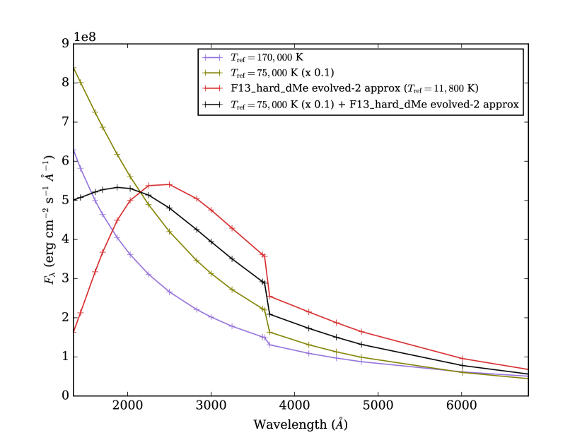
Figure 9: Flare spectra at $\lambda=1300$Å to 6800Å from approximate evolved atmosphere calculations that are all generally consistent with impulsive phase observations of dMe flares at $\lambda>3500$ Å. Thermal bremsstrahlung radiation from a dense, superhot CC with $T=170,000$ K (log $m_{\rm{ref}}=-2.3$) is shown as the purple curve, a superhot CC with $T=75,000$ K (log $m_{\rm{ref}}=-1.7$) multiplied by 0.1 is shown as the olive curve, the approximate evolved-2 F13$\_$hard$\_$dMe is shown as the red curve, and a superposition of the $T=75,000$ K (log $m_{\rm{ref}}=-1.7$) CC model multiplied by 0.1 and the approximate evolved-2 F13$\_$hard$\_$dMe model is shown as the black curve. For the superhot models, the emissivity from the stationary flare layers was not included in the calculation of the emergent radiative flux. All models exhibit small Balmer jump ratios, a color temperature at blue and red optical wavelengths of $T_{\rm{FcolorR}}>8500$ K, and a rising spectrum from 3600 Å to 2600 Å. The red spectrum peaks at $\lambda\sim 2500$ Å and turns over into the FUV. The superposed spectrum exhibits a relatively flat distribution in the FUV and a peak near $\lambda\sim 2000$ Å. Spectral data at $\lambda<2500$ Å would be able to constrain the role of very hot, very dense chromospheric condensations in the impulsive phase of dMe flares. The light purple model exhibits a smaller Balmer jump ratio and FcolorR value compared to the 170,000 K slab model in Kowalski (2012) due to including the values of the Gaunt factors in these new predictions.

References

- Abbett & Hawley (1999) Abbett, W. P., & Hawley, S. L. 1999, ApJ, 521, 906
- Allred et al. (2005) Allred, J. C., Hawley, S. L., Abbett, W. P., & Carlsson, M. 2005, ApJ, 630, 573
- Allred et al. (2006) —. 2006, ApJ, 644, 484
- Allred et al. (2015) Allred, J. C., Kowalski, A. F., & Carlsson, M. 2015, ApJ, 809, 104
- Avrett et al. (1986) Avrett, E. H., Machado, M. E., & Kurucz, R. L. 1986, in The lower atmosphere of solar flares, p. 216 - 281, ed. D. F. Neidig, 216–281
- Battaglia et al. (2015) Battaglia, M., Kleint, L., Krucker, S., & Graham, D. 2015, ApJ, 813, 113
- Canfield & Gayley (1987) Canfield, R. C., & Gayley, K. G. 1987, ApJ, 322, 999
- Carlsson & Stein (1992) Carlsson, M., & Stein, R. F. 1992, ApJ, 397, L59
- Carlsson & Stein (1994) Carlsson, M., & Stein, R. F. 1994, in Chromospheric Dynamics, ed. M. Carlsson, 47
- Carlsson & Stein (1995) —. 1995, ApJ, 440, L29
- Carlsson & Stein (1997) —. 1997, ApJ, 481, 500
- Carlsson & Stein (2002) —. 2002, ApJ, 572, 626
- Christian et al. (2003) Christian, D. J., Mathioudakis, M., Jevremović, D., et al. 2003, ApJ, 593, L105
- Cram & Woods (1982) Cram, L. E., & Woods, D. T. 1982, ApJ, 257, 269
- De Pontieu et al. (2014) De Pontieu, B., Title, A. M., Lemen, J. R., et al. 2014, Sol. Phys., 289, 2733
- Dhillon et al. (2007) Dhillon, V. S., Marsh, T. R., Stevenson, M. J., et al. 2007, MNRAS, 378, 825
- Dorfi & Drury (1987) Dorfi, E. A., & Drury, L. O. 1987, Journal of Computational Physics, 69, 175
- Dulk (1985) Dulk, G. A. 1985, ARA&A, 23, 169
- Emslie (1978) Emslie, A. G. 1978, ApJ, 224, 241
- Emslie (1981) —. 1981, ApJ, 245, 711
- Emslie & Nagai (1985) Emslie, A. G., & Nagai, F. 1985, ApJ, 288, 779
- Fisher (1989) Fisher, G. H. 1989, ApJ, 346, 1019
- Fisher et al. (1985a) Fisher, G. H., Canfield, R. C., & McClymont, A. N. 1985a, ApJ, 289, 434
- Fisher et al. (1985b) —. 1985b, ApJ, 289, 414
- Fletcher et al. (2007) Fletcher, L., Hannah, I. G., Hudson, H. S., & Metcalf, T. R. 2007, ApJ, 656, 1187
- Fuhrmeister et al. (2008) Fuhrmeister, B., Liefke, C., Schmitt, J. H. M. M., & Reiners, A. 2008, A&A, 487, 293
- Fuhrmeister et al. (2010) Fuhrmeister, B., Schmitt, J. H. M. M., & Hauschildt, P. H. 2010, A&A, 511, A83
- Gan et al. (1992) Gan, W. Q., Rieger, E., Zhang, H. Q., & Fang, C. 1992, ApJ, 397, 694
- Graham & Cauzzi (2015) Graham, D. R., & Cauzzi, G. 2015, ApJ, 807, L22
- Grigis & Benz (2004) Grigis, P. C., & Benz, A. O. 2004, A&A, 426, 1093
- Hawley & Fisher (1992) Hawley, S. L., & Fisher, G. H. 1992, ApJS, 78, 565
- Hawley & Fisher (1994) —. 1994, ApJ, 426, 387
- Hawley & Pettersen (1991) Hawley, S. L., & Pettersen, B. R. 1991, ApJ, 378, 725
- Hawley et al. (2003) Hawley, S. L., Allred, J. C., Johns-Krull, C. M., et al. 2003, ApJ, 597, 535
- Heinzel & Avrett (2012) Heinzel, P., & Avrett, E. H. 2012, Sol. Phys., 277, 31
- Heinzel et al. (2016) Heinzel, P., Kašparová, J., Varady, M., Karlický, M., & Moravec, Z. 2016, in IAU Symposium, Vol. 320, Solar and Stellar Flares and their Effects on Planets, ed. A. G. Kosovichev, S. L. Hawley, & P. Heinzel, 233–238
- Heinzel & Kleint (2014) Heinzel, P., & Kleint, L. 2014, ApJ, 794, L23
- Hiei (1982) Hiei, E. 1982, Sol. Phys., 80, 113
- Holman (2012) Holman, G. D. 2012, ApJ, 745, 52
- Hummer & Mihalas (1988) Hummer, D. G., & Mihalas, D. 1988, ApJ, 331, 794
- Ichimoto & Kurokawa (1984) Ichimoto, K., & Kurokawa, H. 1984, Sol. Phys., 93, 105
- Jing et al. (2016) Jing, J., Xu, Y., Cao, W., et al. 2016, Scientific Reports, 6, 24319
- Kennedy et al. (2015) Kennedy, M. B., Milligan, R. O., Allred, J. C., Mathioudakis, M., & Keenan, F. P. 2015, A&A, 578, A72
- Kerr et al. (2016) Kerr, G. S., Fletcher, L., Russell, A. J. B., & Allred, J. C. 2016, ApJ, 827, 101
- Kleint et al. (2016) Kleint, L., Heinzel, P., Judge, P., & Krucker, S. 2016, ApJ, 816, 88
- Kowalski (2012) Kowalski, A. F. 2012, PhD thesis, University of Washington
- Kowalski (2016) Kowalski, A. F. 2016, in IAU Symposium, Vol. 320, Solar and Stellar Flares and their Effects on Planets, ed. A. G. Kosovichev, S. L. Hawley, & P. Heinzel, 259–267
- Kowalski et al. (2017a) Kowalski, A. F., Allred, J. C., Daw, A., Cauzzi, G., & Carlsson, M. 2017a, ApJ, 836, 12
- Kowalski et al. (2015) Kowalski, A. F., Hawley, S. L., Carlsson, M., et al. 2015, Sol. Phys., 290, 3487
- Kowalski et al. (2013) Kowalski, A. F., Hawley, S. L., Wisniewski, J. P., et al. 2013, ApJS, 207, 15
- Kowalski et al. (2016) Kowalski, A. F., Mathioudakis, M., Hawley, S. L., et al. 2016, ApJ, 820, 95
- Kowalski et al. (2017b) Kowalski, A. F., Allred, J. C., Uitenbroek, H., et al. 2017b, ApJ, 837, 125
- Krucker et al. (2011) Krucker, S., Hudson, H. S., Jeffrey, N. L. S., et al. 2011, ApJ, 739, 96
- Kuridze et al. (2017) Kuridze, D., Henriques, V., Mathioudakis, M., et al. 2017, ApJ, 846, 9
- Kuridze et al. (2015) Kuridze, D., Mathioudakis, M., Simões, P. J. A., et al. 2015, ApJ, 813, 125
- Kuridze et al. (2016) Kuridze, D., Mathioudakis, M., Christian, D. J., et al. 2016, ApJ, 832, 147
- Lee et al. (2008) Lee, K. W., Büchner, J., & Elkina, N. 2008, A&A, 478, 889
- Li et al. (2014) Li, T. C., Drake, J. F., & Swisdak, M. 2014, ApJ, 793, 7
- Livshits et al. (1981) Livshits, M. A., Badalian, O. G., Kosovichev, A. G., & Katsova, M. M. 1981, Sol. Phys., 73, 269
- Machado et al. (1980) Machado, M. E., Avrett, E. H., Vernazza, J. E., & Noyes, R. W. 1980, ApJ, 242, 336
- Machado et al. (1989) Machado, M. E., Emslie, A. G., & Avrett, E. H. 1989, Sol. Phys., 124, 303
- Maehara et al. (2012) Maehara, H., Shibayama, T., Notsu, S., et al. 2012, Nature, 485, 478
- Mann et al. (2015) Mann, A. W., Feiden, G. A., Gaidos, E., Boyajian, T., & von Braun, K. 2015, ApJ, 804, 64
- Mauas et al. (1990) Mauas, P. J. D., Machado, M. E., & Avrett, E. H. 1990, ApJ, 360, 715
- Menzel & Pekeris (1935) Menzel, D. H., & Pekeris, C. L. 1935, MNRAS, 96, 77
- Milligan et al. (2014) Milligan, R. O., Kerr, G. S., Dennis, B. R., et al. 2014, ApJ, 793, 70
- Neidig et al. (1993) Neidig, D. F., Kiplinger, A. L., Cohl, H. S., & Wiborg, P. H. 1993, ApJ, 406, 306
- Osten et al. (2007) Osten, R. A., Drake, S., Tueller, J., et al. 2007, ApJ, 654, 1052
- Osten et al. (2005) Osten, R. A., Hawley, S. L., Allred, J. C., Johns-Krull, C. M., & Roark, C. 2005, ApJ, 621, 398
- Osten et al. (2010) Osten, R. A., Godet, O., Drake, S., et al. 2010, ApJ, 721, 785
- Osten et al. (2016) Osten, R. A., Kowalski, A., Drake, S. A., et al. 2016, ApJ, 832, 174
- Penn et al. (2016) Penn, M., Krucker, S., Hudson, H., et al. 2016, ApJ, 819, L30
- Ranjan et al. (2017) Ranjan, S., Wordsworth, R., & Sasselov, D. D. 2017, Astrobiology, 17, 687
- Reep & Russell (2016) Reep, J. W., & Russell, A. J. B. 2016, ApJ, 818, L20
- Reid & Hawley (2005) Reid, I. N., & Hawley, S. L. 2005, New light on dark stars : red dwarfs, low-mass stars, brown dwarfs, doi:10.1007/3-540-27610-6
- Ricchiazzi & Canfield (1983) Ricchiazzi, P. J., & Canfield, R. C. 1983, ApJ, 272, 739
- Robinson et al. (2005) Robinson, R. D., Wheatley, J. M., Welsh, B. Y., et al. 2005, ApJ, 633, 447
- Rubio da Costa & Kleint (2017) Rubio da Costa, F., & Kleint, L. 2017, ApJ, 842, 82
- Rubio da Costa et al. (2016) Rubio da Costa, F., Kleint, L., Petrosian, V., Liu, W., & Allred, J. C. 2016, ApJ, 827, 38
- Schmidt et al. (2012) Schmidt, S. J., Kowalski, A. F., Hawley, S. L., et al. 2012, ApJ, 745, 14
- Seaton (1960) Seaton, M. J. 1960, Reports on Progress in Physics, 23, 313
- Segura et al. (2010) Segura, A., Walkowicz, L. M., Meadows, V., Kasting, J., & Hawley, S. 2010, Astrobiology, 10, 751
- Sharykin et al. (2017) Sharykin, I. N., Kosovichev, A. G., Sadykov, V. M., Zimovets, I. V., & Myshyakov, I. I. 2017, ApJ, 843, 67
- Simões et al. (2017) Simões, P. J. A., Kerr, G. S., Fletcher, L., et al. 2017, A&A, 605, A125
- Smith et al. (2005) Smith, K., Güdel, M., & Audard, M. 2005, A&A, 436, 241
- Trottet et al. (2015) Trottet, G., Raulin, J.-P., Mackinnon, A., et al. 2015, Sol. Phys., 290, 2809
- Uitenbroek (2001) Uitenbroek, H. 2001, ApJ, 557, 389
- van den Oord (1990) van den Oord, G. H. J. 1990, A&A, 234, 496
- Warren (2006) Warren, H. P. 2006, ApJ, 637, 522
- Welsh et al. (2006) Welsh, B. Y., Wheatley, J., Browne, S. E., et al. 2006, A&A, 458, 921
- Zhilyaev et al. (2007) Zhilyaev, B. E., Romanyuk, Y. O., Svyatogorov, O. A., et al. 2007, A&A, 465, 235