Beyond AMLS: Domain decomposition with rational filtering

Abstract

This paper proposes a rational filtering domain decomposition technique for the solution of large and sparse symmetric generalized eigenvalue problems. The proposed technique is purely algebraic and decomposes the eigenvalue problem associated with each subdomain into two disjoint subproblems. The first subproblem is associated with the interface variables and accounts for the interaction among neighboring subdomains. To compute the solution of the original eigenvalue problem at the interface variables we leverage ideas from contour integral eigenvalue solvers. The second subproblem is associated with the interior variables in each subdomain and can be solved in parallel among the different subdomains using real arithmetic only. Compared to rational filtering projection methods applied to the original matrix pencil, the proposed technique integrates only a part of the matrix resolvent while it applies any orthogonalization necessary to vectors whose length is equal to the number of interface variables. In addition, no estimation of the number of eigenvalues lying inside the interval of interest is needed. Numerical experiments performed in distributed memory architectures illustrate the competitiveness of the proposed technique against rational filtering Krylov approaches.

1 Introduction

The typical approach to solve large and sparse symmetric eigenvalue problems of the form $Ax=\lambda Mx$ is via a Rayleigh-Ritz (projection) process on a low-dimensional subspace that spans an invariant subspace associated with the $nev\geq 1$ eigenvalues of interest, e.g., those located inside the real interval $[\alpha,\beta]$.

One of the main bottlenecks of Krylov projection methods in large-scale eigenvalue computations is the cost to maintain the orthonormality of the basis of the Krylov subspace; especially when $nev$ runs in the order of hundreds or thousands. To reduce the orthonormalization and memory costs, it is typical to enhance the convergence rate of the Krylov projection method of choice by a filtering acceleration technique so that eigenvalues located outside the interval of interest are damped to (approximately) zero. For generalized eigenvalue problems, a standard choice is to exploit rational filtering techniques, i.e., to transform the original matrix pencil into a complex, rational matrix-valued function [8, 29, 21, 34, 22, 30, 37, 7]. While rational filtering approaches reduce orthonormalization costs, their main bottleneck is the application the transformed pencil, i.e., the solution of the associated linear systems.

An alternative to reduce the computational costs (especially that of orthogonalization) in large-scale eigenvalue computations is to consider domain decomposition-type approaches (we refer to [32, 35] for an in-depth discussion of domain decomposition). Domain decomposition decouples the original eigenvalue problem into two separate subproblems; one defined locally in the interior of each subdomain, and one defined on the interface region connecting neighboring subdomains. Once the original eigenvalue problem is solved for the interface region, the solution associated with the interior of each subdomain is computed independently of the other subdomains [28, 10, 9, 26, 25, 19, 4]. When the number of variables associated with the interface region is much smaller than the number of global variables, domain decomposition approaches can provide approximations to thousands of eigenpairs while avoiding excessive orthogonalization costs. One prominent such example is the Automated Multi-Level Substructuring (AMLS) method [10, 9, 15], originally developed by the structural engineering community for the frequency response analysis of Finite Element automobile bodies. AMLS has been shown to be considerably faster than the NASTRAN industrial package [23] in applications where $nev\gg 1$. However, the accuracy provided by AMLS is good typically only for eigenvalues that are located close to a user-given real-valued shift [9].

In this paper we describe the Rational Filtering Domain Decomposition Eigenvalue Solver (RF-DDES), an approach which combines domain decomposition with rational filtering. Below, we list the main characteristics of RF-DDES:

1) Reduced complex arithmetic and orthgonalization costs. Standard rational filtering techniques apply the rational filter to the entire matrix pencil, i.e., they require the solution of linear systems with complex coefficient matrices of the form $A-\zeta M$ for different values of $\zeta$. In contrast, RF-DDES applies the rational filter only to that part of $A-\zeta M$ that is associated with the interface variables. As we show later, this approach has several advantages: a) if a Krylov projection method is applied, orthonormalization needs to be applied to vectors whose length is equal to the number of interface variables only, b) while RF-DDES also requires the solution of complex linear systems, the associated computational cost is lower than that of standard rational filtering approaches, c) focusing on the interface variables only makes it possible to achieve convergence of the Krylov projection method in even fewer than $nev$ iterations. In contrast, any Krylov projection method applied to a rational transformation of the original matrix pencil must perform at least $nev$ iterations.

2) Controllable approximation accuracy. Domain decomposition approaches like AMLS might fail to provide high accuracy for all eigenvalues located inside $[\alpha,\beta]$. This is because AMLS solves only an approximation of the original eigenvalue problem associated with the interface variables of the domain. In contrast, RF-DDES can compute the part of the solution associated with the interface variables highly accurately. As a result, if not satisfied with the accuracy obtained by RF-DDES, one can simply refine the part of the solution that is associated with the interior variables.

3) Multilevel parallelism. The solution of the original eigenvalue problem associated with the interior variables of each subdomain can be applied independently in each subdomain, and requires only real arithmetic. Moreover, being a combination of domain decomposition and rational filtering techniques, RF-DDES can take advantage of different levels of parallelism, making itself appealing for execution in high-end computers. We report results of experiments performed in distributed memory environments and verify the effectiveness of RF-DDES.

Throughout this paper we are interested in computing the $nev\geq 1$ eigenpairs $(\lambda_{i},x^{(i)})$ of $Ax^{(i)}=\lambda_{i}Mx^{(i)},\ i=1,\ldots,n$, for which $\lambda_{i}\in[\alpha,\beta]$, $\alpha\in\mathbb{R},\ \beta\in\mathbb{R}$. The $n\times n$ matrices $A$ and $M$ are assumed large, sparse and symmetric while $M$ is also positive-definite (SPD). For brevity, we will refer to the linear SPD matrix pencil $A-\lambda M$ simply as $(A,M)$.

The structure of this paper is as follows: Section 2 describes the general working of rational filtering and domain decomposition eigenvalue solvers. Section 3 describes computational approaches for the solution of the eigenvalue problem associated with the interface variables. Section 4 describes the solution of the original eigenvalue problem associated with the interior variables in each subdomain. Section 5 combines all previous discussion into the form of an algorithm. Section 6 presents experiments performed on model and general matrix pencils. Finally, Section 7 contains our concluding remarks.

2 Rational filtering and domain decomposition eigensolvers

In this section we review the concept of rational filtering for the solution of real symmetric generalized eigenvalue problems. In addition, we present a prototype Krylov-based rational filtering approach to serve as a baseline algorithm, while also discuss the solution of symmetric generalized eigenvalue problems from a domain decomposition viewpoint.

Throughout the rest of this paper we will assume that the eigenvalues of $(A,M)$ are ordered so that eigenvalues $\lambda_{1},\ldots,\lambda_{nev}$ are located within $[\alpha,\beta]$ while eigenvalues $\lambda_{nev+1},\ldots,\lambda_{n}$ are located outside $[\alpha,\beta]$.

2.1 Construction of the rational filter

The classic approach to construct a rational filter function $\rho(\zeta)$ is to exploit the Cauchy integral representation of the indicator function $I_{[\alpha,\beta]}$, where $I_{[\alpha,\beta]}(\zeta)=1,\ {\rm iff}\ \zeta\in[\alpha,\beta]$, and $I_{[\alpha,\beta]}(\zeta)=0,\ {\rm iff}\ \zeta\notin[\alpha,\beta]$; see the related discussion in [8, 29, 21, 34, 22, 30, 37, 7] (see also [17, 37, 36, 5] for other filter functions not based on Cauchy’s formula).

Let $\Gamma_{[\alpha,\beta]}$ be a smooth, closed contour that encloses only those $nev$ eigenvalues of $(A,M)$ which are located inside $[\alpha,\beta]$, e.g., a circle centered at $(\alpha+\beta)/2$ with radius $(\beta-\alpha)/2$. We then have

(1) $$I_{[\alpha,\beta]}(\zeta)=\dfrac{-1}{2\pi i}\int_{\Gamma_{[\alpha,\beta]}}\dfrac{1}{\zeta-\nu}d\nu,$$

where the integration is performed counter-clockwise. The filter function ${\rho}(\zeta)$ can be obtained by applying a quadrature rule to discretize the right-hand side in (1):

(2) $${\rho}(\zeta)=\sum_{\ell=1}^{2N_{c}}\frac{\omega_{\ell}}{\zeta-\zeta_{\ell}},$$

where $\{\zeta_{\ell},\omega_{\ell}\}_{1\leq\ell\leq 2N_{c}}$ are the poles and weights of the quadrature rule. If the $2N_{c}$ poles in (2) come in conjugate pairs, and the first $N_{c}$ poles lie on the upper half plane, (2) can be simplified into

(3) $${\rho}(\zeta)=2\Re e\left\{\sum_{\ell=1}^{N_{c}}\frac{\omega_{\ell}}{\zeta-\zeta_{\ell}}\right\},\ \text{when}\ \ \zeta\in\mathbb{R}.$$

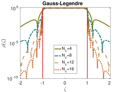
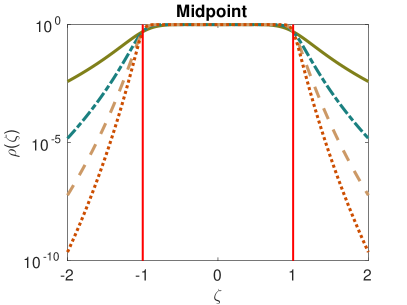
Fig. 1: The modulus of the rational filter function $\rho(\zeta)$ when $\zeta\in[-2,2]$. Left: Gauss-Legendre rule. Right: Midpoint rule.

Figure 1 plots the modulus of the rational function $\rho(\zeta)$ (scaled such that $\rho(\alpha)\equiv\rho(\beta)\equiv 1/2$) in the interval $\zeta\in[-2,2]$, where $\{\zeta_{\ell},\omega_{\ell}\}_{1\leq\ell\leq 2N_{c}}$ are obtained by numerically approximating $I_{[-1,1]}(\zeta)$ by the Gauss-Legendre rule (left) and Midpoint rule (right). Notice that as $N_{c}$ increases, $\rho(\zeta)$ becomes a more accurate approximation of $I_{[-1,1]}(\zeta)$ [37]. Throughout the rest of this paper, we will only consider the Midpoint rule [2].

2.2 Rational filtered Arnoldi procedure

Now, consider the rational matrix function $\rho(M^{-1}A)$ with $\rho(.)$ defined as in (2):

(4) $$\rho(M^{-1}A)=2\Re e\left\{\sum_{\ell=1}^{N_{c}}\omega_{\ell}(A-\zeta_{\ell}M)^{-1}M\right\}.$$

The eigenvectors of $\rho(M^{-1}A)$ are identical to those of $(A,M)$, while the corresponding eigenvalues are transformed to $\left\{\rho(\lambda_{j})\right\}_{j=1,\ldots,n}$. Since $\rho(\lambda_{1}),\ldots,\rho(\lambda_{nev})$ are all larger than $\rho(\lambda_{nev+1}),\ldots,\rho(\lambda_{n})$, the eigenvalues of $(A,M)$ located inside $[\alpha,\beta]$ become the dominant ones in $\rho(M^{-1}A)$. Applying a projection method to $\rho(M^{-1}A)$ can then lead to fast convergence towards an invariant subspace associated with the eigenvalues of $(A,M)$ located inside $[\alpha,\beta]$.

One popular choice as the projection method in rational filtering approaches is that of subspace iteration, e.g., as in the FEAST package [29, 21, 22]. One issue with this choice is that an estimation of $nev$ needs be provided in order to determine the dimension of the starting subspace. In this paper, we exploit Krylov subspace methods to avoid the requirement of providing an estimation of $nev$.

Algorithm 2.1.

RF-KRYLOV

0.	Start with $q^{(1)}\in\mathbb{R}^{n}\ s.t.\ \|q^{(1)}\|_{2}=1$
1.	For $\mu=1,2,\ldots$
2.		Compute $w=2\Re e\left\{\sum_{\ell=1}^{N_{c}}\omega_{\ell}(A-\zeta_{\ell}M)^{-1}Mq^{(\mu)}\right\}$
3.		For $\kappa=1,\ldots,\mu$
4.			$h_{\kappa,\mu}=w^{T}q^{(\kappa)}$
5.			$w=w-h_{\kappa,\mu}q^{(\kappa)}$
6.		End
7.		$h_{\mu+1,\mu}=\|w\|_{2}$
8.		If $h_{\mu+1,\mu}=0$
9.			generate a unit-norm $q^{(\mu+1)}$ orthogonal to $q^{(1)},\ldots,q^{(\mu)}$
10.		Else
11.			$q^{(\mu+1)}=w/h_{\mu+1,\mu}$
12		EndIf
13.		If the sum of eigenvalues of $H_{\mu}$ no less than $1/2$ is unchanged
		during the last few iterations; BREAK; EndIf
14.	End
15.	Compute the eigenvectors of $H_{\mu}$ and form the Ritz vectors of $(A,M)$
16.	For each Ritz vector $\hat{q}$, compute the corresponding approximate
	Ritz value as the Rayleigh quotient $\hat{q}^{T}A\hat{q}/\hat{q}^{T}M\hat{q}$

Algorithm 2.1 sketches the Arnoldi procedure applied to $\rho(M^{-1}A)$ for the computation of all eigenvalues of $(A,M)$ located inside $[\alpha,\beta]$ and associated eigenvectors. Line 2 computes the “filtered” vector $w$ by applying the matrix function $\rho(M^{-1}A)$ to $q^{(\mu)}$, which in turn requires the solution of the $N_{c}$ linear systems associated with matrices $A-\zeta_{\ell}M,\ \ell=1,\ldots,N_{c}$. Lines 3-12 orthonormalize $w$ against the previous Arnoldi vectors $q^{(1)},\ldots,q^{(\mu)}$ to produce the next Arnoldi vector $q^{(\mu+1)}$. Line 13 checks the sum of those eigenvalues of the upper-Hessenberg matrix $H_{\mu}$ which are no less than $1/2$. If this sum remains constant up to a certain tolerance, the outer loop stops. Finally, line 16 computes the Rayleigh quotients associated with the approximate eigenvectors of $\rho(M^{-1}A)$ (the Ritz vectors obtained in line 15).

Throughout the rest of this paper, Algorithm 2.1 will be abbreviated as RF-KRYLOV.

2.3 Domain decomposition framework

Domain decomposition eigenvalue solvers [18, 19, 10, 9] compute spectral information of $(A,M)$ by decoupling the original eigenvalue problem into two separate subproblems: one defined locally in the interior of each subdomain, and one restricted to the interface region connecting neighboring subdomains. Algebraic domain decomposition eigensolvers start by calling a graph partitioner [27, 20] to decompose the adjacency graph of $|A|+|M|$ into $p$ non-overlapping subdomains. If we then order the interior variables in each subdomain before the interface variables across all subdomains, matrices ${A}$ and ${M}$ then take the following block structures:

(5) $$A=\begin{pmatrix}B_{1}&&&&E_{1}\cr&B_{2}&&&E_{2}\cr&&\ddots&&\vdots\cr&&&B_{p}&E_{p}\cr E_{1}^{T}&E_{2}^{T}&\ldots&E_{p}^{T}&C\cr\end{pmatrix},\ \ \ M=\begin{pmatrix}M_{B}^{(1)}&&&&M_{E}^{(1)}\cr&M_{B}^{(2)}&&&M_{E}^{(2)}\cr&&\ddots&&\vdots\cr&&&M_{B}^{(p)}&M_{E}^{(p)}\cr M_{E}^{(1)T}&M_{E}^{(2)T}&\ldots&M_{E}^{(p)T}&M_{C}\cr\end{pmatrix}.$$

If we denote the number of interior and interface variables lying in the $j$th subdomain by $d_{j}$ and $s_{j}$, respectively, and set $s=\sum_{j=1}^{p}s_{j}$, then $B_{j}$ and $M_{B}^{(j)}$ are square matrices of size $d_{j}\times d_{j}$, $E_{j}$ and $M_{E}^{(j)}$ are rectangular matrices of size $d_{j}\times s_{j}$, and $C$ and $M_{C}$ are square matrices of size $s\times s$. Matrices $E_{i},\ M_{E}^{(j)}$ have a special nonzero pattern of the form $E_{j}=[0_{d_{j},\ell_{j}},\hat{E}_{j},0_{d_{j},\nu_{j}}]$, and $M_{E}^{(j)}=[0_{d_{j},\ell_{j}},\hat{M}_{E}^{(j)},0_{d_{j},\nu_{j}}]$, where $\ell_{j}=\sum_{k=1}^{k<j}s_{k}$, $\nu_{j}=\sum_{k>j}^{k=p}s_{k}$, and $0_{\chi,\psi}$ denotes the zero matrix of size $\chi\times\psi$.

Under the permutation (5), $A$ and $M$ can be also written in a compact form as:

(6) $$A=\begin{pmatrix}B&E\cr E^{T}&C\end{pmatrix},\ \ \ M=\begin{pmatrix}M_{B}&M_{E}\cr M_{E}^{T}&M_{C}\end{pmatrix}.$$

The block-diagonal matrices $B$ and $M_{B}$ are of size $d\times d$, where $d=\sum_{i=1}^{p}d_{i}$, while $E$ and $M_{E}$ are of size $d\times s$.

2.3.1 Invariant subspaces from a Schur complement viewpoint

Domain decomposition eigenvalue solvers decompose the construction of the Rayleigh-Ritz projection subspace ${\cal Z}$ is formed by two separate parts. More specifically, ${\cal Z}$ can be written as

(7) $${\cal Z}={\cal U}\oplus{\cal Y},$$

where ${\cal U}$ and ${\cal Y}$ are subspaces that are orthogonal to each other and approximate the part of the solution associated with the interior and interface variables, respectively.

Let the $i$th eigenvector of $(A,M)$ be partitioned as

(8) $$x^{(i)}=\begin{pmatrix}u^{(i)}\\[3.00003pt] y^{(i)}\\[3.00003pt] \end{pmatrix},\ i=1,\ldots,n,$$

where $u^{(i)}\in\mathbb{R}^{d}$ and $y^{(i)}\in\mathbb{R}^{s}$ correspond to the eigenvector part associated with the interior and interface variables, respectively. We can then rewrite $Ax^{(i)}=\lambda_{i}Mx^{(i)}$ in the following block form

(9) $$\begin{pmatrix}B-\lambda_{i}M_{B}&E-\lambda_{i}M_{E}\\[3.00003pt] E^{T}-\lambda_{i}M_{E}^{T}&C-\lambda_{i}M_{C}\\[3.00003pt] \end{pmatrix}\begin{pmatrix}u^{(i)}\\[3.00003pt] y^{(i)}\\[3.00003pt] \end{pmatrix}=0.$$

Eliminating $u^{(i)}$ from the second equation in (9) leads to the following nonlinear eigenvalue problem of size $s\times s$:

(10) $$[C-\lambda_{i}M_{C}-(E-\lambda_{i}M_{E})^{T}(B-\lambda_{i}M_{B})^{-1}(E-\lambda_{i}M_{E})]y^{(i)}=0.$$

Once $y^{(i)}$ is computed in the above equation, $u^{(i)}$ can be recovered by the following linear system solution

(11) $$(B-\lambda_{i}M_{B})u^{(i)}=-(E-\lambda_{i}M_{E})y^{(i)}.$$

In practice, since matrices $B$ and $M_{B}$ in (5) are block-diagonal, the $p$ sub-vectors $u_{j}^{(i)}\in\mathbb{R}^{d_{j}}$ of $u^{(i)}=[(u_{1}^{(i)})^{T},\ldots,(u_{p}^{(i)})^{T}]^{T}$ can be computed in a decoupled fashion among the $p$ subdomains as

(12) $$(B_{j}-\lambda_{i}M_{B}^{(j)})u_{j}^{(i)}=-(\hat{E}_{j}-\lambda_{i}\hat{M}_{E}^{(j)})y_{j}^{(i)},\ j=1,\ldots,p,$$

where $y_{j}^{(i)}\in\mathbb{R}^{s_{j}}$ is the subvector of $y^{(i)}=[(y_{1}^{(i)})^{T},\ldots,(y_{p}^{(i)})^{T}]^{T}$ that corresponds to the $j$th subdomain.

By (10) and (11) we see that the subspaces ${\cal U}$ and ${\cal Y}$ in (7) should ideally be chosen as

(13) $${\cal Y}={\rm span}\left\{\left[y^{(1)},\ldots,y^{(nev)}\right]\right\},$$

(14) $${\cal U}={\rm span}\left\{\left[(B-\lambda_{1}M_{B})^{-1}(E-\lambda_{1}M_{E})y^{(1)},\ldots,(B-\lambda_{nev}M_{B})^{-1}(E-\lambda_{nev}M_{E})y^{(nev)}\right]\right\}.$$

The following two sections propose efficient numerical schemes to approximate these two subspaces.

3 Approximation of $\operatorname{span}\{y^{(1)},\ldots,y^{(nev)}\}$

In this section we propose a numerical scheme to approximate $\operatorname{span}\{y^{(1)},\ldots,y^{(nev)}\}$.

3.1 Rational filtering restricted to the interface region

Let us define the following matrices:

$$B_{\zeta_{\ell}}=B-\zeta_{\ell}M_{B}, E_{\zeta_{\ell}}=E-\zeta_{\ell}M_{E}, \ \ C_{\zeta_{\ell}}=C-\zeta_{\ell}M_{C}.$$

Then, each matrix $(A-\zeta_{\ell}M)^{-1}$ in (4) can be expressed as

(15) $$(A-\zeta_{\ell}M)^{-1}=\begin{pmatrix}B_{\zeta_{\ell}}^{-1}+B_{\zeta_{\ell}}^{-1}E_{\zeta_{\ell}}S_{\zeta_{\ell}}^{-1}E_{\zeta_{\ell}}^{H}B_{\zeta_{\ell}}^{-1}&-B_{\zeta_{\ell}}^{-1}E_{\zeta_{\ell}}S_{\zeta_{\ell}}^{-1}\\[3.00003pt] -S_{\zeta_{\ell}}^{-1}E_{\zeta_{\ell}}^{H}B_{\zeta_{\ell}}^{-1}&S_{\zeta_{\ell}}^{-1}\\[3.00003pt] \end{pmatrix},$$

where

(16) $$S_{\zeta_{\ell}}=C_{\zeta_{\ell}}-E_{\zeta_{\ell}}^{H}B_{\zeta_{\ell}}^{-1}E_{\zeta_{\ell}},$$

denotes the corresponding Schur complement matrix.

Substituting (15) into (4) leads to

(17) $$\rho(M^{-1}A)= 2\Re e\left\{\sum_{\ell=1}^{N_{c}}\omega_{\ell}\begin{bmatrix}\left[B_{\zeta_{\ell}}^{-1}+B_{\zeta_{\ell}}^{-1}E_{\zeta_{\ell}}S_{\zeta_{\ell}}^{-1}E_{\zeta_{\ell}}^{H}B_{\zeta_{\ell}}^{-1}\right]&-B_{\zeta_{\ell}}^{-1}E_{\zeta_{\ell}}S_{\zeta_{\ell}}^{-1}\\[3.00003pt] -S_{\zeta_{\ell}}^{-1}E_{\zeta_{\ell}}^{H}B_{\zeta_{\ell}}^{-1}&S_{\zeta_{\ell}}^{-1}\\[3.00003pt] \end{bmatrix}\right\}M.$$

On the other hand, we have for any $\zeta\notin\Lambda(A,M)$:

(18) $$(A-\zeta M)^{-1}=\sum_{i=1}^{n}\dfrac{x^{(i)}(x^{(i)})^{T}}{\lambda_{i}-\zeta}.$$

The above equality yields another expression for $\rho(M^{-1}A)$:

(19) $$\rho(M^{-1}A) =\sum_{i=1}^{n}\rho(\lambda_{i})x^{(i)}(x^{(i)})^{T}M$$

(20) $$=\sum_{i=1}^{n}\rho(\lambda_{i})\begin{bmatrix}u^{(i)}(u^{(i)})^{T}&u^{(i)}(y^{(i)})^{T}\\[3.00003pt] y^{(i)}(u^{(i)})^{T}&y^{(i)}(y^{(i)})^{T}\end{bmatrix}M.$$

Equating the (2,2) blocks of the right-hand sides in (17) and (20), yields

(21) $$2\Re e\left\{\sum_{\ell=1}^{N_{c}}\omega_{\ell}S_{\zeta_{\ell}}^{-1}\right\}=\sum_{i=1}^{n}\rho(\lambda_{i})y^{(i)}(y^{(i)})^{T}.$$

Equation (21) provides a way to approximate $\operatorname{span}\{y^{(1)},\ldots,y^{(nev)}\}$ through the information in $S_{\zeta_{\ell}}^{-1}$. The coefficient $\rho(\lambda_{i})$ can be interpreted as the contribution of the direction $y^{(i)}$ in $2\Re e\left\{\sum_{\ell=1}^{N_{c}}\omega_{\ell}S_{\zeta_{\ell}}^{-1}\right\}$. In the ideal case where $\rho(\zeta)\equiv\pm I_{[\alpha,\beta]}(\zeta)$, we have $\sum_{i=1}^{n}\rho(\lambda_{i})y^{(i)}(y^{(i)})^{T}=\pm\sum_{i=1}^{nev}y^{(i)}(y^{(i)})^{T}$. In practice, $\rho(\zeta)$ will only be an approximation to $\pm I_{[\alpha,\beta]}(\zeta)$, and since $\rho(\lambda_{1}),\ldots,\rho(\lambda_{nev})$ are all nonzero, the following relation holds:

(22) $${\rm span}\{y^{(1)},\ldots,y^{(nev)}\}\subseteq{\rm range}\left(\Re e\left\{\sum_{\ell=1}^{N_{c}}\omega_{\ell}S_{\zeta_{\ell}}^{-1}\right\}\right).$$

The above relation suggests to compute an approximation to $\operatorname{span}\{y^{(1)},\ldots,y^{(nev)}\}$ by capturing the range space of $\Re e\left\{\sum_{\ell=1}^{N_{c}}\omega_{\ell}S_{\zeta_{\ell}}^{-1}\right\}$.

3.2 A Krylov-based approach

To capture ${\rm range}\left(\Re e\left\{\sum_{\ell=1}^{N_{c}}\omega_{\ell}S_{\zeta_{\ell}}^{-1}\right\}\right)$ we consider the numerical scheme outlined in Algorithm 3.1. In contrast with RF-KRYLOV, Algorithm 3.1 is based on the Lanczos process [31]. Variable $T_{\mu}$ denotes a $\mu\times\mu$ symmetric tridiagonal matrix with $\alpha_{1},\ldots,\alpha_{\mu}$ as its diagonal entries, and $\beta_{1},\ldots,\beta_{\mu-1}$ as its off-diagonal entries, respectively. Line 2 computes the “filtered” vector $w$ by applying $\Re e\left\{\sum_{\ell=1}^{N_{c}}\omega_{\ell}S_{\zeta_{\ell}}^{-1}\right\}$ to $q^{(\mu)}$ by solving the $N_{c}$ linear systems associated with matrices $S_{\zeta_{\ell}},\ \ell=1,\ldots,N_{c}$. Lines 4-12 orthonormalize $w$ against vectors $q^{(1)},\ldots,q^{(\mu)}$ in order to generate the next vector $q^{(\mu+1)}$. Algorithm 3.1 terminates when the trace of the tridiagonal matrices $T_{\mu}$ and $T_{\mu-1}$ remains the same up to a certain tolerance.

Algorithm 3.1.

Krylov restricted to the interface variables

0.	Start with $q^{(1)}\in\mathbb{R}^{s},\ s.t.\ \|q^{(1)}\|_{2}=1,$ $q_{0}:=0,$ $b_{1}=0$, ${\rm tol}\in\mathbb{R}$
1.	For $\mu=1,2,\ldots$
2.		Compute $w=\Re e\left\{\sum_{\ell=1}^{N_{c}}\omega_{\ell}S_{\zeta_{\ell}}^{-1}q^{(\mu)}\right\}-b_{\mu}q^{(\mu-1)}$
3.		$a_{\mu}=w^{T}q^{(\mu)}$
4.		For $\kappa=1,\ldots,\mu$
5.			$w=w-q^{(\kappa)}(w^{T}q^{(\kappa)})$
6.		End
7.		$b_{\mu+1}:=\|w\|_{2}$
8.		If $b_{\mu+1}=0$
9.			generate a unit-norm $q^{(\mu+1)}$ orthogonal to $q^{(1)},\ldots,q^{(\mu)}$
10.		Else
11.			$q^{(\mu+1)}=w/b_{\mu+1}$
12		EndIf
13.		If the sum of eigenvalue of $T_{\mu}$ remains unchanged (up to ${\rm tol}$)
		during the last few iterations; BREAK; EndIf
14.	End
15.	Return $Q_{\mu}=[q^{(1)},\ldots,q^{(\mu)}]$

Algorithm 3.1 and RF-KRYLOV share a few key differences. First, Algorithm 3.1 restricts orthonormalization to vectors of length $s$ instead of $n$. In addition, Algorithm 3.1 only requires linear system solutions with $S_{\zeta}$ instead of $A-\zeta M$. As can be verified by (15), a computation of the form $(A-\zeta M)^{-1}v=w,\ \zeta\in\mathbb{C}$ requires -in addition to a linear system solution with matrix $S_{\zeta}$- two linear system solutions with $B_{\zeta}$ as well as two Matrix-Vector multiplications with $E_{\zeta}$. Finally, in contrast to RF-KRYLOV which requires at least $nev$ iterations to compute any $nev$ eigenpairs of the pencil $(A,M)$, Algorithm 3.1 might terminate in fewer than $nev$ iterations. This possible “early termination” of Algorithm 3.1 is explained in more detail by Proposition 1.

Proposition 1.

The rank of the matrix $\Re e\left\{\sum_{\ell=1}^{N_{c}}\omega_{\ell}S_{\zeta_{\ell}}^{-1}\right\}$,

(23) $$r(S)={\rm rank}\left(\Re e\left\{\sum_{\ell=1}^{N_{c}}\omega_{\ell}S_{\zeta_{\ell}}^{-1}\right\}\right),$$

satisfies the inequality

(24) $${\rm rank}\left(\left[y^{(1)},\ldots,y^{(nev)}\right]\right)\leq r(S)\leq s.$$

Proof.

We first prove the upper bound of $r(S)$. Since $\Re e\left\{\sum_{\ell=1}^{N_{c}}\omega_{\ell}S_{\zeta_{\ell}}^{-1}\right\}$ is of size $s\times s$, $r(S)$ can not exceed $s$. To get the lower bound, let $\rho(\lambda_{i})=0,\ i=nev+\kappa,\ldots,n$, where $0\leq\kappa\leq n-nev$. We then have

$$\Re e\left\{\sum_{\ell=1}^{N_{c}}\omega_{\ell}S_{\zeta_{\ell}}^{-1}\right\}=\sum_{i=1}^{nev+\kappa}\rho(\lambda_{i})y^{(i)}(y^{(i)})^{T},$$

and ${\rm rank}\left(\Re e\left\{\sum_{\ell=1}^{N_{c}}\omega_{\ell}S_{\zeta_{\ell}}^{-1}\right\}\right)={\rm rank}\left(\left[y^{(1)},\ldots,y^{(nev+\kappa)}\right]\right)$. Since $\rho(\lambda_{i})\neq 0,\ i=1,\ldots,nev$, we have

$$r(S)={\rm rank}\left(\left[y^{(1)},\ldots,y^{(nev+\kappa)}\right]\right)\geq{\rm rank}\left(\left[y^{(1)},\ldots,y^{(nev)}\right]\right).$$

∎

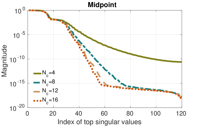
Fig. 2: The leading singular values of $\Re e\left\{\sum_{\ell=1}^{N_{c}}\omega_{\ell}S_{\zeta_{\ell}}^{-1}\right\}$ for different values of $N_{c}$.

By Proposition 1, Algorithm 3.1 will perform at most $r(S)$ iterations, and $r(S)$ can be as small as ${\rm rank}\left(\left[y^{(1)},\ldots,y^{(nev)}\right]\right)$. We quantify this with a short example for a 2D Laplacian matrix generated by a Finite Difference discretization with Dirichlet boundary conditions (for more details on this matrix see entry “FDmesh1” in Table 1) where we set $[\alpha,\beta]=[\lambda_{1},\lambda_{100}]$ (thus $nev=100$). After computing vectors $y^{(1)},\ldots,y^{(nev)}$ explicitly, we found that ${\rm rank}\left(\left[y^{(1)},\ldots,y^{(nev)}\right]\right)=48$. Figure 2 plots the 120 (after normalization) leading singular values of matrix $\Re e\left\{\sum_{\ell=1}^{N_{c}}\omega_{\ell}S_{\zeta_{\ell}}^{-1}\right\}$. As $N_{c}$ increases, the trailing $s-{\rm rank}\left(\left[y^{(1)},\ldots,y^{(nev)}\right]\right)$ singular values approach zero. Moreover, even for those singular values which are not zero, their magnitude might be small, in which case Algorithm 3.1 might still converge in fewer than $r(S)$ iterations. Indeed, when $N_{c}=16$, Algorithm 3.1 terminates after exactly $36$ iterations which is lower than $r(S)$ and only one third of the minimum number of iterations required by RF-KRYLOV for any value of $N_{c}$. As a sidenote, when $N_{c}=2$, Algorithm 3.1 terminates after $70$ iterations.

4 Approximation of $\operatorname{span}\{u^{(1)},\ldots,u^{(nev)}\}$

Recall the partitioning of eigenvector $x^{(i)}$ in (8) and assume that its interface part $y^{(i)}$ is already computed. A straightforward approach to recover $u^{(i)}$ is then to solve the linear system in $(\ref{schur_eigvec2})$. However, this entails two drawbacks. First, solving the linear systems with each different $B-\lambda_{i}M_{B}$ for all $\lambda_{i},\ i=1,\ldots,nev$ might become prohibitively expensive when $nev\gg 1$. More importantly, Algorithm 3.1 only returns an approximation to ${\rm span}\{y^{(1)},\ldots,y^{(nev)}\}$, rather than the individual vectors $y^{(1)},\ldots,y^{(nev)}$, or the eigenvalues $\lambda_{1},\ldots,\lambda_{nev}$.

In this section we alternatives for the approximation of ${\rm span}\left\{u^{(1)},\ldots,u^{(nev)}\right\}$. Since the following discussion applies to all $n$ eigenpairs of $(A,M)$, we will drop the superscripts in $u^{(i)}$ and $y^{(i)}$.

4.1 The basic approximation

To avoid solving the $nev$ different linear systems in $(\ref{schur_eigvec2})$ we consider the same real scalar $\sigma$ for all $nev$ sought eigenpairs. The part of each sought eigenvector $x$ corresponding to the interior variables, $u$, can then be approximated by

(25) $$\hat{u}=-B_{\sigma}^{-1}E_{\sigma}y.$$

In the following proposition, we analyze the difference between $u$ and its approximation $\hat{u}$ obtained by (25).

Lemma 2.

Suppose $u$ and $\hat{u}$ are computed as in $(\ref{schur_eigvec2})$ and $(\ref{prol2})$, respectively.

Then:

(26) $$u-\hat{u}=-[B_{\lambda}^{-1}-B_{\sigma}^{-1}]E_{\sigma}y+(\lambda-\sigma)B_{\lambda}^{-1}M_{E}y.$$

Proof.

We can write $u$ as

(27) $$u =-B_{\lambda}^{-1}E_{\lambda}y$$

$$=-B_{\lambda}^{-1}(E_{\sigma}-(\lambda-\sigma)M_{E})y$$

$$=-B_{\lambda}^{-1}E_{\sigma}y+(\lambda-\sigma)B_{\lambda}^{-1}M_{E}y.$$

The result in (26) follows by combining (25) and (27). ∎

We are now ready to compute an upper bound of $u-\hat{u}$ measured in the $M_{B}$-norm.

Theorem 3.

Let the eigendecomposition of $(B,M_{B})$ be written as

(28) $$BV=M_{B}VD,$$

where $D={\rm diag}(\delta_{1},\ldots,\delta_{d})$ and $V=[v^{(1)},\ldots,v^{(d)}]$. If $\hat{u}$ is defined as in (25) and $(\delta_{\ell},v^{(\ell)}),\ \ell=1,\ldots,d$ denote the eigenpairs of $(B,M_{B})$ with $(v^{(\ell)})^{T}M_{B}v^{(\ell)}=1$, then

(29) $$\left\|u-\hat{u}\right\|_{M_{B}}\leq\max_{\ell}\frac{|\lambda-\sigma|}{|(\lambda-\delta_{\ell})(\sigma-\delta_{\ell})|}||E_{\sigma}y||_{M^{-1}_{B}}+\max_{\ell}\frac{|\lambda-\sigma|}{|\lambda-\delta_{\ell}|}||M_{E}y||_{M^{-1}_{B}},$$

Proof.

Since $M_{B}$ is SPD, vectors $E_{\sigma}y$ and $M_{E}y$ in (27) can be expanded in the basis $M_{B}v^{(\ell)}$ as:

(30) $$E_{\sigma}y=M_{B}\sum_{\ell=1}^{\ell=d}\epsilon_{\ell}v^{(\ell)},\ \ \ M_{E}y=M_{B}\sum_{\ell=1}^{\ell=d}\gamma_{\ell}v^{(\ell)},$$

where $\epsilon_{\ell},\ \gamma_{\ell}\in\mathbb{R}$ are the expansion coefficients. Based on (28) and noting that $V^{T}M_{B}V=I$, shows that

(31) $$B_{\sigma}^{-1}=V(D-\sigma I)^{-1}V^{T},\ \ \ B_{\lambda}^{-1}=V(D-\lambda I)^{-1}V^{T}.$$

Substituting $(\ref{carousel2})$ and $(\ref{eq:bb})$ into the right-hand side of (26) gives

$$u-\hat{u}= -V\left[(D-\lambda I)^{-1}-(D-\sigma I)^{-1}\right]V^{T}\left(M_{B}\sum_{\ell=1}^{\ell=d}\epsilon_{\ell}v^{(\ell)}\right)$$

$$+(\lambda-\sigma)V(D-\lambda I)^{-1}V^{T}\left(M_{B}\sum_{\ell=1}^{\ell=d}\gamma_{\ell}v^{(\ell)}\right)$$

$$= -\sum_{\ell=1}^{\ell=d}\frac{\epsilon_{\ell}(\lambda-\sigma)}{(\delta_{\ell}-\lambda)(\delta_{\ell}-\sigma)}v^{(\ell)}+\sum_{\ell=1}^{\ell=d}\frac{\gamma_{\ell}(\lambda-\sigma)}{\delta_{\ell}-\lambda}v^{(\ell)}.$$

Now, taking the $M_{B}$-norm of the above equation, we finally obtain

$$||u-\hat{u}||_{M_{B}} \leq\left\|\sum_{\ell=1}^{\ell=d}\frac{\epsilon_{\ell}(\lambda-\sigma)}{(\delta_{\ell}-\lambda)(\delta_{\ell}-\sigma)}v^{(\ell)}\right\|_{M_{B}}+\left\|\sum_{\ell=1}^{\ell=d}\frac{\gamma_{\ell}(\lambda-\sigma)}{\delta_{\ell}-\lambda}v^{(\ell)}\right\|_{M_{B}}$$

$$=\left\|\sum_{\ell=1}^{\ell=d}\left|\frac{(\lambda-\sigma)}{(\delta_{\ell}-\lambda)(\delta_{\ell}-\sigma)}\right|\epsilon_{\ell}v^{(\ell)}\right\|_{M_{B}}+\left\|\sum_{\ell=1}^{\ell=d}\left|\frac{(\lambda-\sigma)}{\delta_{\ell}-\lambda}\right|\gamma_{\ell}v^{(\ell)}\right\|_{M_{B}}$$

$$\leq\max_{\ell}\frac{|\lambda-\sigma|}{|(\lambda-\delta_{\ell})(\sigma-\delta_{\ell})|}\left\|\sum_{\ell=1}^{\ell=d}\epsilon_{\ell}v^{(\ell)}\right\|_{M_{B}}+\max_{\ell}\frac{|\lambda-\sigma|}{|\lambda-\delta_{\ell}|}\left\|\sum_{\ell=1}^{\ell=d}\gamma_{\ell}v^{(\ell)}\right\|_{M_{B}}$$

$$=\max_{\ell}\frac{|\lambda-\sigma|}{|(\lambda-\delta_{\ell})(\sigma-\delta_{\ell})|}\left\|M^{-1}_{B}E_{\sigma}y\right\|_{M_{B}}+\max_{\ell}\frac{|\lambda-\sigma|}{|\lambda-\delta_{\ell}|}\left\|M^{-1}_{B}M_{E}y\right\|_{M_{B}}$$

$$=\max_{\ell}\frac{|\lambda-\sigma|}{|(\lambda-\delta_{\ell})(\sigma-\delta_{\ell})|}\left\|E_{\sigma}y\right\|_{M^{-1}_{B}}+\max_{\ell}\frac{|\lambda-\sigma|}{|\lambda-\delta_{\ell}|}\left\|M_{E}y\right\|_{M^{-1}_{B}}.$$

∎

Theorem 3 indicates that the upper bound of $||u-\hat{u}||_{M_{B}}$ depends on the distance between $\sigma$ and $\lambda$, as well as the distance of these values from the eigenvalues of $(B,M_{B})$. This upper bound becomes relatively large when $\lambda$ is located far from $\sigma$, while, on the other hand, becomes small when $\lambda$ and $\sigma$ lie close to each other, and far from the eigenvalues of $(B,M_{B})$.

4.2 Enhancing accuracy by resolvent expansions

Consider the resolvent expansion of $B_{\lambda}^{-1}$ around $\sigma$:

(32) $$B_{\lambda}^{-1}=B_{\sigma}^{-1}\sum_{\theta=0}^{\infty}\left[(\lambda-\sigma)M_{B}B_{\sigma}^{-1}\right]^{\theta}.$$

By (26), the error $u-\hat{u}$ consists of two components: $i$) $(B_{\lambda}^{-1}-B_{\sigma}^{-1})E_{\sigma}y$; and $ii$) $(\lambda-\sigma)B_{\lambda}^{-1}M_{E}y$. An immediate improvement is then to approximate $B_{\lambda}^{-1}$ by also considering higher-order terms in (32) instead of $B_{\sigma}^{-1}$ only. Furthermore, the same idea can be repeated for the second error component. Thus, we can extract $\hat{u}$ by a projection step from the following subspace

(33) $$\hat{u}\in\{B^{-1}_{\sigma}E_{\sigma}y,\ldots,B^{-1}_{\sigma}\left(M_{B}B_{\sigma}^{-1}\right)^{\psi-1}E_{\sigma}y,B^{-1}_{\sigma}M_{E}y,\ldots,B^{-1}_{\sigma}\left(M_{B}B_{\sigma}^{-1}\right)^{\psi-1}M_{E}y\}.$$

The following theorem refines the upper bound of $\|u-\hat{u}\|_{M_{B}}$ when $\hat{u}$ is approximated by the subspace in (33) and $\psi\geq 1$ resolvent expansion terms are retained in (32).

Theorem 4.

Let ${\cal U}={\rm span}\left\{U_{1},U_{2}\right\}$ where

(34) $$U_{1}=\left[B_{\sigma}^{-1}E_{\sigma}y,\ldots,B_{\sigma}^{-1}\left(M_{B}B_{\sigma}^{-1}\right)^{\psi-1}E_{\sigma}y\right],$$

(35) $$U_{2}=\left[B_{\sigma}^{-1}M_{E}y,\ldots,B_{\sigma}^{-1}\left(M_{B}B_{\sigma}^{-1}\right)^{\psi-1}M_{E}y\right].$$

If $\hat{u}:=\operatornamewithlimits{arg\,min}_{g\in{\cal U}}\|u-g\|_{M_{B}}$, and $(\delta_{\ell},v^{(\ell)}),\ \ell=1,\ldots,d$ denote the eigenpairs of $(B,M_{B})$, then:

(36) $$\|u-\hat{u}\|_{M_{B}}\leq\max_{\ell}\frac{|\lambda-\sigma|^{\psi}||E_{\sigma}y||_{M^{-1}_{B}}}{|(\lambda-\delta_{\ell})(\sigma-\delta_{\ell})^{\psi}|}+\max_{\ell}\frac{|\lambda-\sigma|^{\psi+1}||M_{E}y||_{M^{-1}_{B}}}{|(\lambda-\delta_{\ell})(\sigma-\delta_{\ell})^{\psi}|}.$$

Proof.

Define a vector $g:=U_{1}{\bf c}_{1}+U_{2}{\bf c}_{2}$ where

(37) $${\bf c}_{1}=-\left[1,\lambda-\sigma,\ldots,(\lambda-\sigma)^{\psi-1}\right]^{T},\ \ \ {\bf c}_{2}=\left[\lambda-\sigma,\ldots,(\lambda-\sigma)^{\psi}\right]^{T}.$$

If we equate terms, the difference between $u$ and $g$ satisfies

(38) $$u-g= -\left[B_{\lambda}^{-1}-B_{\sigma}^{-1}\sum_{\theta=0}^{\psi-1}\left[(\lambda-\sigma)M_{B}B_{\sigma}^{-1}\right]^{\theta}\right]E_{\sigma}y$$

$$+(\lambda-\sigma)\left[B_{\lambda}^{-1}-B_{\sigma}^{-1}\sum_{\theta=0}^{\psi-1}\left[(\lambda-\sigma)M_{B}B_{\sigma}^{-1}\right]^{\theta}\right]M_{E}y.$$

Expanding $B_{\sigma}^{-1}$ and $B_{\lambda}^{-1}$ in the eigenbasis of $(B,M_{B})$ gives

(39) $$B_{\lambda}^{-1}-B_{\sigma}^{-1}\sum_{\theta=0}^{\psi-1}\left[(\lambda-\sigma)M_{B}B_{\sigma}^{-1}\right]^{\theta} =(\lambda-\sigma)^{\psi}\left[V(D-\lambda I)^{-1}(D-\sigma I)^{-\psi}V^{T}\right],$$

and thus (38) can be simplified as

$$u-g= -(\lambda-\sigma)^{\psi}V(D-\lambda I)^{-1}(D-\sigma I)^{-\psi}V^{T}E_{\sigma}y$$

$$\ +(\lambda-\sigma)^{\psi+1}V(D-\lambda I)^{-1}(D-\sigma I)^{-\psi}V^{T}M_{E}y.$$

Plugging in the expansion of $E_{\sigma}y$ and $M_{E}y$ defined in (30) finally leads to

(40) $$u-g=\sum_{\ell=1}^{\ell=d}\dfrac{-\epsilon_{\ell}(\lambda-\sigma)^{\psi}}{(\delta_{\ell}-\lambda)(\delta_{\ell}-\sigma)^{\psi}}v^{(\ell)}+\sum_{\ell=1}^{\ell=d}\dfrac{\gamma_{\ell}(\lambda-\sigma)^{\psi+1}}{(\delta_{\ell}-\lambda)(\delta_{\ell}-\sigma)^{\psi}}v^{(\ell)}.$$

Considering the $M_{B}$-norm gives

$$\|u-g\|_{M_{B}} \leq\left\|\sum_{\ell=1}^{\ell=d}\dfrac{-\epsilon_{\ell}(\lambda-\sigma)^{\psi}}{(\delta_{\ell}-\lambda)(\delta_{\ell}-\sigma)^{\psi}}v^{(\ell)}\right\|_{M_{B}}+\left\|\sum_{\ell=1}^{\ell=d}\dfrac{\gamma_{\ell}(\lambda-\sigma)^{\psi+1}}{(\delta_{\ell}-\lambda)(\delta_{\ell}-\sigma)^{\psi}}v^{(\ell)}\right\|_{M_{B}}$$

$$\leq\max_{\ell}\frac{|\lambda-\sigma|^{\psi}}{|(\lambda-\delta_{\ell})(\sigma-\delta_{\ell})^{\psi}|}\left\|\sum_{\ell=1}^{\ell=d}\epsilon_{\ell}v^{(\ell)}\right\|_{M_{B}}$$

$$\quad+\max_{\ell}\frac{|\lambda-\sigma|^{\psi+1}}{|(\lambda-\delta_{\ell})(\sigma-\delta_{\ell})^{\psi}|}\left\|\sum_{\ell=1}^{\ell=d}\gamma_{\ell}v^{(\ell)}\right\|_{M_{B}}$$

$$=\max_{\ell}\frac{|\lambda-\sigma|^{\psi}||E_{\sigma}y||_{M^{-1}_{B}}}{|(\lambda-\delta_{\ell})(\sigma-\delta_{\ell})^{\psi}|}+\max_{\ell}\frac{|\lambda-\sigma|^{\psi+1}||M_{E}y||_{M^{-1}_{B}}}{|(\lambda-\delta_{\ell})(\sigma-\delta_{\ell})^{\psi}|}.$$

Since $\hat{u}$ is the solution of $\min_{g\in{\cal U}}\|u-g\|_{M_{B}}$, it follows that $\|u-\hat{u}\|_{M_{B}}\leq\|u-g\|_{M_{B}}$. ∎

A comparison of the bound in Theorem 4 with the bound in Theorem 3 indicates that one may expect an improved approximation when $\sigma$ is close to $\lambda$. Numerical examples in Section 6 will verify that this approach enhances accuracy even when $|\sigma-\lambda|$ is not very small.

4.3 Enhancing accuracy by deflation

Both Theorem 3 and Theorem 4 imply that the approximation error $u-\hat{u}$ might have its largest components along those eigenvector directions associated with the eigenvalues of $(B,M_{B})$ located the closest to $\sigma$. We can remove these directions by augmenting the projection subspace with the corresponding eigenvectors of $(B,M_{B})$.

Theorem 5.

Let $\delta_{1},\delta_{2},\ldots,\delta_{\kappa}$ be the $\kappa$ eigenvalues of $(B,M_{B})$ that lie the closest to $\sigma$, and let $v^{(1)},v^{(2)},\ldots,v^{(\kappa)}$ denote the corresponding eigenvectors. Moreover, let ${\cal U}={\rm span}\left\{U_{1},U_{2},U_{3}\right\}$ where

(41) $$U_{1}=\left[B_{\sigma}^{-1}E_{\sigma}y,\ldots,B_{\sigma}^{-1}\left(M_{B}B_{\sigma}^{-1}\right)^{\psi-1}E_{\sigma}y\right],$$

(42) $$U_{2}=\left[B_{\sigma}^{-1}M_{E}y,\ldots,B_{\sigma}^{-1}\left(M_{B}B_{\sigma}^{-1}\right)^{\psi-1}M_{E}y\right],$$

(43) $$U_{3}=\left[v^{(1)},v^{(2)},\ldots,v^{(\kappa)}\right].$$

If $\hat{u}:=\operatornamewithlimits{arg\,min}_{g\in{\cal U}}\|u-g\|_{M_{B}}$and $(\delta_{\ell},v^{(\ell)}),\ \ell=1,\ldots,d$ denote the eigenpairs of $(B,M_{B})$, then:

(44) $$\|u-\hat{u}\|_{M_{B}}\leq\max_{\ell>\kappa}\frac{|\lambda-\sigma|^{\psi}||E_{\sigma}y||_{M^{-1}_{B}}}{|(\lambda-\delta_{\ell})(\sigma-\delta_{\ell})^{\psi}|}+\max_{\ell>\kappa}\frac{|\lambda-\sigma|^{\psi+1}||M_{E}y||_{M^{-1}_{B}}}{|(\lambda-\delta_{\ell})(\sigma-\delta_{\ell})^{\psi}|}.$$

Proof.

Let us define the vector $g:=U_{1}{\bf c}_{1}+U_{2}{\bf c}_{2}+U_{3}{\bf c}_{3}$ where

$${\bf c}_{1}=-\left[1,\lambda-\sigma,\ldots,(\lambda-\sigma)^{\psi-1}\right]^{T},\ \ \ {\bf c}_{2}=\left[\lambda-\sigma,\ldots,(\lambda-\sigma)^{\psi}\right]^{T},$$

$${\bf c}_{3}=\left[\dfrac{\gamma_{1}(\lambda-\sigma)^{\psi+1}-\epsilon_{1}(\lambda-\sigma)^{\psi}}{(\delta_{1}-\lambda)(\delta_{1}-\sigma)^{\psi}},\ldots,\dfrac{\gamma_{\kappa}(\lambda-\sigma)^{\psi+1}-\epsilon_{\kappa}(\lambda-\sigma)^{\psi}}{(\delta_{\kappa}-\lambda)(\delta_{\kappa}-\sigma)^{\psi}}\right]^{T}.$$

Since ${\bf c}_{1}$ and ${\bf c}_{2}$ are identical to those defined in (37), we can proceed as in (40) and subtract $U_{3}{\bf c}_{3}$. Then,

$$u-g= \sum_{\ell=1}^{\ell=d}\dfrac{-\epsilon_{\ell}(\lambda-\sigma)^{\psi}}{(\delta_{\ell}-\lambda)(\delta_{\ell}-\sigma)^{\psi}}v^{(\ell)}+\sum_{\ell=1}^{\ell=d}\dfrac{\gamma_{\ell}(\lambda-\sigma)^{\psi+1}}{(\delta_{\ell}-\lambda)(\delta_{\ell}-\sigma)^{\psi}}v^{(\ell)}$$

$$-\sum_{\ell=1}^{\ell=\kappa}\dfrac{-\epsilon_{\ell}(\lambda-\sigma)^{\psi}}{(\delta_{\ell}-\lambda)(\delta_{\ell}-\sigma)^{\psi}}v^{(\ell)}-\sum_{\ell=1}^{\ell=\kappa}\dfrac{\gamma_{\ell}(\lambda-\sigma)^{\psi+1}}{(\delta_{\ell}-\lambda)(\delta_{\ell}-\sigma)^{\psi}}v^{(\ell)}$$

$$= \sum_{\ell=\kappa+1}^{\ell=d}\dfrac{-\epsilon_{\ell}(\lambda-\sigma)^{\psi}}{(\delta_{\ell}-\lambda)(\delta_{\ell}-\sigma)^{\psi}}v^{(\ell)}+\sum_{\ell=\kappa+1}^{\ell=d}\dfrac{\gamma_{\ell}(\lambda-\sigma)^{\psi+1}}{(\delta_{\ell}-\lambda)(\delta_{\ell}-\sigma)^{\psi}}v^{(\ell)}$$

Considering the $M_{B}$-norm of $u-g$ gives

$$\left\|u-\hat{g}\right\|_{M_{B}} \leq\left\|\sum_{\ell=\kappa+1}^{\ell=d}\dfrac{-\epsilon_{\ell}(\lambda-\sigma)^{\psi}}{(\delta_{\ell}-\lambda)(\delta_{\ell}-\sigma)^{\psi}}v^{(\ell)}\right\|_{M_{B}}+\left\|\sum_{\ell=\kappa+1}^{\ell=d}\dfrac{\gamma_{\ell}(\lambda-\sigma)^{\psi+1}}{(\delta_{\ell}-\lambda)(\delta_{\ell}-\sigma)^{\psi}}v^{(\ell)}\right\|_{M_{B}}$$

$$\leq\max_{\ell>\kappa}\frac{|\lambda-\sigma|^{\psi}||E_{\sigma}y||_{M^{-1}_{B}}}{|(\lambda-\delta_{\ell})(\sigma-\delta_{\ell})^{\psi}|}+\max_{\ell>\kappa}\frac{|\lambda-\sigma|^{\psi+1}||M_{E}y||_{M^{-1}_{B}}}{|(\lambda-\delta_{\ell})(\sigma-\delta_{\ell})^{\psi}|},$$

where, as previously, we made use of the expression of $E_{\sigma}y$ and $M_{E}y$ in (30). Since $\hat{u}$ is the solution of $\min_{g\in{\cal U}}\|u-g\|_{M_{B}}$, it follows that $\|u-\hat{u}\|_{M_{B}}\leq\|u-\hat{g}\|_{M_{B}}$. ∎

5 The RF-DDES algorithm

In this section we describe RF-DDES in terms of a formal algorithm.

RF-DDES starts by calling a graph partitioner to partition the graph of $|A|+|M|$ into $p$ subdomains and reorders the matrix pencil $(A,M)$ as in (5). RF-DDES then proceeds to the computation of those eigenvectors associated with the $nev_{B}^{(j)}$ smallest (in magnitude) eigenvalues of each matrix pencil $(B_{j}-\sigma M_{B}^{(j)},M_{B}^{(j)})$, and stores these eigenvectors in $V_{j}\in\mathbb{R}^{d_{j}\times nev_{B}^{(j)}},\ j=1,\ldots,p$. As our current implementation stands, these eigenvectors are computed by Lanczos combined with shift-and-invert; see [16]. Moreover, while in this paper we do not consider any special mechanisms to set the value of $nev_{B}^{(j)}$, it is possible to adapt the work in [38]. The next step of RF-DDES is to call Algorithm 3.1 and approximate ${\rm span}\{y^{(1)},\ldots,y^{(nev)}\}$ by ${\rm range}\{Q\}$, where $Q$ denotes the orthonormal matrix returned by Algorithm 3.1. RF-DDES then builds an approximation subspace as described in Section 5.1 and performs a Rayleigh-Ritz (RR) projection to extract approximate eigenpairs of $(A,M)$. The complete procedure is shown in Algorithm 5.1.

Algorithm 5.1.

RF-DDES

0.	Input: $A,\ M,\ \alpha,\ \beta,\ \sigma,\ p,\ \{\omega_{\ell},\zeta_{\ell}\}_{\ell=1,\ldots,N_{c}},\ \{nev_{B}^{(j)}\}_{j=1,\ldots,p},\ \psi$
1.	Reorder $A$ and $M$ as in (5)
2.	For $j=1,\ldots,p$:
3.		Compute the eigenvectors associated with the $nev_{B}^{(j)}$ smallest
		(in magnitude) eigenvalues of $(B^{(j)}_{\sigma},M_{B}^{(j)})$ and store them in $V_{j}$
4.	End
5.	Compute $Q$ by Algorithm_3.1
6.	Form $Z$ as in (47)
7.	Solve the Rayleigh-Ritz eigenvalue problem: $Z^{T}AZG=Z^{T}MZG\hat{\Lambda}$
8.	If eigenvectors were also sought, permute the entries of each
	approximate eigenvector back to their original ordering

The Rayleigh-Ritz eigenvalue problem at step 7) of RF-DDES can be solved either by a shift-and-invert procedure or by the appropriate routine in LAPACK [11].

5.1 The projection matrix $Z$

Let matrix $Q$ returned by Algorithm 3.1 be written in its distributed form among the $p$ subdomains,

(45) $$Q=\begin{pmatrix}Q_{1}\\[3.00003pt] Q_{2}\\[3.00003pt] \vdots\\[3.00003pt] Q_{p}\\[3.00003pt] \end{pmatrix},$$

where $Q_{j}\in\mathbb{R}^{s_{i}\times\mu},\ j=1,\ldots,p$ is local to the $j$th subdmonain and $\mu\in\mathbb{N}^{*}$ denotes the total number of iterations performed by Algorithm 3.1. By defining

(46) $$B^{(j)}_{\sigma}=B_{j}-\sigma M_{B}^{(j)},$$

$$\Phi^{(j)}_{\sigma}=\left(E_{j}-\sigma M_{E}^{(j)}\right)Q_{j},$$

$$\Psi^{(j)}=M_{E}^{(j)}Q_{j},$$

the Rayleigh-Ritz projection matrix $Z$ in RF-DDES can be written as:

(47) $$Z=\begin{pmatrix}V_{1}&&&&-\Sigma_{1}^{(\psi)}&\Gamma_{1}^{(\psi)}\\[3.00003pt] &V_{2}&&&-\Sigma_{2}^{(\psi)}&\Gamma_{2}^{(\psi)}\\[3.00003pt] &&\ddots&&\vdots&\vdots\\[3.00003pt] &&&V_{p}&-\Sigma_{p}^{(\psi)}&\Gamma_{p}^{(\psi)}\\[3.00003pt] &&&&[Q,0_{s,(\psi-1)\mu}]&\\[3.00003pt] \end{pmatrix},$$

where $0_{\chi,\psi}$ denotes a zero matrix of size $\chi\times\psi$, and

(48) $$\Sigma_{j}^{(\psi)}=\left[(B_{\sigma}^{(j)})^{-1}\Phi^{(j)}_{\sigma},(B_{\sigma}^{(j)})^{-1}M_{B}^{(j)}(B_{\sigma}^{(j)})^{-1}\Phi^{(j)}_{\sigma},\ldots,(B_{\sigma}^{(j)})^{-1}\left(M_{B}^{(j)}(B_{\sigma}^{(j)})^{-1}\right)^{\psi-1}\Phi^{(j)}_{\sigma}\right],$$

$$\Gamma_{j}^{(\psi)}=\left[(B_{\sigma}^{(j)})^{-1}\Psi^{(j)},(B_{\sigma}^{(j)})^{-1}M_{B}^{(j)}(B_{\sigma}^{(j)})^{-1}\Psi^{(j)},\ldots,(B_{\sigma}^{(j)})^{-1}\left(M_{B}^{(j)}(B_{\sigma}^{(j)})^{-1}\right)^{\psi-1}\Psi^{(j)}\right].$$

When $M_{E}$ is a nonzero matrix, the size of matrix $Z$ is $n\times(\kappa+2\psi\mu)$. However, when $M_{E}\equiv 0_{d,s}$, as is the case for example when $M$ is the identity matrix, the size of $Z$ reduces to $n\times(\kappa+\psi\mu)$ since $\Gamma_{j}^{(\psi)}\equiv 0_{d_{j},\psi\mu}$. The total memory overhead associated with the $j$th subdomain in RF-DDES is at most that of storing $d_{j}(nev_{B}^{(j)}+2\psi\mu)+s_{i}\mu$ floating-point numbers.

5.2 Main differences with AMLS

Both RF-DDES and AMLS exploit the domain decomposition framework discussed in Section 2.3. However, the two methods have a few important differences.

In contrast to RF-DDES which exploits Algorithm 3.1, AMLS approximates the part of the solution associated with the interface variables of $(A,M)$ by solving a generalized eigenvalue problem stemming by a first-order approximation of the nonlinear eigenvalue problem in (10). More specifically, AMLS approximates ${\rm span}\left\{\left[y^{(1)},\ldots,y^{(nev)}\right]\right\}$ by the span of the eigenvectors associated with a few of the eigenvalues of smallest magnitude of the SPD pencil $(S(\sigma),-S^{\prime}(\sigma))$, where $\sigma$ is some real shift and $S^{\prime}(\sigma)$ denotes the derivative of $S(.)$ at $\sigma$. In the standard AMLS method the shift $\sigma$ is zero. While AMLS avoids the use of complex arithmetic, a large number of eigenvectors of $(S(\sigma),-S^{\prime}(\sigma))$ might need be computed. Moreover, only the span of those vectors $y^{(i)}$ for which $\lambda_{i}$ lies sufficiently close to $\sigma$ can be captured very accurately. In contrast, RF-DDES can capture all of ${\rm span}\left\{\left[y^{(1)},\ldots,y^{(nev)}\right]\right\}$ to high accuracy regardless of where $\lambda_{i}$ is located inside the interval of interest.

Another difference between RF-DDES and AMLS concerns the way in which the two schemes approximate ${\rm span}\left\{\left[u^{(1)},\ldots,u^{(nev)}\right]\right\}$. As can be easily verified, AMLS is similar to RF-DDES with the choice $\psi=1$ [9]. While it is possible to combine AMLS with higher values of $\psi$, this might not always lead to a significant increase in the accuracy of the approximate eigenpairs of $(A,M)$ due to the inaccuracies in the approximation of ${\rm span}\left\{\left[y^{(1)},\ldots,y^{(nev)}\right]\right\}$. In contrast, because RF-DDES can compute a good approximation to the entire space ${\rm span}\left\{\left[y^{(1)},\ldots,y^{(nev)}\right]\right\}$, the accuracy of the approximate eigenpairs of $(A,M)$ can be improved by simply increasing $\psi$ and/or $nev_{B}^{(j)}$ and repeating the Rayleigh-Ritz projection.

6 Experiments

In this section we present numerical experiments performed in serial and distributed memory computing environments. The RF-KRYLOV and RF-DDES schemes were written in C/C++ and built on top of the PETSc [14, 13, 6] and Intel Math Kernel (MKL) scientific libraries. The source files were compiled with the Intel MPI compiler mpiicpc, using the -O3 optimization level. For RF-DDES, the computational domain was partitioned to $p$ non-overlapping subdomains by the METIS graph partitioner [20], and each subdomain was then assigned to a distinct processor group. Communication among different processor groups was achieved by means of the Message Passing Interface standard (MPI) [33]. The linear system solutions with matrices $A-\zeta_{1}M,\ldots,A-\zeta_{N_{c}}M$ and $S(\zeta_{1}),\ldots,S(\zeta_{N_{c}})$ were performed by the Multifrontal Massively Parallel Sparse Direct Solver (MUMPS) [3], while those with the block-diagonal matrices $B_{\zeta_{1}},\ldots,B_{\zeta_{N_{c}}}$, and $B_{\sigma}$ by MKL PARDISO [1].

The quadrature node-weight pairs $\{\omega_{\ell},\zeta_{\ell}\},\ \ell=1,\ldots,N_{c}$ were computed by the Midpoint quadrature rule of order $2N_{c}$, retaining only the $N_{c}$ quadrature nodes (and associated weights) with positive imaginary part. Unless stated otherwise, the default values used throughout the experiments are $p=2$, $N_{c}=2$, and $\sigma=0$, while $nev_{B}^{(1)}=\ldots=nev_{B}^{(p)}=nev_{B}$. The stopping criterion in Algorithm 3.1, was set to ${\rm tol}=1e$-$6$. All computations were carried out in 64-bit (double) precision, and all wall-clock times reported throughout the rest of this section will be listed in seconds.

6.1 Computational system

The experiments were performed on the Mesabi Linux cluster at Minnesota Supercomputing Institute. Mesabi consists of 741 nodes of various configurations with a total of 17,784 compute cores that are part of Intel Haswell E5-2680v3 processors. Each node features two sockets, each socket with twelve physical cores at 2.5 GHz. Moreover, each node is equipped with 64 GB of system memory.

6.2 Numerical illustration of RF-DDES

Table 1: $n$: size of $A$ and $M$, $nnz(X)$: number of non-zero entries in matrix $X$.

#	Mat. pencil	$n$	$nnz(A)/n$	$nnz(M)/n$	$[\alpha,\beta]$	$nev$
1.	bcsst24	3,562	44.89	1.00	[0, 352.55]	100
2.	Kuu/Muu	7,102	47.90	23.95	[0, 934.30]	100
3.	FDmesh1	24,000	4.97	1.00	[0, 0.0568]	100
4.	bcsst39	46,772	44.05	1.00	[-11.76, 3915.7]	100
5.	qa8fk/qa8fm	66,127	25.11	25.11	[0, 15.530]	100

We tested RF-DDES on the matrix pencils listed in Table 1. For each pencil, the interval of interest $[\alpha,\beta]$ was chosen so that $nev=100$. Matrix pencils 1), 2), 4), and 5) can be found in the SuiteSparse matrix collection (https://sparse.tamu.edu/) [12]. Matrix pencil 3) was obtained by a discretization of a differential eigenvalue problem associated with a membrane on the unit square with Dirichlet boundary conditions on all four edges using Finite Differences, and is of the standard form, i.e., $M=I$, where $I$ denotes the identity matrix of appropriate size.

Table 2: Maximum relative errors of the approximation of the lowest $nev=100$ eigenvalues returned by RF-DDES for the matrix pencils in Table 1.

		$nev_{B}=50$				$nev_{B}=100$				$nev_{B}=200$
		$\psi=1$	$\psi=2$	$\psi=3$		$\psi=1$	$\psi=2$	$\psi=3$		$\psi=1$	$\psi=2$	$\psi=3$
bcsst24		2.2e-2	1.8e-3	3.7e-5		9.2e-3	1.5e-5	1.4e-7		7.2e-4	2.1e-8	4.1e-11
Kuu/Muu		2.4e-2	5.8e-3	7.5e-4		5.5e-3	6.6e-5	1.5e-6		1.7e-3	2.0e-6	2.3e-8
FDmesh1		1.8e-2	5.8e-3	5.2e-3		6.8e-3	2.2e-4	5.5e-6		2.3e-3	1.3e-5	6.6e-8
bcsst39		2.5e-2	1.1e-2	8.6e-3		1.2e-2	7.8e-5	2.3e-6		4.7e-3	4.4e-6	5.9e-7
qa8fk/qa8fm		1.6e-1	9.0e-2	2.0e-2		7.7e-2	5.6e-3	1.4e-4		5.9e-2	4.4e-4	3.4e-6

Table 2 lists the maximum (worst-case) relative error among all $nev$ approximate eigenvalues returned by RF-DDES. In agreement with the discussion in Section 4, exploiting higher values of $\psi$ and/or $nev_{B}$ leads to enhanced accuracy. Figure 3 plots the relative errors among all $nev$ approximate eigenvalues (not just the worst-case errors) for the largest matrix pencil reported in Table 1. Note that “qa8fk/qa8fm” is a positive definite pencil, i.e., all of its eigenvalues are positive. Since $\sigma=0$, we expect the algebraically smallest eigenvalues of $(A,M)$ to be approximated more accurately. Then, increasing the value of $\psi$ and/or $nev_{B}$ mainly improves the accuracy of the approximation of those eigenvalues $\lambda$ located farther away from $\sigma$. A similar pattern was also observed for the rest of the matrix pencils listed in Table 1.

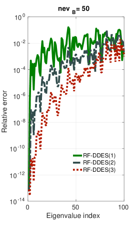
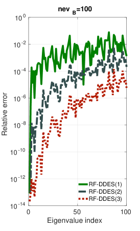
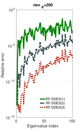
Fig. 3: Relative errors of the approximation of the lowest $nev=100$ eigenvalues for the “qa8fk/qafm” matrix pencil. Left: $nev_{B}=50$. Center: $nev_{B}=100$. Right: $nev_{B}=200$.

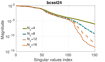
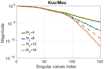
Fig. 4: The 150 leading singular values of $\Re e\left\{\sum_{\ell=1}^{N_{c}}\omega_{\ell}S_{\zeta_{\ell}}^{-1}\right\}$ for matrix pencils “bcsst24” and “Kuu/Muu”.

Table 3: Number of iterations performed by Algorithm 3.1 for the matrix pencils listed in Table 1. ’$s$’ denotes the number of interface variables.

Mat. pencil	$s$	$s/n$	$N_{c}=2$	$N_{c}=4$	$N_{c}=8$	$N_{c}=12$	$N_{c}=16$
bcsst24	449	0.12	164	133	111	106	104
Kuu/Muu	720	0.10	116	74	66	66	66
FDmesh1	300	0.01	58	40	36	35	34
bcsst39	475	0.01	139	93	75	73	72
qa8fk/qa8fm	1272	0.01	221	132	89	86	86

Table 3 lists the number of iterations performed by Algorithm 3.1 as the value of $N_{c}$ increases. Observe that for matrix pencils 2), 3), 4) and 5) this number can be less than $nev$ (recall the “early termination” property discussed in Proposition 1), even for values of $N_{c}$ as low as $N_{c}=2$. Moreover, Figure 4 plots the 150 leading singular values of matrix $\Re e\left\{\sum_{\ell=1}^{N_{c}}\omega_{\ell}S(\zeta_{\ell})^{-1}\right\}$ for matrix pencils “bcsst24” and “Kuu/Muu” as $N_{c}=4,\ 8,\ 12$ and $N_{c}=16$. In agreement with the discussion in Section 3.2, the magnitude of the trailing $s-{\rm rank}\left(\left[y^{(1)},\ldots,y^{(nev)}\right]\right)$ singular values approaches zero as the value of $N_{c}$ increases.

Except the value of $N_{c}$, the number of subdomains $p$ might also affect the number of iterations performed by Algorithm 3.1. Figure 5 shows the total number of iterations performed by Algorithm 3.1 when applied to matrix “FDmesh1” for $p=2,\ 4,\ 8$ and $p=16$ subdomains. For each different value of $p$ we considered $N_{c}=2,\ 4,\ 8,\ 12$, and $N_{c}=16$ quadrature nodes. The interval $[\alpha,\beta]$ was set so that it included only eigenvalues $\lambda_{1},\ldots,\lambda_{200}$ ($nev=200$). Observe that higher values of $p$ might lead to an increase in the number of iterations performed by Algorithm 3.1. For example, when the number of subdomains is set to $p=2$ or $p=4$, setting $N_{c}=2$ is sufficient for Algorithm 3.1 to terminate in less than $nev$ iterations On the other hand, when $p\geq 8$, we need at least $N_{c}\geq 4$ if a similar number of iterations is to be performed.

Fig. 5: Total number of iterations performed by Algorithm 3.1 when applied to matrix “FDmesh1” (where $[\alpha,\beta]=[\lambda_{1},\lambda_{200}]$). Results reported are for all different combinations of $p=2,\ 4,\ 8$ and $p=16$, and $N_{c}=1,\ 2,\ 4,\ 8$ and $N_{c}=16$.

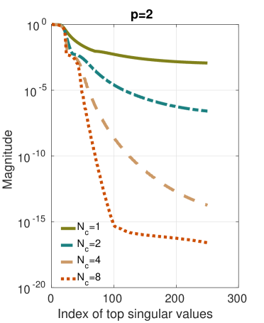
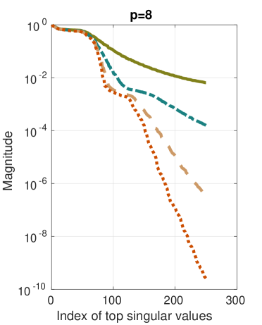
Fig. 6: The leading $250$ singular values of $\Re e\left\{\sum_{\ell=1}^{N_{c}}\omega_{\ell}S(\zeta_{\ell})^{-1}\right\}$ for the same problem as in Figure 5. Left: $p=2$. Right: $p=8$. For both values of $p$ we set $N_{c}=1,\ 2,\ 4,$ and $N_{c}=8$.

This potential increase in the number of iterations performed by Algorithm 3.1 for larger values of $p$ is a consequence of the fact that the columns of matrix $Y=\left[y^{(1)},\ldots,y^{(nev)}\right]$ now lie in a higher-dimensional subspace. This might not only increase the rank of $Y$, but also affect the decay of the singular values of $\Re e\left\{\sum_{\ell=1}^{N_{c}}\omega_{\ell}S(\zeta_{\ell})^{-1}\right\}$. This can be seen more clearly in Figure 6 where we plot the leading $250$ singular values of $\Re e\left\{\sum_{\ell=1}^{N_{c}}\omega_{\ell}S(\zeta_{\ell})^{-1}\right\}$ of the problem in Figure 5 for two different values of $p$, $p=2$ and $p=8$. Note that the leading singular values decay more slowly for the case $p=8$. Similar results were observed for different values of $p$ and for all matrix pencils listed in Table 1.

6.3 A comparison of RF-DDES and RF-KRYLOV in distributed computing environments

In this section we compare the performance of RF-KRYLOV and RF-DDES on distributed computing environments for the matrices listed in Table 4. All eigenvalue problems in this section are of the form $(A,I)$, i.e., standard eigenvalue problems. Matrices “boneS01” and “shipsec8” can be found in the SuiteSparse matrix collection. Similarly to “FDmesh1”, matrices “FDmesh2” and “FDmesh3” were generated by a Finite Differences discretization of the Laplacian operator on the unit plane using Dirichlet boundary conditions and two different mesh sizes so that $n=250,000$ (“FDmesh2”) and $n=1,000,000$ (“FDmesh3”).

Table 4: $n$: size of $A$, $nnz(A)$: number of non-zero entries in matrix $A$. $s_{2}$ and $s_{4}$ denote the number of interface variables when $p=2$ and $p=4$, respectively.

#	Matrix	$n$	$nnz(A)/n$	$s_{2}$	$s_{4}$	$[\lambda_{1},\lambda_{101},\lambda_{201},\lambda_{300}]$
1.	shipsec8	114,919	28.74	4,534	9,001	[3.2e-2, 1.14e-1, 1.57e-2, 0.20]
2.	boneS01	172,224	32.03	10,018	20,451	[2.8e-3, 24.60, 45.42, 64.43]
3.	FDmesh2	250,000	4.99	1,098	2,218	[7.8e-5, 5.7e-3, 1.08e-2, 1.6e-2]
4.	FDmesh3	1,000,000	4.99	2,196	4,407	[1.97e-5, 1.4e-3, 2.7e-3, 4.0e-3]

Throughout the rest of this section we will keep $N_{c}=2$ fixed, since this option was found the best both for RF-KRYLOV and RF-DDES.

6.3.1 Wall-clock time comparisons

We now consider the wall-clock times achieved by RF-KRYLOV and RF-DDES when executing both schemes on $\tau=2,\ 4,\ 8,\ 16$ and $\tau=32$ compute cores. For RF-KRYLOV, the value of $\tau$ will denote the number of single-threaded MPI processes. For RF-DDES, the number of MPI processes will be equal to the number of subdomains, $p$, and each MPI process will utilize $\tau/p$ compute threads. Unless mentioned otherwise, we will assume that RF-DDES is executed with $\psi=3$ and $nev_{B}=100$.

Table 5: Number of iterations performed by RF-KRYLOV (denoted as RFK) and Algorithm 3.1 in RF-DDES (denoted by RFD(2) and RFD(4), with the number inside the parentheses denoting the value of $p$) for the matrix pencils listed in Table 4. The convergence criterion in both RF-KRYLOV and Algorithm 3.1 was tested every ten iterations.

		$nev=100$				$nev=200$				$nev=300$
		RFK	RFD($2$)	RFD($4$)		RFK	RFD($2$)	RFD($4$)		RFK	RFD($2$)	RFD($4$)
shipsec8		280	170	180		500	180	280		720	190	290
boneS01		240	350	410		480	520	600		620	640	740
FDmesh2		200	100	170		450	130	230		680	160	270
FDmesh3		280	150	230		460	180	290		690	200	380

0.4 $nev=100$ $nev=200$ $nev=300$ $nev_{B}$ $25$ $50$ $100$ $25$ $50$ $100$ $25$ $50$ $100$ shipsec8 1.4e-3 2.2e-5 2.4e-6 3.4e-3 1.9e-3 1.3e-5 4.2e-3 1.9e-3 5.6e-4 boneS01 5.2e-3 7.1e-4 2.2e-4 3.8e-3 5.9e-4 4.1e-4 3.4e-3 9.1e-4 5.1e-4 FDmesh2 4.0e-5 2.5e-6 1.9e-7 3.5e-4 9.6e-5 2.6e-6 3.2e-4 2.0e-4 2.6e-5 FDmesh3 6.2e-5 8.5e-6 4.3e-6 6.3e-4 1.1e-4 3.1e-5 9.1e-4 5.3e-4 5.3e-5

Table 6: Maximum relative error of the approximate eigenvalues returned by RF-DDES for the matrix pencils listed in Table 4.

0.7 $nev=100$ $nev=200$ $nev=300$ Matrix RFK RFD($2$) RFD($4$) RFK RFD($2$) RFD($4$) RFK RFD($2$) RFD($4$) shipsec8($\tau=2$) 114 195 - 195 207 - 279 213 -  shipsec8($\tau=4$) 76 129 93 123 133 103 168 139 107  shipsec8($\tau=8$) 65 74 56 90 75 62 127 79 68  shipsec8($\tau=16$) 40 51 36 66 55 41 92 57 45  shipsec8($\tau=32$) 40 36 28 62 41 30 75 43 34 boneS01($\tau=2$) 94 292 - 194 356 - 260 424 -  boneS01($\tau=4$) 68 182 162 131 230 213 179 277 260  boneS01($\tau=8$) 49 115 113 94 148 152 121 180 187  boneS01($\tau=16$) 44 86 82 80 112 109 93 137 132  boneS01($\tau=32$) 51 66 60 74 86 71 89 105 79 FDmesh2($\tau=2$) 241 85 - 480 99 - 731 116 -  FDmesh2($\tau=4$) 159 34 63 305 37 78 473 43 85  FDmesh2($\tau=8$) 126 22 23 228 24 27 358 27 31  FDmesh2($\tau=16$) 89 16 15 171 17 18 256 20 21  FDmesh2($\tau=32$) 51 12 12 94 13 14 138 15 20 FDmesh3($\tau=2$) 1021 446 - 2062 502 - 3328 564 -  FDmesh3($\tau=4$) 718 201 281 1281 217 338 1844 237 362  FDmesh3($\tau=8$) 423 119 111 825 132 126 1250 143 141  FDmesh3($\tau=16$) 355 70 66 684 77 81 1038 88 93  FDmesh3($\tau=32$) 177 47 49 343 51 58 706 62 82

Table 7: Wall-clock times of RF-KRYLOV and RF-DDES using $\tau=2,\ 4,\ 8,\ 16$ and $\tau=32$ computational cores. RFD(2) and RFD(4) denote RF-DDES with $p=2$ and $p=4$ subdomains, respectively.

Table 7 lists the wall-clock time required by RF-KRYLOV and RF-DDES to approximate the $nev=100,\ 200$ and $nev=300$ algebraically smallest eigenvalues of the matrices listed in Table 4. For RF-DDES we considered two different values of $p$; $p=2$ and $p=4$. Overall, RF-DDES was found to be faster than RF-KRYLOV, with an increasing performance gap for higher values of $nev$. Table 5 lists the number of iterations performed by RF-KRYLOV and Algorithm 3.1 in RF-DDES. For all matrices but “boneS01”, Algorithm 3.1 required fewer iterations than RF-KRYLOV. Table 6 lists the maximum relative error of the approximate eigenvalues returned by RF-DDES when $p=4$. The decrease in the accuracy of RF-DDES as $nev$ increases is due the fact that $nev_{B}$ remains bounded. Typically, an increase in the value of $nev$ should be also accompanied by an increase in the value of $nev_{B}$, if the same level of maximum relative error need be retained. On the other hand, RF-KRYLOV always computed all $nev$ eigenpairs up to the maximum attainable accuracy.

0.7 $nev=100$ $nev=200$ $nev=300$ Matrix RFK RFD($2$) RFD($4$) RFK RFD($2$) RFD($4$) RFK RFD($2$) RFD($4$) shipsec8($\tau=2$) 104 153 - 166 155 - 222 157 -  shipsec8($\tau=4$) 71 93 75 107 96 80 137 96 82  shipsec8($\tau=8$) 62 49 43 82 50 45 110 51 47  shipsec8($\tau=16$) 38 32 26 61 33 28 83 34 20  shipsec8($\tau=32$) 39 21 19 59 23 20 68 24 22 boneS01($\tau=2$) 86 219 - 172 256 - 202 291 -  boneS01($\tau=4$) 64 125 128 119 152 168 150 178 199  boneS01($\tau=8$) 46 77 88 84 95 117 104 112 140  boneS01($\tau=16$) 43 56 62 75 70 85 86 84 102  boneS01($\tau=32$) 50 42 44 72 51 60 82 63 61 FDmesh2($\tau=2$) 227 52 - 432 59 - 631 65 -  FDmesh2($\tau=4$) 152 22 36 287 24 42 426 26 45  FDmesh2($\tau=8$) 122 13 14 215 14 16 335 15 18  FDmesh2($\tau=16$) 85 9 8 164 10 10 242 11 11  FDmesh2($\tau=32$) 50 6 6 90 7 8 127 8 10 FDmesh3($\tau=2$) 960 320 - 1817 341 - 2717 359 -  FDmesh3($\tau=4$) 684 158 174 1162 164 192 1582 170 201  FDmesh3($\tau=8$) 406 88 76 764 91 82 1114 94 88  FDmesh3($\tau=16$) 347 45 43 656 48 49 976 51 52  FDmesh3($\tau=32$) 173 28 26 328 28 32 674 31 41

Table 8: Time elapsed to apply to apply the rational filter in RF-KRYLOV and RF-DDES using $\tau=2,\ 4,\ 8,\ 16$ and $\tau=32$ compute cores. RFD(2) and RFD(4) denote RF-DDES with $p=2$ and $p=4$ subdomains, respectively. For RF-KRYLOV the times listed also include the amount of time spent on factorizing matrices $A-\zeta_{\ell}M,\ \ell=1,\ldots,N_{c}$. For RF-DDES, the times listed also include the amount of time spent in forming and factorizing matrices $S_{\zeta_{\ell}},\ \ell=1,\ldots,N_{c}$.

Table 8 lists the amount of time spent on the triangular substitutions required to apply the rational filter in RF-KRYLOV, as well as the amount of time spent on forming and factorizing the Schur complement matrices and applying the rational filter in RF-DDES. For the values of $nev$ tested in this section, these procedures were found to be the computationally most expensive ones.

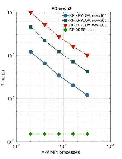
(a) FDmesh2 ($n=250,000$).

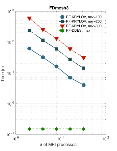
(b) FDmesh3 ($n=1,000,000$).

Fig. 7: Time spent on orthonormalization in RF-KRYLOV and RF-DDES when computing the $nev=100,\ 200$ and $nev=300$ algebraically smallest eigenvalues and associated eigenvectors of matrices “FDmesh2” and “FDmesh3”.

Figure 7 plots the total amount of time spent on orthonormalization by RF-KRYLOV and RF-DDES when applied to matrices “FDmesh2” and “FDmesh3”. For RF-KRYLOV, we report results for all different values of $nev$ and number of MPI processes. For RF-DDES we only report the highest times across all different values of $nev,\ \tau$ and $p$. RF-DDES was found to spend a considerably smaller amount of time on orthonormalization than what RF-KRYLOV did, mainly because $s$ was much smaller than $n$ (the values of $s$ for $p=2$ and $p=4$ can be found in Table 4). Indeed, if both RF-KRYLOV and Algorithm 3.1 in RF-DDES perform a similar number of iterations, we expect the former to spend roughly $n/s$ more time on orthonormalization compared to RF-DDES.

Fig. 8: Amount of time required to apply the rational filter (“Interface”), form the subspace associated with the interior variables (“Interior”), and total wall-clock time (“Total”) obtained by an MPI-only execution of RF-DDES for the case where $nev=300$. Left: “shipsec8”. Right: “FDmesh2”.

Figure 8 lists the wall-clock times achieved by an MPI-only implementation of RF-DDES, i.e., $p$ still denotes the number of subdomains but each subdomain is handled by a separate (single-threaded) MPI process, for matrices “shipsec8” and “FDmesh2”. In all cases, the MPI-only implementation of RF-DDES led to higher wall-clock times than those achieved by the hybrid implementations discussed in Tables 7 and 8. More specifically, while the MPI-only implementation reduced the cost to construct and factorize the distributed $S_{\zeta_{\ell}}$ matrices, the application of the rational filter in Algorithm 3.1 became more expensive due to: a) each linear system solution with $S_{\zeta_{\ell}}$ required more time, b) a larger number of iterations had to be performed as $p$ increased (Algorithm 3.1 required 190, 290, 300, 340 and 370 iterations for “shipsec8”, and 160, 270, 320, 350, and 410 iterations for “FDmesh2” as $p=2,\ 4,\ 8,\ 16$ and $p=32$, respectively). One more observation is that for the MPI-only version of RF-DDES, its scalability for increasing values of $p$ is limited by the scalability of the linear system solver which is typically not high. This suggests that reducing $p$ and applying RF-DDES recursively to the local pencils $(B_{\sigma}^{(j)},M_{B}^{(j)}),\ j=1,\ldots,p$ might be the best combination when only distributed memory parallelism is considered.

7 Conclusion

In this paper we proposed a rational filtering domain decomposition approach (termed as RF-DDES) for the computation of all eigenpairs of real symmetric pencils inside a given interval $[\alpha,\beta]$. In contrast with rational filtering Krylov approaches, RF-DDES applies the rational filter only to the interface variables. This has several advantages. First, orthogonalization is performed on vectors whose length is equal to the number of interface variables only. Second, the Krylov projection method may converge in fewer than $nev$ iterations. Third, it is possible to solve the original eigenvalue problem associated with the interior variables in real arithmetic and with trivial parallelism with respect to each subdomain. RF-DDES can be considerably faster than rational filtering Krylov approaches, especially when a large number of eigenvalues is located inside $[\alpha,\beta]$.

In future work, we aim to extend RF-DDES by taking advantage of additional levels of parallelism. In addition to the ability to divide the initial interval $[\alpha,\beta]$ into non-overlapping subintervals and process them in parallel, e.g. see [24, 21], we can also assign linear system solutions associated with different quadrature nodes to different groups of processors. Another interesting direction is to consider the use of iterative solvers to solve the linear systems associated with $S(\zeta_{1}),\ldots,S(\zeta_{N_{c}})$. This could be helpful when RF-DDES is applied to the solution of symmetric eigenvalue problems arising from 3D domains. On the algorithmic side, it would be of interest to develop more efficient criteria to set the value of $nev_{B}^{(j)},\ j=1,\ldots,p$ in each subdomain, perhaps by adapting the work in [38]. In a similar context, it would be interesting to also explore recursive implementations of RF-DDES. For example, RF-DDES could be applied individually to each matrix pencil $(B_{\sigma}^{(j)},M_{B}^{(j)}),\ j=1,\ldots,p$ to compute the $nev_{B}^{(j)}$ eigenvectors of interest. This could be particularly helpful when either $d_{j}$, the number of interior variables of the $j$th subdomain, or $nev_{B}^{(j)}$, are large.

8 Acknowledgments

Vassilis Kalantzis was partially supported by a Gerondelis Foundation Fellowship. The authors acknowledge the Minnesota Supercomputing Institute (MSI; http://www.msi.umn.edu) at the University of Minnesota for providing resources that contributed to the research results reported within this paper.

References

- [1] Intel Math Kernel Library. Reference Manual, Intel Corporation, 2009. Santa Clara, USA. ISBN 630813-054US.
- [2] M. Abramowitz, Handbook of Mathematical Functions, With Formulas, Graphs, and Mathematical Tables,, Dover Publications, Incorporated, 1974.
- [3] P. R. Amestoy, I. S. Duff, J.-Y. L’Excellent, and J. Koster, A fully asynchronous multifrontal solver using distributed dynamic scheduling, SIAM Journal on Matrix Analysis and Applications, 23 (2001), pp. 15–41.
- [4] A. L. S. Andrew V. Knyazev, Preconditioned gradient-type iterative methods in a subspace for partial generalized symmetric eigenvalue problems, SIAM Journal on Numerical Analysis, 31 (1994), pp. 1226–1239.
- [5] A. P. Austin and L. N. Trefethen, Computing eigenvalues of real symmetric matrices with rational filters in real arithmetic, SIAM Journal on Scientific Computing, 37 (2015), pp. A1365–A1387.
- [6] S. Balay, W. D. Gropp, L. C. McInnes, and B. F. Smith, Efficient management of parallelism in object oriented numerical software libraries, in Modern Software Tools in Scientific Computing, E. Arge, A. M. Bruaset, and H. P. Langtangen, eds., Birkhäuser Press, 1997, pp. 163–202.
- [7] M. V. Barel, Designing rational filter functions for solving eigenvalue problems by contour integration, Linear Algebra and its Applications, (2015), pp. –.
- [8] M. V. Barel and P. Kravanja, Nonlinear eigenvalue problems and contour integrals, Journal of Computational and Applied Mathematics, 292 (2016), pp. 526 – 540.
- [9] C. Bekas and Y. Saad, Computation of smallest eigenvalues using spectral schur complements, SIAM J. Sci. Comput., 27 (2006), pp. 458–481.
- [10] J. K. Bennighof and R. B. Lehoucq, An automated multilevel substructuring method for eigenspace computation in linear elastodynamics, SIAM J. Sci. Comput., 25 (2004), pp. 2084–2106.
- [11] L. S. Blackford, J. Choi, A. Cleary, E. D’Azeuedo, J. Demmel, I. Dhillon, S. Hammarling, G. Henry, A. Petitet, K. Stanley, D. Walker, and R. C. Whaley, ScaLAPACK User’s Guide, Society for Industrial and Applied Mathematics, Philadelphia, PA, USA, 1997.
- [12] T. A. Davis and Y. Hu, The university of Florida sparse matrix collection, ACM Trans. Math. Softw., 38 (2011), pp. 1:1–1:25.
- [13] S. B. et al., PETSc users manual, Tech. Rep. ANL-95/11 - Revision 3.6, Argonne National Laboratory, 2015.
- [14] , PETSc Web page. http://www.mcs.anl.gov/petsc, 2015.
- [15] W. Gao, X. S. Li, C. Yang, and Z. Bai, An implementation and evaluation of the amls method for sparse eigenvalue problems, ACM Trans. Math. Softw., 34 (2008), pp. 20:1–20:28.
- [16] R. G. Grimes, J. G. Lewis, and H. D. Simon, A shifted block lanczos algorithm for solving sparse symmetric generalized eigenproblems, SIAM J. Matrix Anal. Appl., 15 (1994), pp. 228–272.
- [17] S. Güttel, E. Polizzi, P. T. P. Tang, and G. Viaud, Zolotarev quadrature rules and load balancing for the feast eigensolver, SIAM Journal on Scientific Computing, 37 (2015), pp. A2100–A2122.
- [18] V. Kalantzis, J. Kestyn, E. Polizzi, and Y. Saad, Domain decomposition approaches for accelerating contour integration eigenvalue solvers for symmetric eigenvalue problems, Preprint, Dept. Computer Science and Engineering, University of Minnesota, Minneapolis, MN, 2016, (2016).
- [19] V. Kalantzis, R. Li, and Y. Saad, Spectral schur complement techniques for symmetric eigenvalue problems, Electronic Transactions on Numerical Analysis, 45 (2016), pp. 305–329.
- [20] G. Karypis and V. Kumar, A fast and high quality multilevel scheme for partitioning irregular graphs, SIAM Journal on Scientific Computing, 20 (1998), pp. 359–392.
- [21] J. Kestyn, V. Kalantzis, E. Polizzi, and Y. Saad, Pfeast: A high performance sparse eigenvalue solver using distributed-memory linear solvers, in In Proceedings of the ACM/IEEE Supercomputing Conference (SC16), 2016.
- [22] J. Kestyn, E. Polizzi, and P. T. P. Tang, Feast eigensolver for non-hermitian problems, SIAM Journal on Scientific Computing, 38 (2016), pp. S772–S799.
- [23] L. Komzsik and T. Rose, Parallel methods on large-scale structural analysis and physics applications substructuring in msc/nastran for large scale parallel applications, Computing Systems in Engineering, 2 (1991), pp. 167 – 173.
- [24] R. Li, Y. Xi, E. Vecharynski, C. Yang, and Y. Saad, A thick-restart lanczos algorithm with polynomial filtering for hermitian eigenvalue problems, SIAM Journal on Scientific Computing, 38 (2016), pp. A2512–A2534.
- [25] S. Lui, Kron’s method for symmetric eigenvalue problems, Journal of Computational and Applied Mathematics, 98 (1998), pp. 35 – 48.
- [26] , Domain decomposition methods for eigenvalue problems, Journal of Computational and Applied Mathematics, 117 (2000), pp. 17 – 34.
- [27] F. Pellegrini, Scotch and libScotch 5.1 User’s Guide, INRIA Bordeaux Sud-Ouest, IPB & LaBRI, UMR CNRS 5800, 2010.
- [28] B. Philippe and Y. Saad, On correction equations and domain decomposition for computing invariant subspaces, Computer Methods in Applied Mechanics and Engineering, 196 (2007), pp. 1471 – 1483. Domain Decomposition Methods: recent advances and new challenges in engineering.
- [29] E. Polizzi, Density-matrix-based algorithm for solving eigenvalue problems, Phys. Rev. B, 79 (2009), p. 115112.
- [30] T. Sakurai and H. Sugiura, A projection method for generalized eigenvalue problems using numerical integration, Journal of Computational and Applied Mathematics, 159 (2003), pp. 119 – 128. 6th Japan-China Joint Seminar on Numerical Mathematics; In Search for the Frontier of Computational and Applied Mathematics toward the 21st Century.
- [31] H. D. Simon, The lanczos algorithm with partial reorthogonalization, Mathematics of Computation, 42 (1984), pp. 115–142.
- [32] B. F. Smith, P. E. Bjørstad, and W. D. Gropp, Domain Decomposition: Parallel Multilevel Methods for Elliptic Partial Differential Equations, Cambridge University Press, New York, NY, USA, 1996.
- [33] M. Snir, S. Otto, S. Huss-Lederman, D. Walker, and J. Dongarra, MPI-The Complete Reference, Volume 1: The MPI Core, MIT Press, Cambridge, MA, USA, 2nd. (revised) ed., 1998.
- [34] P. T. P. Tang and E. Polizzi, Feast as a subspace iteration eigensolver accelerated by approximate spectral projection, SIAM Journal on Matrix Analysis and Applications, 35 (2014), pp. 354–390.
- [35] A. Toselli and O. Widlund, Domain decomposition methods: algorithms and theory, vol. 3, Springer, 2005.
- [36] J. Winkelmann and E. Di Napoli, Non-linear least-squares optimization of rational filters for the solution of interior eigenvalue problems, arXiv preprint arXiv:1704.03255, (2017).
- [37] Y. Xi and Y. Saad, Computing partial spectra with least-squares rational filters, SIAM Journal on Scientific Computing, 38 (2016), pp. A3020–A3045.
- [38] C. Yang, W. Gao, Z. Bai, X. S. Li, L.-Q. Lee, P. Husbands, and E. Ng, An algebraic substructuring method for large-scale eigenvalue calculation, SIAM Journal on Scientific Computing, 27 (2005), pp. 873–892.