Controlling Physical Attributes in GAN-Accelerated Simulation of Electromagnetic Calorimeters
Abstract
High-precision modeling of subatomic particle interactions is critical for many fields within the physical sciences, such as nuclear physics and high energy particle physics. Most simulation pipelines in the sciences are computationally intensive – in a variety of scientific fields, Generative Adversarial Networks have been suggested as a solution to speed up the forward component of simulation, with promising results. An important component of any simulation system for the sciences is the ability to condition on any number of physically meaningful latent characteristics that can effect the forward generation procedure. We introduce an auxiliary task to the training of a Generative Adversarial Network on particle showers in a multi-layer electromagnetic calorimeter, which allows our model to learn an attribute-aware conditioning mechanism.
1 Introduction
Modeling the interactions of particles with media is critical across many many physical sciences. Detailed simulation of particle collisions and subsequent interactions at the LHC experiments, along with simulating exact detector response, is very computationally expensive, requiring billions of CPU hours and roughly half of LHC computing resources [1, 2, 3].
Recently, deep learning-based generative models including Generative Adversarial Networks [4] and Variational Auto-Encoders [5] have been proposed and tested as a solution to significantly speed up scientific simulation in Oncology [6], Cosmology [7, 8, 9], and High Energy Physics [10, 11], and many other basic science fields. We propose a simple extension to the CaloGAN model [10] allowing such a generation model to be conditioned on a vector of physically meaningful characteristics. We introduce a series of auxiliary tasks to encourage our model to learn , where is a vector of meaningful characteristics which should guide the generation procedure.
2 The Dataset
The publicly available dataset from Ref. [12], composed of 500,000 , 500,000 , and 400,000 Geant4-generated showers, is used to construct and validate a proposed architecture for conditional modeling. The detector geometry present in the data consists of a cubic region along the direction of mm3 of an ATLAS-inspired EM calorimeter, at a distance of mm from (0,0,0). The volume is radially segmented into three layers of depth 90 mm, 347 mm, and 43 mm composed of alternating layers of lead and liquid Argon.
In this work, all Geant4 coordinates native to the simulation are transformed into ATLAS coordinates for consistency with practical use-cases in experiments.
3 Generative Adversarial Networks
Generative Adversarial Networks (GAN) [4] are a method to learna generative model by recasting the generation procedure as a minimax game between two actors that are parameterized by deep neural networks. A generator network is tasked with building samples that are very similar to some target data distribution, and a discriminator network (the adversary) is tasked with learning to distinguish real-looking samples from fake-looking samples.
Formally, assume we have a data distribution we wish to model, . We construct a generator network that maps a -dimensional latent prior to synthetic samples . The map implicitly defines a learned probability distribution from which we can sample, . In order to direct towards the data distribution , a discriminator network is tasked with taking a sample and classifying it with a label as originating from the data distribution () or from the implicit synthetic distribution (), i.e., .
In the original formulation of GANs [4] a loss is constructed (Eqn. 1) to guide the learning towards towards equilibrium. When and are allowed to be drawn from the space of all continuous functions (i.e., they have infinite capacity), this system converges to a unique Nash Equilibrium [13] in which the implicit distribution exactly recovers the target data distribution , and is everywhere [4]. It can be shown [4] that this procedure minimizes the Jensen-Shannon divergence between and , .
| (1) |
In the original formulation, minimizes while minimizes , i.e., the game is zero sum. However, this formulation suffers from gradient saturation when a synthetic sample is seen as very fake, i.e., when , stagnating the learning procedure due to near-zero gradients. To overcome this, Ref. [4] proposes the non-saturating heuristic, replacing the generator objective with Eq. 2, which it minimizes just as before. This formulation is utilized in our experiments, and we let represent the same quantity as in Eq. 1, except now it is only used for the discriminator.
| (2) |
Through architecture design [14, 15, 16, 17, 18, 19] and more theoretically-sound training objectives used [20, 21, 22, 23, 24, 25, 26], GANs have emerged as one of the most promising methods for neural networks to learn generative models of complicated and structured data spaces. We follow Ref. [27] and impose task-specific metrics which allow us to move away from likelihood-level notions of quality which do not directly translate to tasks of interest. We utilize the original heuristic loss formulation (Eq. 2) with label flipping [19] in lieu of mroe recent advances. The authors expect future work will experiment with effective conditioning mechanisms for other more popular GAN formulations such as the Wasserstein GAN [21] and the Cramér GAN [26].
4 The Conditional CaloGAN
To create a GAN based simulator that presents a useful solution for fast simulation, we need not only learn , but we must also approximate , where is a vector of conditioning attributes. Given the dataset outlined in Sec. 2, is chosen to be , where and are the incident coordinates and and are incident angles. As per Ref. [10], an absolute-deviance is defined over requested and reconstructed energy from a simulated collision, encouraging the GAN to learn the conditional distribution. In this work, a generalization is presented. For quantities that do not have a direct mathematical formula given a shower (i.e., , and ), we build a separate head on the discriminator to learn a specific submodel which focuses on learning to regress on said quantities given a shower as input. This estimate is learned along with the normal alternating gradient step. To both and from Sec. 3, (Eq. 3) is added such that both players seek to minimize the attribute reconstruction error.
| (3) |
Note that in Eq. 3 a hyperparameter is included to allow us to individually control the contribution for each attribute reconstruction task. Combining this with the energy conditioning loss and associated weight from the original CaloGAN formulation [10], our final optimization problem consists of the generator minimizing and the discriminator minimizing .
5 Sparsity Considerations
As in most scientific applications, sparsity plays an important role in determining how viable a generates sample is. In the original CaloGAN work [10], a raw sparsity (or occupancy) calculation is performed and fed as additional information to the discriminator. For an image , the sparsity is calculated as:
| (4) |
Note that although this allows the discriminator to learn to reject generated samples that do not match the sparsity levels of real samples, this formulation does not allow for any gradient signal to propagate to the generator due to all-zero sub-derivatives of the indicator function . To ameliorate this deficiency, soft sparsity is introduced – a quantity that in the limit of tunable hyperparameters, converges to Eqn. 4. In particular, we define this quantity as
| (5) |
where , all matrix powers and operators are assumed to act pointwise on , and is the entry-wise 1-norm rather than the induced norm.
Examining Eqn. 5, we note that , and that the limit behavior for Eqn. 5 is consistent with Eqn. 4, i.e.,
| (6) |
This information is added to the discriminator in raw form as well as a minibatch discrimination [19] step in order to allow our model to learn the correct distribution of sparsity.
6 Experiment & Results
6.1 Setup
A Conditional CaloGAN (Sec. 4) with soft sparsity information (Sec. 5) is trained on the dataset described in Section 2. We perform our experiments on the simulated showers.
To allow the model to learn to generate translation invariant samples, we replace all locally connected layers in the original CaloGAN formulation with normal convolution layers, as well as a fully-convolutional attention mechanism to mediate layer-to-layer dependence. In addition, convolutional kernels are added as blurring operations to specific detector layers for smearing effects, where weights are initialized to for an filter and are not updated during training, which was empirically found to improve generation quality. This explicit blur operation allows the model to learn a factored problem which marginalizes out smearing effects, and allows the model to focus on important factors in shower patterns.
6.2 Results
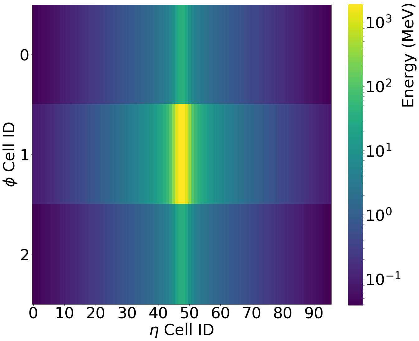
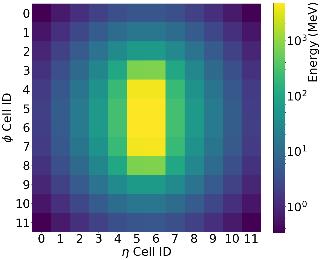
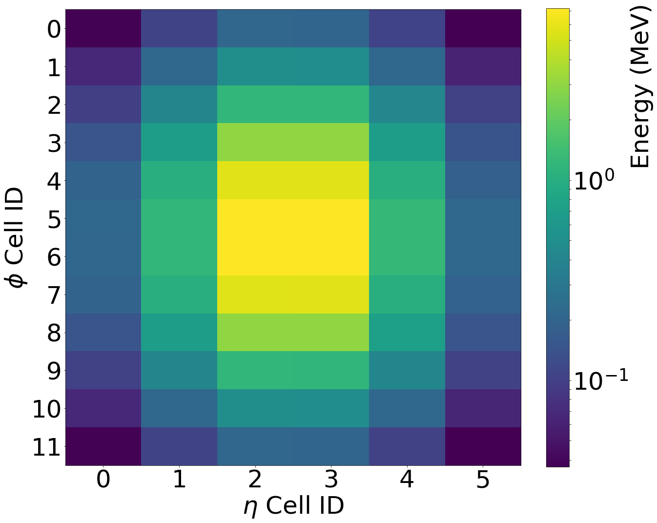
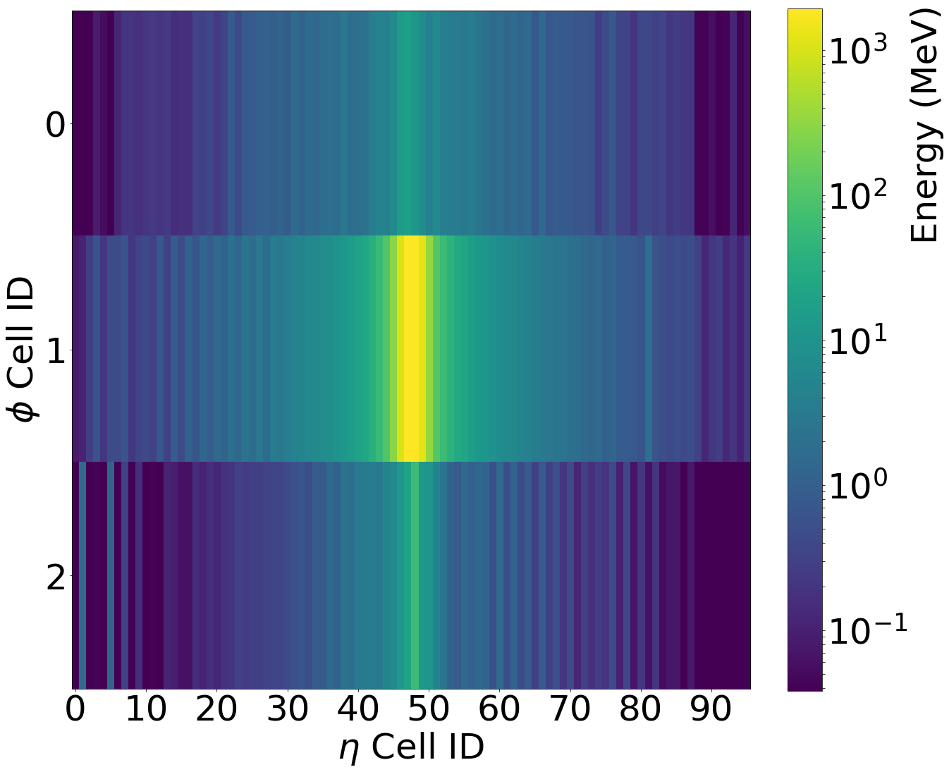
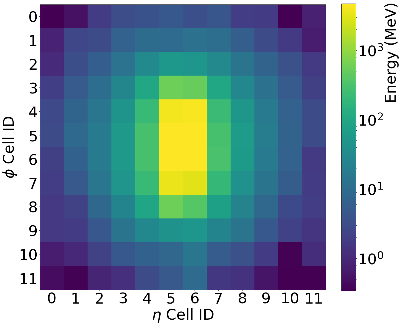
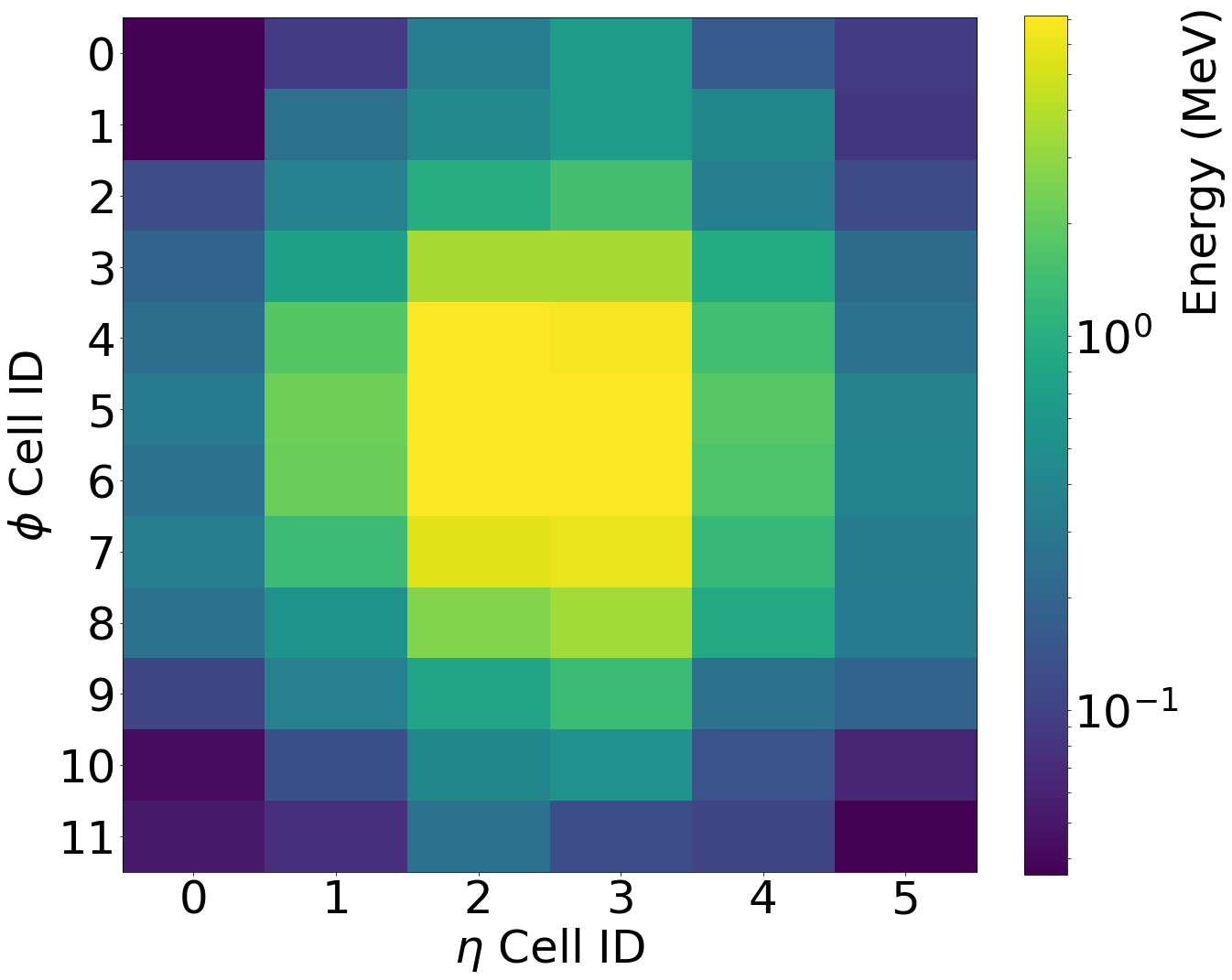
As a first layer of validation, and commensurate with the validation performed in Ref. [10], average images per calorimeter layer between images from the dataset of Geant4 images are compared to images generated from the proposed model, as shown in Figure 1. This visualization illustrates the increased energy dispersion compared to the original dataset presented in Ref. [10]. The comparison in Figure 1 shows a high level of visual agreement between GAN-generated and Geant4-generated showers.
In addition to aggregate image pattern validation, nearest GAN neighbors111By standard vectoral 2-norm. are retrieved for seven Geant4 images and used to validate that (a) our model does not memorize shower patterns, and (b) that the full space of displacements (both angular and positional) are explored.
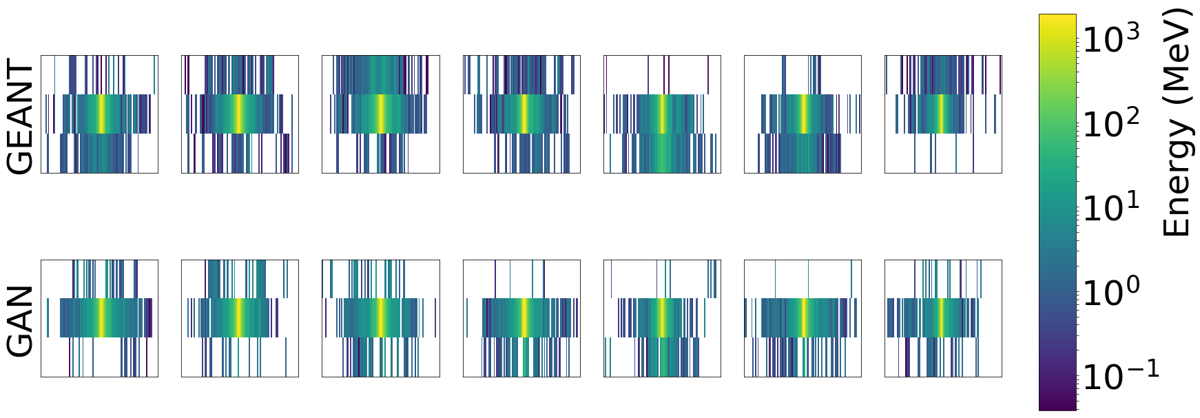
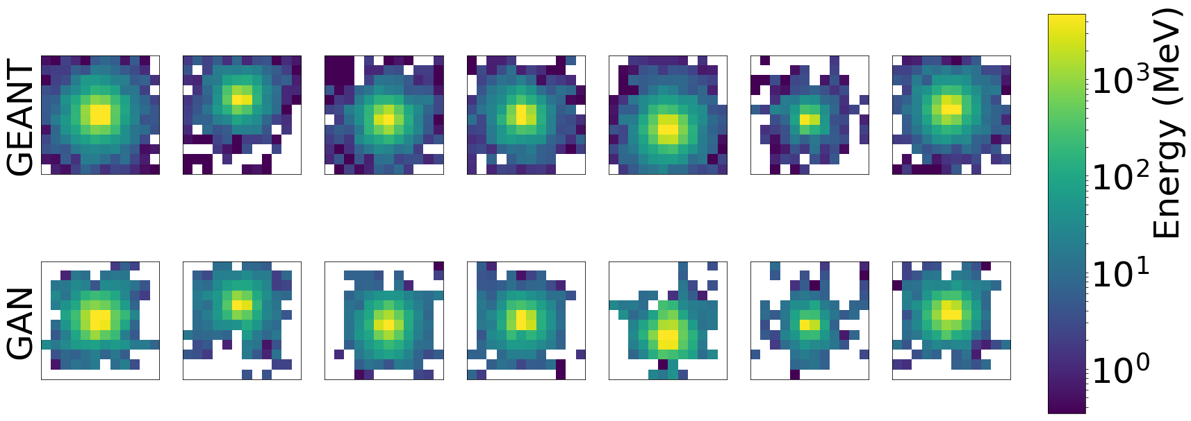
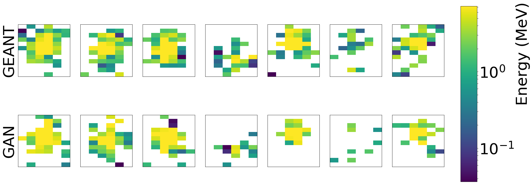
At the nearest-neighbor level, the model produces convincing energy deposition patterns, as shown in Figure 2. The model does not appear to memorize the training dataset. In addition, positional variance (observed by noticing energy centroid deviations from the center of the calorimeter image) is well explored by the GAN, as shown by GAN-generated images matching all positions given by Geant4.
To further verify our models ability to condition on physical attributes, the latent space for each conditioning variable is traversed, showing how the model learns about each conditioning factor. In any practical setting, such conditioning mechanisms will need to be tuned to a high level of fidelity.
To illustrate the model’s internal representation, incident energy, , and manifolds are traversed at regular intervals along the trained range. In Figure 3, incident energy is traversed, clearly showing more energetic behavior as the incident energy is increased from left to right.

Similarly, the latent space for is traversed, and the resulting impact on generated image is shown in Figure 4. We note that as increases, shower position shifts downward, which is consistent with the ATLAS coordinates used in the dataset described in Sec. 2.

Finally, as we traverse (Fig. 5) we illustrate the shower behavior dynamic using a difference between the middle point in interpolation space and each point along the traversal. As increases, we note that the width and dispersion decreases and the showers become significantly more centralized222In Figure 5, areas turning blue indicate that less energy is deposited in that particular section of the image at a given point in latent space., which is consistent with the ATLAS definition of .

7 Conclusion
In this work, we explore the ability of GANs to be conditioned on physically meaningful attributes towards the ultimate goal of creating a viable, comprehensive solution for fast, high fidelity simulation of electromagnetic calorimeters. Clearly, GANs show great potential for controllability of generation procedures, but much future work remains. In particular, a thorough investigation around dynamics between the attribute estimation portion of the network, , and the overall training objective should be pursued, particularly as it relates to the final fidelity of the attribute estimates. In addition, future work should examine newer GAN formulations (as outlined in Sec. 3) and their ability to improve image quality.
References
- [1] Flynn J 2015 Computing Resources Scrutiny Group Report Tech. Rep. CERN-RRB-2015-014 CERN Geneva URL https://cds.cern.ch/record/2002240
- [2] Karavakis E, Andreeva J, Campana S, Gayazov S, Jezequel S, Saiz P, Sargsyan L, Schovancova J, Ueda I and the Atlas Collaboration 2014 Journal of Physics: Conference Series 513 062024 URL http://stacks.iop.org/1742-6596/513/i=6/a=062024
- [3] Bozzi C 2015 LHCb Computing Resource usage in 2014 (II) Tech. Rep. LHCb-PUB-2015-004. CERN-LHCb-PUB-2015-004 CERN Geneva URL https://cds.cern.ch/record/1984010
- [4] Goodfellow I J, Pouget-Abadie J, Mirza M, Xu B, Warde-Farley D, Ozair S, Courville A and Bengio Y 2014 ArXiv e-prints (Preprint 1406.2661)
- [5] Kingma D P and Welling M 2013 ArXiv e-prints (Preprint 1312.6114)
- [6] Kadurin A, Aliper A, Kazennov A, Mamoshina P, Vanhaelen Q, Khrabrov K and Zhavoronkov A 2016 Oncotarget 8 ISSN 1949-2553
- [7] Ravanbakhsh S, Lanusse F, Mandelbaum R, Schneider J and Poczos B 2016 (Preprint 1609.05796)
- [8] Schawinski K, Zhang C, Zhang H, Fowler L and Santhanam G K 2017 Monthly Notices of the Royal Astronomical Society 467 L110–L114 (Preprint 1702.00403)
- [9] Mustafa M, Bard D, Bhimji W, Al-Rfou R and Lukić Z 2017 ArXiv e-prints (Preprint 1706.02390)
- [10] Paganini M, de Oliveira L and Nachman B 2017 (Preprint 1705.02355)
- [11] de Oliveira L, Paganini M and Nachman B 2017 Computing and Software for Big Science 1 4 ISSN 2510-2044 URL https://doi.org/10.1007/s41781-017-0004-6
- [12] Paganini M, de Oliveira L and Nachman B 2017 Electromagnetic calorimeter shower images with variable incidence angle and position URL http://dx.doi.org/10.17632/5fnxs6b557.2
- [13] Goodfellow I J 2017 CoRR abs/1701.00160 URL http://arxiv.org/abs/1701.00160
- [14] Radford A, Metz L and Chintala S 2015 ArXiv e-prints (Preprint 1511.06434) URL http://arxiv.org/abs/1511.06434
- [15] Reed S E, Akata Z, Mohan S, Tenka S, Schiele B and Lee H 2016 ArXiv e-prints (Preprint 1610.02454) URL http://arxiv.org/abs/1610.02454
- [16] Odena A, Olah C and Shlens J 2016 ArXiv e-prints (Preprint 1610.09585)
- [17] Zhang H, Xu T, Li H, Zhang S, Huang X, Wang X and Metaxas D 2016 ArXiv e-prints (Preprint 1612.03242)
- [18] Mirza M and Osindero S 2014 ArXiv e-prints (Preprint 1411.1784) URL http://arxiv.org/abs/1411.1784
- [19] Salimans T, Goodfellow I J, Zaremba W, Cheung V, Radford A and Chen X 2016 ArXiv e-prints (Preprint 1606.03498) URL http://arxiv.org/abs/1606.03498
- [20] Chen X, Duan Y, Houthooft R, Schulman J, Sutskever I and Abbeel P 2016 ArXiv e-prints (Preprint 1606.03657) URL http://arxiv.org/abs/1606.03657
- [21] Arjovsky M, Chintala S and Bottou L 2017 ArXiv e-prints (Preprint 1701.07875)
- [22] Gulrajani I, Ahmed F, Arjovsky M, Dumoulin V and Courville A 2017 ArXiv e-prints (Preprint 1704.00028)
- [23] Qi G 2017 CoRR abs/1701.06264 URL http://arxiv.org/abs/1701.06264
- [24] Nowozin S, Cseke B and Tomioka R 2016 ArXiv e-prints (Preprint 1606.00709)
- [25] Lin M 2017 ArXiv e-prints (Preprint 1704.06191)
- [26] Bellemare M G, Danihelka I, Dabney W, Mohamed S, Lakshminarayanan B, Hoyer S and Munos R 2017 CoRR abs/1705.10743 URL http://arxiv.org/abs/1705.10743
- [27] Theis L, van den Oord A and Bethge M 2015 ArXiv e-prints (Preprint 1511.01844)
- [28] Chollet F 2017 Keras https://github.com/fchollet/keras
- [29] Abadi M, Agarwal A, Barham P, Brevdo E, Chen Z, Citro C, Corrado G S, Davis A, Dean J, Devin M, Ghemawat S, Goodfellow I, Harp A, Irving G, Isard M, Jia Y, Jozefowicz R, Kaiser L, Kudlur M, Levenberg J, Mané D, Monga R, Moore S, Murray D, Olah C, Schuster M, Shlens J, Steiner B, Sutskever I, Talwar K, Tucker P, Vanhoucke V, Vasudevan V, Viégas F, Vinyals O, Warden P, Wattenberg M, Wicke M, Yu Y and Zheng X 2015 TensorFlow: Large-scale machine learning on heterogeneous systems software available from https://www.tensorflow.org/ URL http://tensorflow.org/