Softmax GAN
Abstract
Softmax GAN is a novel variant of Generative Adversarial Network (GAN). The key idea of Softmax GAN is to replace the classification loss in the original GAN with a softmax cross-entropy loss in the sample space of one single batch. In the adversarial learning of real training samples and generated samples, the target of discriminator training is to distribute all the probability mass to the real samples, each with probability , and distribute zero probability to generated data. In the generator training phase, the target is to assign equal probability to all data points in the batch, each with probability . While the original GAN is closely related to Noise Contrastive Estimation (NCE), we show that Softmax GAN is the Importance Sampling version of GAN. We futher demonstrate with experiments that this simple change stabilizes GAN training.
1 Introduction
Generative Adversarial Networks(GAN) [4] has achieved great success due to its ability to generate realistic samples. GAN is composed of one Discriminator and one Generator. The discriminator tries to distinguish real samples from generated samples, while the generator counterfeits real samples using information from the discriminator. GAN is unique from the many other generative models. Instead of explicitly sampling from a probability distribution, GAN uses a deep neural network as a direct generator that generates samples from random noises. GAN has been proved to work well on several realistic tasks, e.g. image inpainting, debluring and imitation learning.
Despite its success in many applications, GAN is highly unstable in training. Careful selection of hyperparameters is often necessary to make the training process converge [11]. It is often believed that this instability is caused by unbalanced discriminator and generator training. As the discriminator utilizes a logistic loss, it saturates quickly and its gradient vanishes if the generated samples are easy to separate from the real ones. When the discriminator fails to provide gradient, the generator stops updating. Softmax GAN overcomes this problem by utilizing the softmax cross-entropy loss, whose gradient is always non-zero unless the softmaxed distribution matches the target distribution.
2 Related Works
There are many works related to improving the stability of GAN training. DCGAN proposed by Radford et. al. [11] comes up with several empirical techniques that works well, including how to apply batch normalization, how the input should be normalized, and which activation function to use. Some more techniques are proposed by Salimans et. al. [13]. One of them is minibatch discrimination. The idea is to introduce a layer that operates across samples to introduce coordination between gradients from different samples in a minibatch. In this work, we achieve a similar effect using softmax across the samples. We argue that softmax is more natural and explanable and yet does not require extra parameters.
Nowozin et. al. [9] generalizes the GAN training loss from Jensen-Shannon divergence to any f-divergence function. Wasserstein distance is mentioned as a member of another class of probability metric in this paper but is not implemented. Under the f-GAN framework, training objectives with more stable gradients can be developed. For example, the Least Square GAN [8] uses loss function as the objective, which achieves faster training and improves generation quality.
Arjovsky et. al. managed to use Wasserstein distance as the objective in their Wasserstein GAN (WGAN) [1] work. This new objective has non-zero gradients everywhere. The implementation is as simple as removing the sigmoid function in the objective and adding weight clipping to the discriminator network. WGAN is shown to be free of the many problems in the original GAN, such as mode collapse and unstable training process. A related work to WGAN is Loss-Sensitive GAN [10], whose objective is to minimize the loss for real data and maximize it for the fake ones. The common property of Least Square GAN, WGAN, Loss-Sensitive GAN and this work is the usage of objective functions with non-vanishing gradients.
3 Softmax GAN
We denote the minibatch sampled from the training data and the generated data as and respectively. is the union of and . The output of the discriminator is represented by parameterized by . is the partition function of the softmax within batch . We use for samples from and for generated samples in . As in GAN, generated samples are not directly sampled from a distribution. Instead, they are generated directly from a random variable with a trainable generator .
We softmax normalized the energy of the all data points within , and use the cross-entropy loss for both the discriminator and the generator. The target of the discriminator is to assign the probability mass equally to all samples in , leaving samples in with zero probability.
| (1) |
| (2) |
For generator, the target is to assign the probability mass equally to all the samples in .
| (3) |
| (4) |
4 Relationship to Importance Sampling
It has been pointed out in the original GAN paper that GAN is similar to NCE [6] in that both of them use a binary logistic classification loss as the surrogate function for training of a generative model. GAN improves over NCE by using a trained generator for noise samples instead of fixing the noise distribution. In the same sense as GAN is related to NCE [5], this work can be seen as the Importance Sampling version of GAN [2]. We prove it as follows.
4.1 Discriminator
We use to represent energy function and is the partition function. The probability density function is then . With as the observed training example, the maximum likelyhood estimation loss function is as follows
| (5) |
| (6) |
As it is usually difficult to sample from , Importance Sampling instead introduces a known distribution to sample from, resulting in:
| (7) |
In the biased Importance Sampling [3], the above is converted to the following biased estimation which can be calculated without knowing :
| (8) |
where , . And is a batch of data sampled from . At this point, we reparameterize .
| (9) |
Without loss of generality, we assume and replace with in equation 9, namely , and compare the above with equation 2. It is easy to see that the above is the gradient of . In other words, the discriminator loss function in Softmax GAN is performing maximum likelihood on the observed real data with Importance Sampling to estimate the partition function.
With infinite number of real samples, the optimal solution is
| (10) |
is a constant.
4.2 Generator
| (11) |
The gradient of the rhs can be seen as biased Importance Sampling as well,
| (12) |
which optimizes . After removing the constants, we get
| (13) |
Thus optimizing the objective of the generator is equivalent to minimizing the Jensen-Shannon divergence between and with Importance Sampling.
4.3 Importance Sampling’s link to NCE
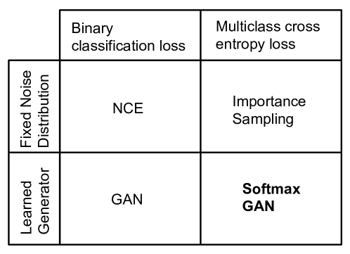
Note that Importance Sampling itself is strongly connected to NCE. As pointed out by [7] and [12], both Importance Sampling and NCE are training the underlying generative model with a classification surrogate. The difference is that in NCE, a binary classification task is defined between true and noise samples with a logistic loss, whereas Importance Sampling replaces the logistic loss with a multiclass softmax and cross-entropy loss. We show the relationship between NCE, Importance Sampling, GAN and this work in Figure 1. Softmax GAN is filling the table with the missing item.
4.4 Infinite batch size
As pointed out by [3], biased Importance Sampling estimation converges to the real partition function when the number of samples in one batch goes to infinity. In practice, we found that setting is enough for generating images that are visually realistic.
5 Experiments
We run experiments on image generation with the celebA database. We show that although Softmax GAN is minimizing the Jensen Shannon divergence between the generated data and the real data, it is more stable than the original GAN, and is less prone to mode collapsing.
We implement Softmax GAN by modifying the loss function of the DCGAN code (https://github.com/carpedm20/DCGAN-tensorflow). As DCGAN is quite stable, we remove the empirical techniques applied in DCGAN and observe instability in the training. On the contrary, Softmax GAN is stable to these changes.
5.1 Stablized training
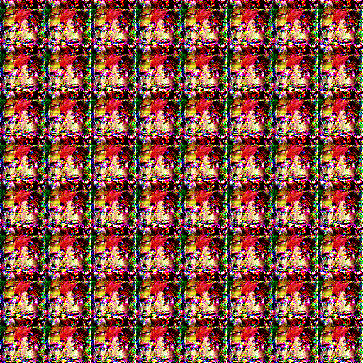
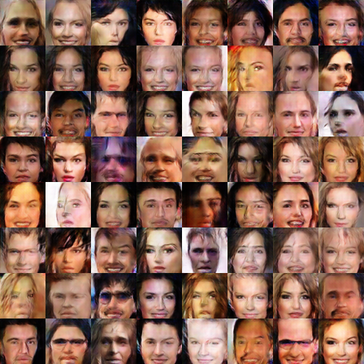
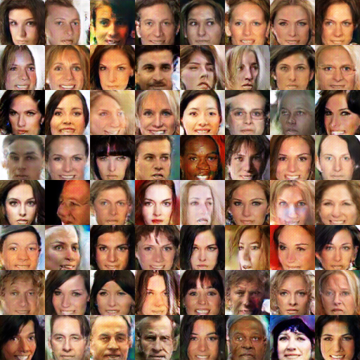
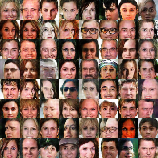
We follow the WGAN paper, by removing the batch normalization layers and using a constant number of filters in the generator network. We compare the results from GAN and Softmax GAN. The results are shown in Figure 2.
5.2 Mode collapse
When GAN training is not stable, the generator may generate samples similar to each other. This lack of diversity is called mode collapse because the generator can be seen as sampling only from some of the modes of the data distribution.
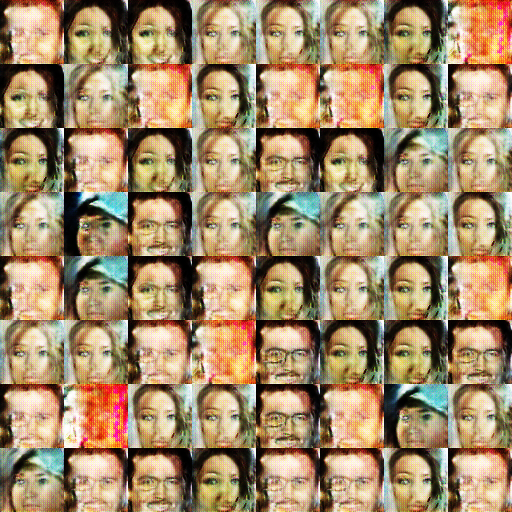
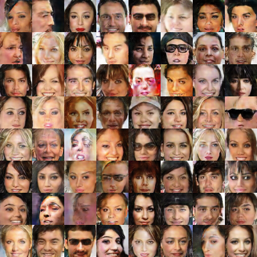
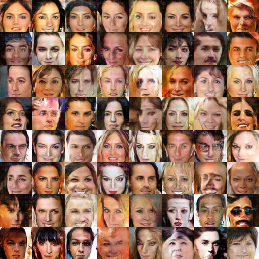
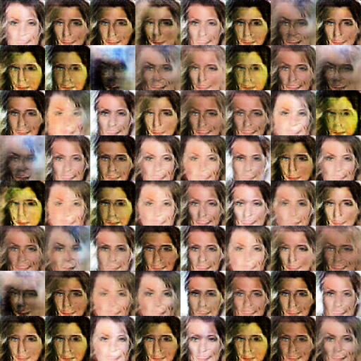
In the DCGAN paper, the pixels of the input images are normalized to . We remove this constraint and instead normalize the pixels to . At the same time, we replace the leaky relu with relu, which makes the gradients more sparse (this is unfavorable for GAN training according to the DCGAN authors). Under this setting, the original GAN suffers from a significant degree of mode collape and low image qualities. In contrast, Softmax GAN is robust to this change. Examplars are show in Figure 3.
5.3 Balance of generator and discriminator
It is claimed in [11] that manually balancing the number of iterations of the discriminator and generator is a bad idea. The WGAN paper however gives the discriminator phase more iterations to get a better discriminator for the training of the generator. We set the discriminator vs generator ratio to and and explore the effects of the this ratio on DCGAN and Softmax GAN. The results are in Figure 4 and 5 respectively.
6 Conclusions and future work
We propose a variant of GAN which does softmax across samples in a minibatch, and uses cross-entropy loss for both discriminator and generator. The target is to assign all probability to real data for discriminator and to assign probability equally to all samples for the generator. We proved that this objective approximately optimizes the JS-divergence using Importance Sampling. We futhur form the links between GAN, NCE, Importance Sampling and Softmax GAN. We demonstrate with experiments that Softmax GAN consistently gets good results when GAN fails at the removal of empirical techniques.
In our future work, we’ll perform a more systematic comparison between Softmax GAN and other GAN variants and verify whether it works on tasks other than image generation.
References
- [1] Martin Arjovsky, Soumith Chintala, and Léon Bottou. Wasserstein gan. arXiv preprint arXiv:1701.07875, 2017.
- [2] Yoshua Bengio et al. Quick training of probabilistic neural nets by importance sampling. In AISTATS, 2003.
- [3] Yoshua Bengio and Jean-Sébastien Senécal. Adaptive importance sampling to accelerate training of a neural probabilistic language model. IEEE Transactions on Neural Networks, 19(4):713–722, 2008.
- [4] Ian Goodfellow, Jean Pouget-Abadie, Mehdi Mirza, Bing Xu, David Warde-Farley, Sherjil Ozair, Aaron Courville, and Yoshua Bengio. Generative adversarial nets. In Z. Ghahramani, M. Welling, C. Cortes, N. D. Lawrence, and K. Q. Weinberger, editors, Advances in Neural Information Processing Systems 27, pages 2672–2680. Curran Associates, Inc., 2014.
- [5] Ian J Goodfellow. On distinguishability criteria for estimating generative models. arXiv preprint arXiv:1412.6515, 2014.
- [6] Michael Gutmann and Aapo Hyvärinen. Noise-contrastive estimation: A new estimation principle for unnormalized statistical models. In AISTATS, volume 1, page 6, 2010.
- [7] Rafal Jozefowicz, Oriol Vinyals, Mike Schuster, Noam Shazeer, and Yonghui Wu. Exploring the limits of language modeling. arXiv preprint arXiv:1602.02410, 2016.
- [8] Xudong Mao, Qing Li, Haoran Xie, Raymond YK Lau, and Zhen Wang. Least squares generative adversarial networks. arXiv preprint ArXiv:1611.04076, 2016.
- [9] Sebastian Nowozin, Botond Cseke, and Ryota Tomioka. f-gan: Training generative neural samplers using variational divergence minimization. In Advances in Neural Information Processing Systems, pages 271–279, 2016.
- [10] Guo-Jun Qi. Loss-sensitive generative adversarial networks on lipschitz densities. arXiv preprint arXiv:1701.06264, 2017.
- [11] Alec Radford, Luke Metz, and Soumith Chintala. Unsupervised representation learning with deep convolutional generative adversarial networks. arXiv preprint arXiv:1511.06434, 2015.
- [12] Sebastian Ruder. On word embeddings - part 2: Approximating the softmax. http://sebastianruder.com/word-embeddings-softmax/index.html#similaritybetweennceandis. Accessed: 2017-04-08.
- [13] Tim Salimans, Ian Goodfellow, Wojciech Zaremba, Vicki Cheung, Alec Radford, and Xi Chen. Improved techniques for training gans. In Advances in Neural Information Processing Systems, pages 2226–2234, 2016.