Explosive synchronization transition in a ring of coupled oscillators

Abstract

Explosive synchronization(ES), as one kind of abrupt dynamical transition in nonlinearly coupled systems, is currently a subject of great interests. Given a special frequency distribution, a mixed ES is observed in a ring of coupled phase oscillators which transit from partial synchronization to ES with the increment of coupling strength. The coupling weight is found to control the size of the hysteresis region where asynchronous and synchronized states coexist. Theoretical analysis reveals that the transition varies from the mixed ES, to the ES and then to a continuous one with increasing coupling weight. Our results are helpful to extend the understanding of the ES in homogenous networks.

Explosive synchronization transitions in large number of coupled complex network have been a hot topic since it is related to many inner regimes of collective dynamics and emergency phenomena. Although explosive synchronization in heterogeneous networks are commonly observed, the formation of it in homogeneous networks is still far beyond understanding. A kind of mixed explosive synchronization is firstly observed in the ring of coupled phase oscillators with a special frequency distribution where the coupled oscillators transit from partial synchronization to explosive synchronization with the increasing coupling strength. We further report on the effects of coupling weight on controlling the extent of the hysteretic region of coexistence of the unsynchronized and synchronized states. Theoretical analysis are presented to reveal the transition processes from mixed explosive synchronization, explosive synchronization and then to the continues transition with the effects of coupling weight. Our results are helpful to understand the regimes of explosive synchronization in homogenous networks.

I Introduction

Synchronization, as one of the commonly observed collective behavior in coupled oscillators, is a hot subject in nonlinear science since it is related to self-organization in both science and engineering applications such as neurons, fireflies, or cardiac pacemakers 1 . Inspired by the research on the small-world or scale-free networks, various synchronization dynamics in complex networks have been widely studied wang . Generally, two types of transition from incoherent to coherent state may exist in oscillators coupled with complex network structure: abrupt percolation and continuous phase transition. The former one, named as ES, was observed in scale-free networks of phase oscillators 2 ; 3 and chaotic oscillators4 . Kim et al. 5 explored the ES in the human brain networks and have tried to explain how it emerges from unconsciousness in sleep and anesthesia. Skardal et al. 6 found that ES can be realized by introducing disordered frequency distribution in synthetic networks. To better disclose the general mechanism of ES in coupled oscillators, growing attentions have been paid on the network topology and generic dynamics of nodes. Recent works 7 ; 3 showed that positive (negative) correlation between the degrees and the natural frequencies of nodes may lead to ES (hierarchical synchronization) among oscillators in scale-free networks, which was experimentally verified in electronic circuits 8 ; 9 . ES can also be obtained for any given frequency distribution if the complex networks are constructed with the frequency disassortative of node degrees10 ; 11 . Thu et al. 12 revealed that only when both the degrees and frequencies of the nodes in a network are disassortative can the ES occur. Leyva et al. 9 revealed that the continuous transition may change to a sharp, discontinuous phase transition in complex network. Zheng et al. 13 found that frustration may enhance or delay the explosive transition . Up to now, the investigations on the mechanism and the ES was mainly focused on network structure14 ; 15 ; 16 , dynamics of nodes17 ; 18 ; 19 , effects of time-delay 20 ; 21 ; 22 ; 23 , and the coupling form11 ; 24 ; 25 . In a heterogeneous scale-free network, the ES is well understood, due to the positive correlation between degrees and oscillation frequencies.

Although ES in heterogeneous network are commonly observed, the necessary and sufficient condition for its formation is still unknown. Hou et al.26 verified that no ES can be observed by introducing positive correlation between node degrees and natural frequencies in ER networks. Leyva et al. 4 observed the ES dynamics in homogeneous Erdős-Rényi (ER) networks and all-to-all networks by using frequency dependent coupling weights. They presented the first precise conditions of ES in homogeneous networks. However, it is still unclear whether ES can be observed in a regular ring of coupled oscillators which is another common and simple network. Rich dynamics exist in a ring of coupled oscillators such as various kinds of pattern formations 27 and amplitude death 28 . In our previous work 29 , we observed abrupt partial synchronization in a ring of coupled oscillators when the nodes are specially arranged according to their frequencies. Meng Zhan et al. 30 extended the work of frequency configuration in a ring of coupled oscillators. Motivated by these results, it seems natural to generate ES with appropriate arrangement of nodes based on frequency configuration and to reveal the generic properties of ES in a ring of coupled phase oscillators.

The remainder of this paper is organized as follows. In Sec. II, we introduce the model of coupled phase oscillators and give the main results. In Sec. III, theoretical results are presented to reveal the parameter regime for the existence of mixed ES in coupled phase oscillators. In Sec. IV, the effects of coupling weights on the synchronization is numerically and theoretically studied. In Sec. V, we summarize our studies and point out possible further development along the line of current study.

II Model and results

Without lack of generality, we consider the most classical and simple Kuramoto model 31

$$\dot{\theta_{i}}(t)=\omega_{i}+\frac{\epsilon}{k_{i}+1}\sum_{j=1}^{N}A_{i,j}\sin(\theta_{j}-\theta_{i}),i=1,2...,N,$$ (1)

where $\theta_{i}$ is the phase of the $i$th oscillator ($i=1,2...,N$), $\omega_{i}$ is its associated natural frequency drawn from a frequency distribution $g(\omega)$($g(\omega)$ follows uniform distribution in $[0,1]$ for simplicity), $\epsilon$ is the coupling strength, $A_{i,j}$ is the adjacency matrix with $A_{i,j}=1$ if node i and node j has connection, otherwise $A_{i,j}=0$. $k_{i}$ is the degree of the $i$th oscillator. Here we only focus on the nearest-neighbor-coupled ring of oscillators (with $A_{i,(i+1)}=1,A_{(i-1),i}=1,i=2,...,N-1$, and $A_{N,1}=1,A_{1,N}=1$, otherwise $A_{i,j}=0$).

To measure the transition from incoherence to phase synchronization, a classical order parameter for the system provided by Eq. 1 is $r(t)=\frac{1}{N}|\sum_{i=1}^{N}e^{j\theta_{i}(t)}|$, and the level of synchronization can be measured according to the value of $R=<r(t)>_{T}$, with$<...>_{T}$ denoting time average over a large time span $T$ and $j=\sqrt{-1}$. When $R\approx 1$, the system reaches the completely synchronous state. Otherwise, when $R\approx 0$, the oscillator ensemble exhibits incoherence, and oscillators behave almost independently. With the increment of the coupling strength $\epsilon$, the coupled system undergoes a phase transition (second-order or first-order) from non-synchronous ($R\sim\frac{1}{\sqrt{N}}$) to synchronous state ($R\approx 1$). In the following, we will explore the conditions and the parameter regimes for the occurrence of the ES in a ring of coupled phase oscillators.

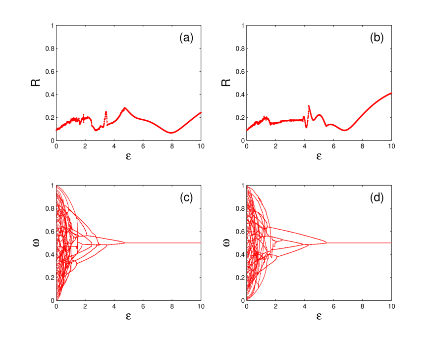
Figure 1: (color online) (a)(b) The average frequencies of all nodes versus coupling strength $\epsilon$ for $N=100$ with two arbitrary sets of frequencies.(c)(d) The numerical order parameter $R$ versus coupling strength $\epsilon$ corresponding to (a)(b),respectively.

For arbitrarily given frequency configuration of coupled phase oscillators, No ES dynamics are observed in a ring of coupled phase oscillators. The average frequencies of the coupled oscillators versus coupling strength $\epsilon$ are presented in Figs. 1(a) $\sim$ (b) for two arbitrary sets of random initial natural frequency configuration. Obviously, the synchronous transition process of the coupled oscillators is a continuous one since the final synchronous cluster is built up by combining several small synchronous clusters. Moreover, the corresponding order parameters $R$ also exhibit continues transitions as plotted in Figs. 1(c) $\sim$ (d). What should be mentioned is that the value of $R$ keeps small even when the oscillators are synchronized. The reason is that most of the oscillators are phase locked in anti-phase states in the ring of coupled oscillators. However, based on our former work 29 , we expect to observe ES in a ring of coupled phase oscillator when the necessary coupling strength for synchronization is small with the special frequency arrangement. For simplicity, we first set the frequency of node $i$ to be $\omega_{i}=\frac{i-1}{N-1},i=1,2,...,N$, then rearrange them to a special configuration with large roughness $Ro=\frac{1}{N}\sum^{N}_{=1}(\omega_{i+1}-\omega_{i})^{2}$ 29 as shown in Fig. 2(a) which is more precisely given by the following equation.

$$\left\{\begin{array}[]{lll}\omega_{i}&=&\frac{N-1+(-1)^{i}(2i-1)}{2(N-1)},i\leq\frac{N}{2},\\ \omega_{i}&=&1-\omega_{N+1-i},i>\frac{N}{2}\end{array},i=1,2...,N.\right.$$ (4)

In the above configuration, the oscillators are split into two groups where one group has relatively large mismatches between pair of neighboring nodes while the other one has relatively small mismatches. We will see how an explosive transition is generated in a system of size $N$ with the given frequency distribution. The order parameter exhibits two stages of transition when the coupling strength varies from 0 to 1. In the first stage, the order parameter is linearly increasing with the increment of coupling strength. In the second stage, the order parameter sharply transits to around 1 with an associated hysteresis part as shown in Fig. 2(b). By checking the average frequencies of all nodes versus coupling strength as shown in Fig. 2(c), we find that a sequence of nodes with smaller frequency mismatches $\delta\omega_{i}=\omega_{i}-\bar{\omega}$ firstly combines into one synchronization cluster whose average frequency $\bar{\omega}$ is 0.5. Then all the rest get annexed into the synchronous cluster in a sudden when the coupling strength is larger than the transition point. Since the synchronous transition is following a partial synchronization, we name the whole transition processes as the mixed ES. The occurrence of the mixed ES is not limited to the special initial natural frequency. When the initial frequencies of nodes before rearrangement are randomly selected, the mixed ES still can be observed if the final frequency distribution is rearranged with the characteristic of having maximal value of the roughness Ro and being strictly symmetric with respect to the average frequency of the whole coupled system. Fig. 2(d)-(f) present one example of random selection of the frequencies where the mixed ES can be observed according to the order parameter R and the average frequency versus coupling strength.

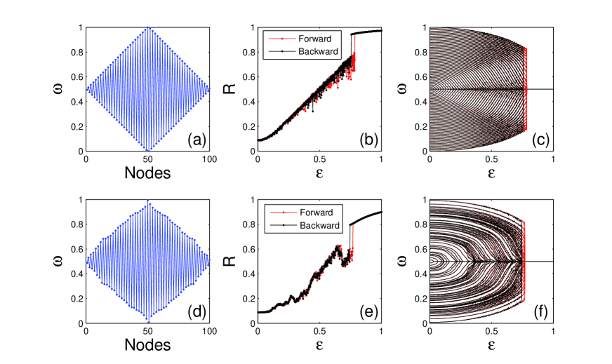
Figure 2: (color online) (a) The optimal configuration of the natural frequency based on Eq. 4 of $N=100$ coupled phase oscillators. (b) The order parameter $R$ versus the coupling strength $\epsilon$. The results are recorded by quasi-stationary method where the red lines depict the forward results (increasing $\epsilon$) while the black lines depict the backward results(decreasing $\epsilon$). (c) The average speeds of all nodes versus the coupling strength $\epsilon$ corresponding to (b). The second row shows the result of the random selection of the frequencies. (d)The rearranged frequency distribution with maximal roughness $Ro$ for one example of randomly set initial frequencies. (e) The order parameter $R$ versus the coupling strength $\epsilon$ for the new set of frequency distribution. (f) The average frequencies of all nodes versus the coupling strength $\epsilon$ corresponding to (e).

III Theoretical analysis

To better understand the dynamics of the ring of coupled oscillators with the special frequency distribution, we write Eq. 1 as

$$\dot{\theta_{i}}(t)=\omega_{i}+\frac{1}{3}\epsilon\Omega_{i},$$ (5)

where

$$\Omega_{i}=\sin(\theta_{i+1}-\theta_{i})+\sin(\theta_{i-1}-\theta_{i}).$$ (6)

According to Eq. 4, $|\omega_{i-1}-\omega_{i+1}|=\frac{2}{N-1}$. $\omega_{i-1}\approx\omega_{i+1}$ for large $N$. Then $\sin(\theta_{i+1}-\theta_{i})\approx\sin(\theta_{i-1}-\theta_{i})$ when nodes $i$,$i-1$,$i+1$ are in a synchronous cluster. Therefore,

$$\Omega_{i}\approx 2\sin(\theta_{i+1}-\theta_{i}).$$ (7)

When all nodes are in synchronous cluster, according to the natural character of the sine function ($|\sin x|\leq 1$), the boundary values of $\Omega_{i}$ (here defined as $\Omega_{bws}$ for convenience) satisfies

$$\Omega_{bws}=2.$$ (8)

Based on Eq. 5, if node $i$ is in the synchronous cluster, then the average frequency of the synchronous cluster can be defined as $\bar{\omega}=<\dot{\theta_{i}}>_{T}$ (here $\bar{\omega}=0.5$ for given frequency distribution in Eq. 4 ). Eq. 5 becomes

$$\Omega_{i}=\frac{3}{\epsilon}(\bar{\omega}-\omega_{i}).$$ (9)

Then the natural frequency of node $i$ in the synchronous cluster with average frequency $\bar{\omega}$ satisfies Eq. 10 for given coupling strength.

$$|\frac{3}{\epsilon}(\bar{\omega}-\omega_{i})|\leq\Omega_{bws}.$$ (10)

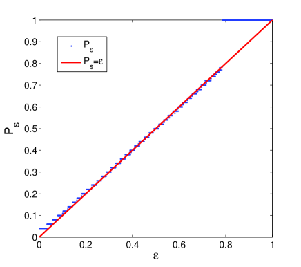
Figure 3: (color online) The portion of synchronous nodes versus coupling strength $\epsilon$ for $N=100$. The red lines depict the linear function $y=a*x$ with the parameter $a=1.000\pm 0.0016$ within $95\%$ confidence intervals.

It should be mentioned that the Eq. 10 is fulfilled only when all nodes are in synchronous clusters. Otherwise, the nodes on the boundary of synchronous cluster would be pulled out of the cluster by the neighboring non-synchronous nodes. Therefore, when the coupled oscillators are in partially synchronous state, the boundary value of $\Omega_{i}$ must be smaller than $\Omega_{bws}$ due to the influence of outer non-synchronous nodes. In order to figure out the actual boundary value of $\Omega_{i}$ for partially synchronous state, we numerically explore the transition process from incoherent to partial synchronization and try to explore the influence of the non-synchronous nodes on the synchronous nodes. The results indicate that the proportion of the synchronized nodes $P_{s}=\frac{N_{s}}{N}$ is equal to $\epsilon$, as shown in Fig. 3, for all $\epsilon$ before the ES. Moreover, the $N_{s}$ nodes in the synchronous cluster are those whose natural frequencies are near the value of $\bar{\omega}(=0.5)$. Define the maximal initial nature frequency of nodes in the synchronous cluster to be $\omega_{Smax}$, then the maximal deviation between natural frequency of nodes and the actual frequency of synchronous cluster can be described as $\delta\omega_{s}=\omega_{Smax}-\bar{\omega}$. Therefore, according to Eq. 4, the frequencies of all $N_{s}$ partially synchronous nodes are in the range as shown in Eq. 11.

$$|\omega_{i}-\bar{\omega}|\leq\frac{\delta\omega_{s}}{2}=\frac{\epsilon}{2},$$ (11)

When the coupled system is in partial synchronization, the actual boundary values of $\Omega_{i}$ is

$$|\Omega_{i}|=\frac{3}{\epsilon}|\bar{\omega}-\omega_{i}|\leq\frac{3}{\epsilon}\times\frac{\epsilon}{2}=1.5$$ (12)

For convenience, we defined $\Omega_{bps}=1.5$ to be the boundary of $\Omega_{i}$ for partial synchronous clusters, then the actual boundary of $\sin(\theta_{i+1}-\theta_{i})$ satisfies

$$|\sin(\theta_{i+1}-\theta_{i})|\leq\frac{\Omega_{bps}}{2}=0.75.$$ (13)

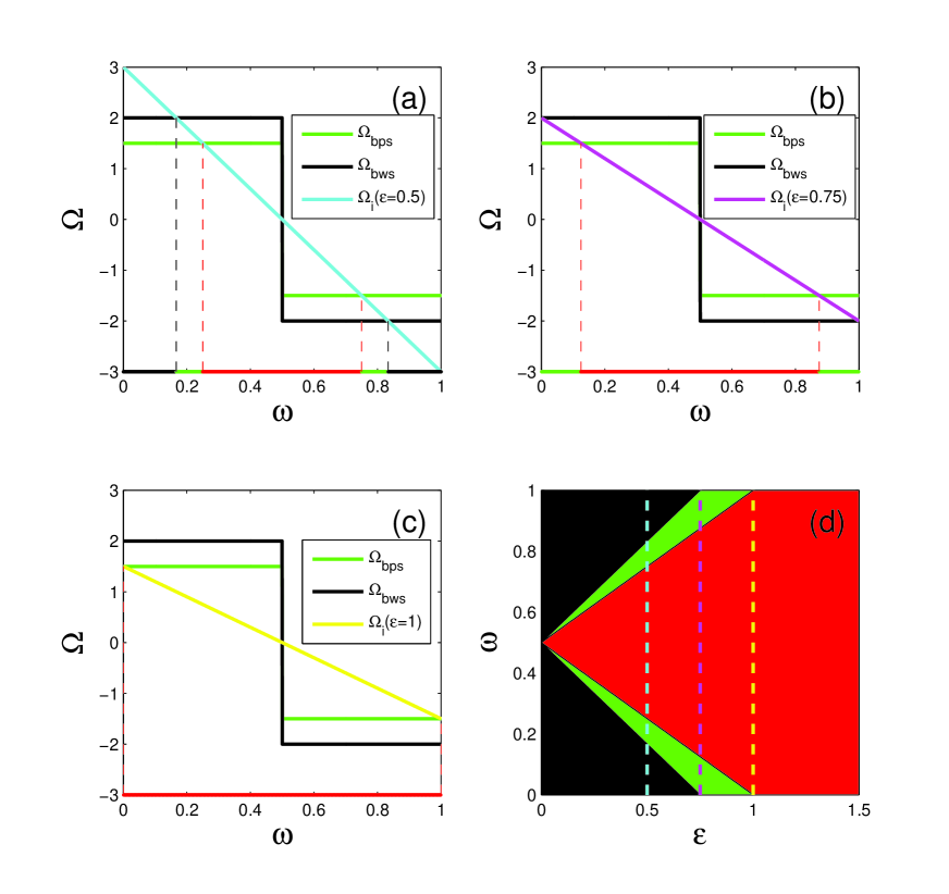
Figure 4: (color online) (a)(b)(c) The boundary lines of the full $\Omega_{bws}$ (black lines) and the partial synchronization $\Omega_{bps}$ (green lines), and $\Omega_{i}$ versus natural frequency $\omega_{i}$ for $\epsilon=0.5$(cyan lines), $\epsilon=0.75$(pink lines),$\epsilon=1.0$(yellow lines). (d) Three types of states as: non-synchronous (black), buffer (green), and synchronous state(red) in the parameter space of $\omega$ versus $\epsilon$.

Based on the two boundary values of $\Omega_{bps}$ and $\Omega_{bws}$, the nodes in the coupled system can be classified into three types, (1) partially synchronized nodes whose frequencies $\omega_{i}$ satisfy $|\Omega_{i}|<\Omega_{bps}$; (2) non-synchronous nodes whose frequencies $\omega_{i}$ satisfy $|\Omega_{i}|>\Omega_{bws}$; (3) buffer nodes whose frequencies $\omega_{i}$ satisfy $\Omega_{bps}<|\Omega_{i}|<\Omega_{bws}$. It is worth mentioning that the fate of the buffer nodes is determined by the competition between synchronous and non-synchronous group. If there are non-synchronous nodes in the coupled oscillator system, the buffer nodes keep away from the synchronous cluster, otherwise, if the outer non-synchronous nodes disappear, then the buffer nodes can join the synchronous cluster or stay unsynchronized, which depends on the initial conditions of those buffer nodes.

To better exhibit the fate of all coupled nodes, we plot the boundaries of the full synchronization $\Omega_{bws}$(black lines), partial synchronization $\Omega_{bps}$ (green lines), and the curve of $\Omega_{i}$ (blue lines) versus $\omega_{i}$ in Figs. 4(a) $\sim$ (c) for given $\epsilon=0.5,0.75,1.0$, respectively. Obviously, for given $\epsilon$, the slope of the curve $\Omega_{i}$ is determined ($|\Omega_{i}|=\frac{3}{\epsilon}|\bar{\omega}-\omega_{i}|$). Therefore, the fate of the nodes is clearly determined by the boundary lines and the slope of the curve $\Omega_{i}$. If the frequency $\omega_{i}$ of nodes $i$ satisfies $|\Omega_{i}|<\Omega_{bps}$, then the nodes whose frequencies are within the range between the two intersection points of the boundary lines of $\Omega_{bps}$ and $\Omega_{i}$ are partially synchronized (the frequencies of those nodes are marked with red dots). If $|\Omega_{i}|>\Omega_{bws}$, then nodes are in the non-synchronous state as marked with black dots. If $\Omega_{bps}<|\Omega_{i}|<\Omega_{bws}$, then the nodes may go either to the synchronous or the non-synchronous state depending on the motion of its neighboring nodes and its initial values (marked with green dots). The synchronization transition are plotted in the parameter space of $\omega\sim\epsilon$ as shown in Fig. 4(d) where the red, green, and black areas marks the synchronous, the buffer, and the non-synchronous nodes, respectively. What should be mentioned is that the fate of nodes in the green area will finally become the non-synchronous state if its neighboring nodes are in the non-synchronous states (black area for $\epsilon<0.75$). However, when there are no non-synchronous nodes for $\epsilon>0.75$, the fate of the buffer nodes can be either in the synchronous state if the initial condition is near the synchronous manifold or in the non-synchronous state if the initial condition is far away from the manifold otherwise, which builds up the bistable hysteresis area.

According to the analysis above, with the increment of the coupling strength, the transition from the incoherent to the synchronized state can be well described by the order parameter $R$. Since the phase of incoherent oscillators are randomly distributed in $[0,2\pi]$, they have less contribution to the order parameter $R$. However, if the oscillators are in the partially synchronous state, their phase are locked within a range which contribute significantly to the order parameter $R$. Therefore the order parameter is approximately calculated as $R\approx R_{s}$, where $R_{s}$ is the contribution of the synchronous nodes. Suppose that there are $N_{s}$ nodes whose natural frequencies are $\omega_{i},i=1,2,...,N_{s}$ in the synchronous cluster with average frequency $\bar{\omega}$, then their phases satisfy Eq. 14. Moreover, the phase of the $N_{s}$ synchronous nodes would be locked to each other (i.e. $\theta_{i-1}\approx\theta_{i}$, and $\sin(\theta_{(i-1)}-\theta_{i})\approx\theta_{i-1}-\theta_{i}$ for $i=2,3,...,N_{s}$).

$$\bar{\omega}=\omega_{i}+\frac{\epsilon}{3}(\sin(\theta_{i-1}-\theta_{i})+\sin(\theta_{i+1}-\theta_{i})).$$ (14)

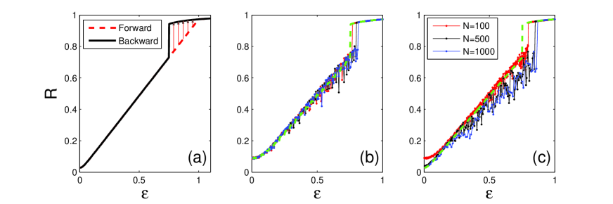
Figure 5: (color online) (a)The theoretical results of the order parameters R versus $\epsilon$. The red (black) lines are results for the forward (backward) one for N = 1000. (b)The numerical value of the order parameters of three arbitrary sets of initial conditions (red,black and blue) and the theoretical backward results (green dashed line) for N = 100. (c) The numerical value of the order parameters for system size N = 100(red dots),N = 500(black cross),N = 1000(blue circle) and the theoretical backward results (green dashed line) for N = 1000.

we get

$$\theta_{i-1}-2\theta_{i}+\theta_{i+1}=2\arcsin(\frac{3(\bar{\omega}-\omega_{i})}{2\epsilon}).$$ (15)

which determine the value of $\theta_{i},i=2,...,N_{s}$ for arbitrarily given $\theta_{1}$.

$$R\approx R_{s}=<\frac{1}{N}|\sum_{i=1}^{N_{s}}e^{j\theta_{i}}|>_{T}.$$ (16)

The order parameter $R$ can be determined according to Eq. 16 for the given number $N_{s}$ of nodes in the synchronous cluster. It is worth mentioning that $N_{s}$ are different upon increasing or decreasing the coupling strength based on the state distribution in Fig. 4 (d). When decreasing the coupling strength from $\epsilon=1.0$ to zero, $N_{s}$ is equal to the number of the nodes in the red and green area for $\epsilon>0.75$, since the nodes in green area (buffer nodes) start near the synchronous manifold and thus get finally synchronized. However, $N_{s}$ becomes the number of nodes in the red area when $\epsilon<0.75$ where the buffer nodes are always in the non-synchronous state. However, if the coupling strength increases from $\epsilon=0$ to 1, $N_{s}$ remains equal to the number of nodes in the red area and the buffer nodes stay away from the synchronous manifolds when non-synchronous nodes are nearby the buffer nodes. However, when the non-synchronous nodes nearby the buffer nodes disappear, the buffer nodes may join into the synchronous cluster without the influence of non-synchronous nodes. However, when it will jump to synchronous cluster is completely depending on the initial value of the coupled nodes which make it difficult to predict the jump point. Therefore, $N_{s}$ can be the number of nodes in the red area ($N_{r}$) in Fig. 4(d) or become N all at a sudden for any coupling strength $\epsilon$ between $[0.75,1.0)$. We can only predict the boundary value of R before the buffer nodes jumped to synchronous in a sudden by setting $N_{s}=N_{r}$ as shown the dashed lines in Fig. 5(a). The numerical evidences shown that the jump point are related to the initial value of the coupled phase oscillators as shown in Fig. 5(b) for $N=100$ coupled oscillators. Moreover, the jump point is also related to the system size according to plot of the order parameter versus $\epsilon$ for $N=100,500,1000$ as shown in Fig. 5(c). Therefore, the buffer nodes may join the synchronous cluster in a sudden when the remaining buffer nodes are less than a certain number $m$ which results in an earlier jump of the order parameter $R$. Moreover, the value of $m$ is related to the system size and the initial value of the coupled oscillators.

IV Influence of coupling weight on ES dynamics

It has been shown that the generalized Kuramoto model with frequency-weighted coupling can generate first-order synchronization transition in general networks 4 ; 25 . The effects of coupling weight on the transition process in a ring of coupled oscillators are non-trivial. It is convinient to control the transition process by introducing proper coupling weight. To reveal the influence of the weights on the transition process, coupling weights are introduced into the Kuramoto model similar as that in the complex network4 .

$$\dot{\theta_{i}}(t)=\omega_{i}+\frac{\epsilon}{k_{i}+1}\sum_{j=1}^{N}A_{i,j}|{\omega_{j}-\omega_{i}}|^{\alpha}\sin(\theta_{j}-\theta_{i}),i=1,2...,N,$$ (17)

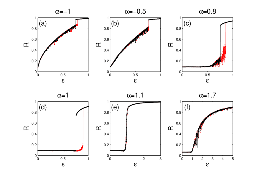
Figure 6: (color online) (a)-(f) The numerical results of the order parameter for the forward (red) and backward (black) traversal at different coupling weight $\alpha=-1.0,-0.5,0.8,1.0,1.1,1.7$, respectively.

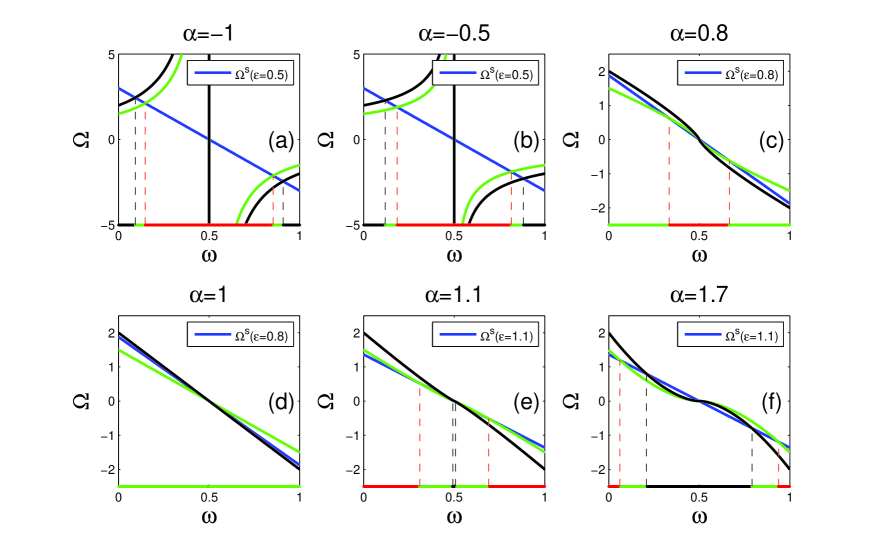
Figure 7: (color online) (a)-(f) The boundary lines of the whole synchronization $\Omega_{bws}$ (black lines) and partial synchronization $\Omega_{bps}$ (green lines), and the curves of $\Omega_{i}$ (blue lines) versus natural frequency $\omega_{i}$ for different coupling weight coefficients $\alpha=-1.0,-0.5,0.8,1.0,1.1,1.7$.

where $A_{i,j}$ is the same as that in Eq. 1. By increasing the value of $\alpha$ from 0 to 1 or decreasing it from 0 to -1, the transition process looks quite different. In the latter case, the mixed ES still exists while the boundary curve of the transition region changes from linear to convex, leading to the shrinkage of the area of the bistable part. However, in the former case, the boundary curve becomes concave, resulting in an expansion of the area. When $\alpha=1$, the mixed ES turns into a pure ES. However, it becomes continuous for $\alpha$ slightly larger than $1$. The dependence on $\alpha$ of the transition process is displayed in Figs. 6(a)-(f) for $\alpha=-1,-0.5,0.8,1.0,1.1,1.7$.

The coupling weight exponent $\alpha$ will change the number of nodes $N_{s}$ in the synchronous cluster as shown in Fig. 6. The $|\Omega_{i}|$ at the full synchronization for arbitrarily given $\alpha$ can be written as

$$\Omega_{bws}=(|\omega_{i+1}-\omega_{i}|^{\alpha}+|\omega_{i-1}-\omega_{i}|^{\alpha}),$$ (18)

while the transition curve to the partial synchronization is determined by

$$\Omega_{bps}=0.75(|\omega_{i+1}-\omega_{i}|^{\alpha}+|\omega_{i-1}-\omega_{i}|^{\alpha}).$$ (19)

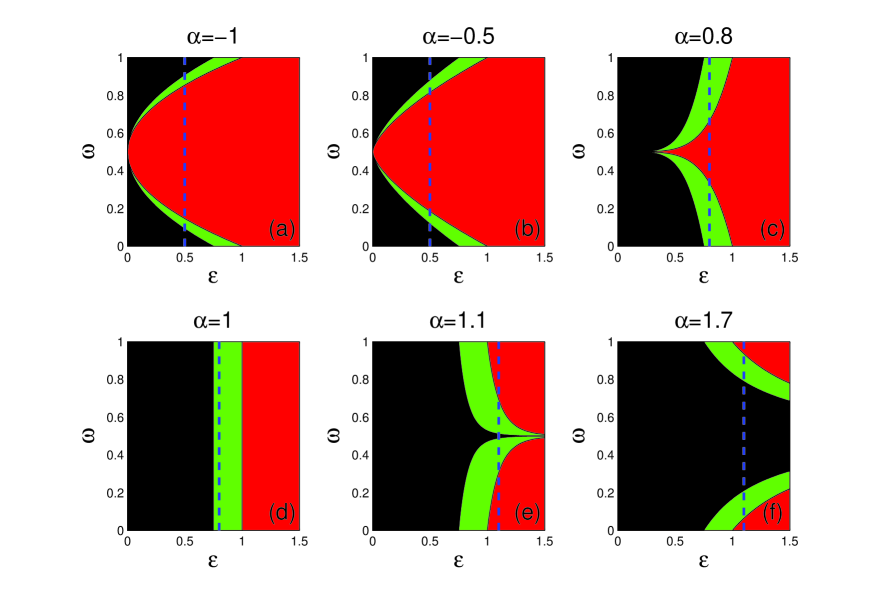
Figure 8: (color online) (a)-(f) Three types of states as: the non-synchronous (black), the buffer (green), and the synchronous state(red) in the parameter space of $\omega$ versus $\epsilon$ for different coupling weight exponents $\alpha=-1.0,-0.5,0.8,1.0,1.1,1.7$.

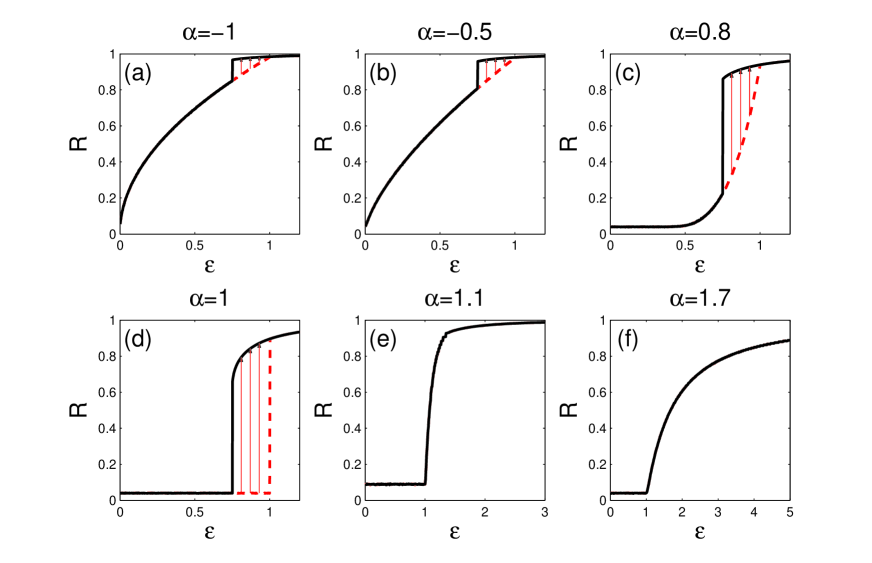
Figure 9: (color online) (a)-(f) The order parameters $R$ in the forward (red) and backward (black) direction versus $\epsilon$ for different coupling weight exponents $\alpha=-1.0,-0.5,0.8,1.0,1.1,1.7$.

Therefore, the coupling weight exponent $\alpha$ changes the shapes of boundary line $\Omega_{bws}$ and $\Omega_{bps}$ as shown in Figs. 7(a)-(f) for $\alpha=-1,-0.5,0.8,1.0,1.1,1.7$. Two horizontal lines of $\Omega_{bws}$ and $\Omega_{bps}$ at $\alpha=0$ become hyperbolic for negative $\alpha$, convex for $\alpha\in(0,1)$, and concave for $\alpha>1.0$. According to Eq. 9, the coupling strength $\epsilon$ determines the slope of $\Omega_{i}$ for each $\omega_{i}$. The synchronous nodes (red dots),buffer nodes(green dots), and the non-synchronous nodes (black dots) are classified by the two boundary lines and the slope of the line $\Omega_{i}$ as shown in Figs. 7(a)-(f). Those with frequency near $\bar{\omega}$ will get to the synchronous cluster quickly if $\alpha<1$. On the contrary, those with frequency away from $\bar{\omega}$ will get to the synchronous cluster first if $\alpha>1$. Nevertheless, if $\alpha=1$, all nodes get to synchronization simultaneously which leads to ES.

The dependence on $\alpha$ of the synchronous process in the parameter space of $\omega\sim\epsilon$ for $\alpha=-1,-0.5,0.8,1.0,1.1,1.7$ is shown in Figs. 8(a)-(f). The red, green, and black area denotes the synchronous, the buffer, and the non-synchronous state. The red area increases (decreases) by changing its shape from triangle to bell (cone) when $\alpha$ varies from $0$ to some negative (positive) values. When $\alpha=1$, the system makes a transition from the non-synchronous to the bistable and finally to the synchronous state as the coupling strength $\epsilon$ increases from $0$ to $1$, which finally leads to the ES. When $\alpha$ is slightly larger than $1$ (for example $\alpha=1.1$), the square area associated with the synchronous state is invaded by the cone-shaped buffer and the non-synchronous state. The number $N_{s}$ of the synchronized nodes can be extracted from Figs. 8(a)-(f) for given $\alpha$ and $\epsilon$. Based on Eqs. 15,16, the order parameter $R$ for $\alpha=-1.0,-0.5,0.8,1.0,1.1,1.7$ are calculated with the same method as those in Fig. 5(a) and shown in Figs. 9(a)-(f). The theoretical results again match well with the numerics.

V Discussion and conclusion

In conclusion, we have firstly observed a kind of mixed ES dynamics in the ring of a coupled phase oscillators by introducing a special frequency configuration of nodes. With this configuration, the coupled oscillators transit from partial synchronization to ES with the increment of the coupling strength. Generally, the coupling strength required for the synchronization of two coupled oscillators increases with the increment of their frequency mismatch. Therefore, those nodes whose frequencies are near the average get to synchronization first and form a synchronous cluster. The mixed ES dynamics can be well understood by the competition between three types of nodes (non-synchronous, buffer and synchronized nodes) in the nearest-neighbor coupled phase oscillators. In the partial synchronization process, the interaction between the non-synchronous and the synchronous nodes is transmitted by the buffer nodes, so that the increasing coupling strength tends to increase the number of the synchronous nodes while decreasing the non-synchronous ones. Once the non-synchronous nodes diminished, the competition exists only between the synchronous and the buffer nodes, so that the buffer nodes may stay non-synchronous or join into the synchronous cluster in a sudden depending on their initial condition and system size. As a result, the system transits dynamics change from partial synchronization to ES.

Upon introducing the coupling weight, the dynamics of the coupled phase oscillators are determined by the competition between the frequency mismatch and the coupling weight. With the negative coupling weight exponent $\alpha$, the larger frequency mismatch, the more weakly coupled the two nodes are. Since the negative coupling weight exponent $\alpha$ increases the effective coupling, the synchronous (non-synchronous) nodes increase (decrease) for a given coupling strength $\epsilon$, which leads to a larger order parameter. On the contrary, the positive coupling weight exponent $\alpha$ acts oppositely, which leads to a smaller order parameter. As the coupling weight exponent $\alpha=1$, the effective coupling strength is proportional to the frequency mismatch, which makes all nodes have the same critical coupling strength to get synchronization. Therefore, we observe the ES but not the partial synchronization. As $\alpha>1$, the nodes with larger frequency mismatch have larger coupling strength which again makes it easier to get synchronization than those with smaller frequency mismatch. The ES dynamics is thus not possible and replaced by a continuous transition.

Our results are based on the special frequency distribution. In order to realize ES or mixed ES, it is necessary to avoid multi-synchronous clusters. Therefore, the frequency distribution must be strictly symmetric with respect to the average frequency of the whole coupled system. Moreover, the nodes whose frequencies are near the average frequency must be spatially near each other. The frequencies of nodes can be randomly selected so long as they fulfill the two conditions above. Our results may help understand the synchronization in more complex networks with homogenous coupling and shed light on the control of pattern formation dynamics of coupled oscillators32 ; 33 ; 34 .

- (1) A. Pikovsky, M. Rosenblum, and J. Kurths, Synchronization A Universal Concept in Nonlinear Sciences (Cambridge University Press, Cambridge, England, 2001).
- (2) W. Lin, H. Fan, Y. Wang, H. Ying, and X. Wang, Controlling synchronous patterns in complex networks, Phys. Rev. E 93, 042209 (2016)
- (3) P. Ji, T. K. Peron, P. J. Menck, F. A. Rodrigues, and J. Kurths, Cluster Explosive Synchronization in Complex Networks, Phys. Rev. Lett. 110, 218701 (2013).
- (4) J. Gomez-Gardenes, S. Gomez, A. Arenas, and Y. Moreno, Explosive synchronization transitions in scalefree networks, Phys. Rev. Lett. 106, 128701 (2011).
- (5) I. Leyva, I. Sendina-Nadal, J. A. Almendral, A. Navas, S. Olmi, and S. Boccaletti, Explosive synchronization in weighted complex networks, Phys. Rev. E 88, 042808 (2013).
- (6) M. Kim, G. A. Mashour, S. B. Moraes, G. Vanini, V. Tarnal, E. Janke, A. G. Hudetz, and U. Lee, Functional and Topological Conditions for Explosive Synchronization Develop in Human Brain Networks with the Onset of Anesthetic-Induced Unconsciousness, Front. Comput. Neurosci. (2016).
- (7) P. S. Skardal and A. Arenas, Disorder induces explosive synchronization, Phys. Rev. E 89(6), 062811 (2014).
- (8) W. Liu, Y. Wu, J. Xiao, and M. Zhan, Effects of frequency-degree correlation on synchronization transition in scale-free networks, Europhys. Lett. 101,38002 (2013)
- (9) X. Hu, S. Boccaletti, W. Huang, X. Zhang, Z. Liu, S. Guan, and C. Lai, Exact solution for first-order synchronization transition in a generalized Kuramoto model, Sci. Rep. 4. 7262 (2014).
- (10) I. Leyva, R. Sevilla-Escoboza, J. M. Buldu, I. Sendina-Nadal, J. Gomez-Gardenes, A. Arenas, Y. Moreno, S. Gomez, R. Jaimes-Reategui, and S. Boccaletti, Explosive first-order transition to synchrony in networked chaotic oscillators, Phys. Rev. Lett. 108,168702 (2012).
- (11) P. Li, K. Zhang, X. Xu, J. Zhang, and M. Small, Reexamination of explosive synchronization in scale-free networks: The effect of disassortativity, Phys. Rev. E 87, 042803 (2013).
- (12) I. Leyva, A. Navas, I. Sendina-Nadal, J. A. Almendral, J. M. Buldu, M. Zanin, D. Papo, and S. Boccaletti, Explosive transitions to synchronization in networks of phase oscillators, Sci. Rep. 3, 1281 (2013).
- (13) L. Zhu, L. Tian, and D. Shi, Criterion for the emergence of explosive synchronization transitions in networks of phase oscillators, Phys. Rev. E 88, 042921 (2013)
- (14) C. Xu, J. Gao, H. Xiang, W. Jia, S. Guan, and Z. Zheng, Dynamics of phase oscillators with generalized frequency-weighted coupling, Phys. Rev. E 94, 062204 (2016).
- (15) X. Zhang, S. Boccaletti, S. Guan, and Z. Liu, Explosive synchronization in adaptive and multilayer networks, Phys. Rev. Lett. 114,038701 (2015).
- (16) P. Ji, T. K. Peron, F. A. Rodrigues, and J. Kurths, Analysis of cluster explosive synchronization in complex networks, Phys. Rev. E 90, 062810 (2014).
- (17) A. Navas, J. A. Villacorta-Atienza, I. Leyva, J. A. Almendral, I. Sendia-Nadal, and S. Boccaletti, Effective centrality and explosive synchronization in complex networks, Phys. Rev. E 92, 062820 (2015).
- (18) W. Zhou, L. Chen, H. Bi, X. Hu, Z. Liu, and S. Guan, Explosive synchronization with asymmetric frequency distribution, Phys. Rev. E 92, 012812 (2015).
- (19) R. S. Pinto and A. Saa, Explosive synchronization with partial degree-frequency correlation, Phys. Rev. E 91, 022818 (2015).
- (20) I. Sendia-Nadal, I. Leyva, A. Navas, J. A. Villacorta-Atienza, J. A. Almendral, Z. Wang, and S. Boccaletti, Effects of degree correlations on the explosive synchronization of scale-free networks, Phys. Rev. E 91, 032811 (2015).
- (21) T. K. Peron and F. A. Rodrigues, Explosive synchronization enhanced by time-delayed coupling, Phys. Rev. E 86, 016102(2012).
- (22) E. J. Friedman and A. S. Landsberg, Construction and analysis of random networks with explosive percolation, Phys. Rev. Lett. 103, 255701 (2009).
- (23) F. Radicchi and S. Fortunato, Explosive percolation in scale-free networks, Phys. Rev. Lett. 103, 168701 (2009).
- (24) Y. S. Cho, J. S. Kim, J. Park, B. Kahng, and D. Kim, Percolation transitions in scale-free networks under the Achlioptas process, Phys. Rev. Lett. 103, 135702 (2009).
- (25) C. Xu, J. Gao, Y. Sun, X. huang, and Z. Zheng, Explosive or Continuous: Incoherent state determines the route to synchronization, Sci. Rep. 5. 12039 (2015).
- (26) X. Zhang, X. Hu, J. Kurths, and Z. Liu, Explosive synchronization in a general complex network, Phys. Rev. E. 88, 010802(R) (2013).
- (27) H. Chen, G. He, F. Huang, C. Shen, and Z. Hou, Explosive synchronization transitions in complex neural networks, Chaos 23, 033124 (2013).
- (28) S. Liu, G. Zhang, Z. He, and M. Zhan, Optimal configuration for vibration frequencies in a ring of harmonic oscillators: The nonidentical mass effect, Front. Phys. 10, 100503 (2015)
- (29) J. Yang, Transitions to amplitude death in a regular array of nonlinear oscillators, Phys. Rev. E 76, 016204 (2007).
- (30) Y. Wu, J. Xiao, G. Hu, and M. Zhan, Synchronizing large number of nonidentical oscillators with small coupling, Europhys. Lett. 97,40005 (2012).
- (31) Y. Zhang, G. Hu, and H. A. Cerdeira, How does a periodic rotating wave emerge from high-dimensional chaos in a ring of coupled chaotic oscillators, Phys. Rev. E 64, 037203 (2001)
- (32) Y. Kuramoto, Chemical Oscillations, Waves, and Turbulencef (Springer, Berlin, 1984).
- (33) W. Lin, H. Fan, Y. Wang, H. Ying, and X. Wang, Controlling synchronous patterns in complex networks, Phys. Rev. E 93, 042209 (2016).
- (34) Z. Song, C. Y. Ko, M. Nivala, J. N. Weiss, and Z. Qu, Calcium-voltage coupling in the genesis of early and delayed afterdepolarizations in cardiac myocytes, Biophys. J. 108 1908(2015).
- (35) Z. Song, A. Karma, J. N. Weiss, and Z. Qu, Long-Lasting Sparks: Multi-Metastability and Release Competition in the Calcium Release Unit Network, PLoS Comput Biol 12: e1004671 (2016).