Human-in-the-Loop SLAM

Abstract

Building large-scale, globally consistent maps is a challenging problem, made more difficult in environments with limited access, sparse features, or when using data collected by novice users. For such scenarios, where state-of-the-art mapping algorithms produce globally inconsistent maps, we introduce a systematic approach to incorporating sparse human corrections, which we term Human-in-the-Loop Simultaneous Localization and Mapping (HitL-SLAM). Given an initial factor graph for pose graph SLAM, HitL-SLAM accepts approximate, potentially erroneous, and rank-deficient human input, infers the intended correction via expectation maximization (EM), back-propagates the extracted corrections over the pose graph, and finally jointly optimizes the factor graph including the human inputs as human correction factor terms, to yield globally consistent large-scale maps. We thus contribute an EM formulation for inferring potentially rank-deficient human corrections to mapping, and human correction factor extensions to the factor graphs for pose graph SLAM that result in a principled approach to joint optimization of the pose graph while simultaneously accounting for multiple forms of human correction. We present empirical results showing the effectiveness of HitL-SLAM at generating globally accurate and consistent maps even when given poor initial estimates of the map.

Introduction

Building large-scale globally consistent metric maps requires accurate relative location information between poses with large spatial separation. However, due to sensor noise and range limitations, such correlations across distant poses are difficult to extract from real robot sensors. Even when such observations are made, extracting such correlations autonomously is a computationally intensive problem. Furthermore, the order of exploration, and the speed of the robot during the exploration affect the numerical stability, and consequently the global consistency of large-scale maps. Due to these factors, even state of the art mapping algorithms often yield inaccurate or inconsistent large-scale maps, especially when processing data collected by novice users in challenging environments.

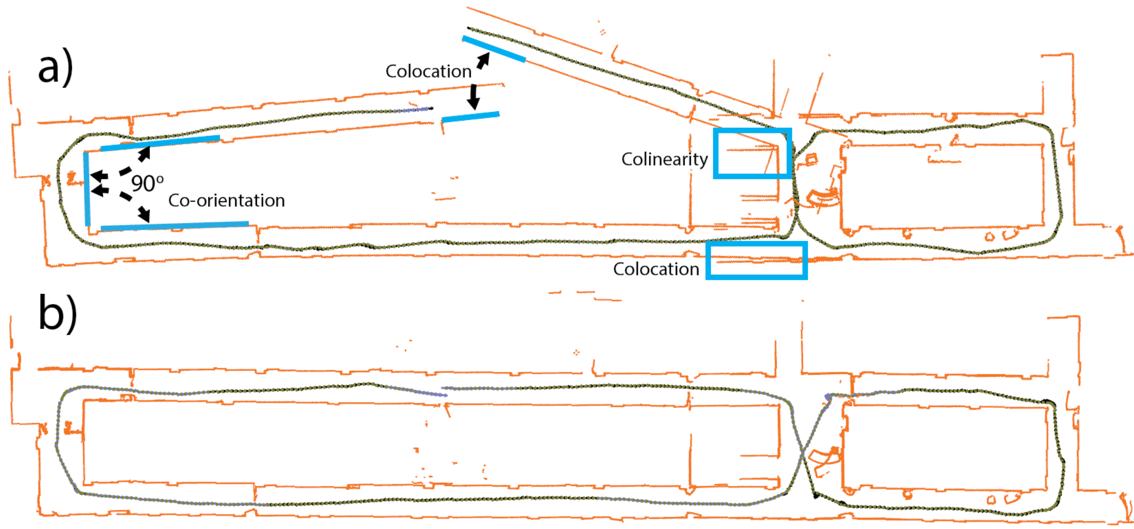
Figure 1: HitL SLAM example, showing a) the input initial map with global consistency errors, and b) the resulting final map produced by HitL-SLAM by incorporating human corrections (blue lines) along with the input.

To address these challenges and limitations of large-scale mapping, we propose Human-in-the-Loop SLAM (HitL-SLAM), a principled approach to incorporate approximate human corrections in the process of solving for metric maps. Fig. 1 presents an example of HitL-SLAM in practice. HitL-SLAM operates on a pose graph estimate of a map along with the corresponding observations from each pose, either from an existing state-of-the-art SLAM solver, or aligned only by odometry. In an interactive, iterative process, HitL-SLAM accepts human corrections, re-solves the pose graph problem, and presents the updated map estimate. This iterative procedure is repeated until the user is satisfied by the mapping result, and provides no further corrections.

We thus present three primary contributions: 1) an EM-based algorithm (?) to interpret several types of approximate human correction for mapping (§4), 2) a human factor formulation to incorporate a variety of types of human corrections in a factor graph for SLAM (§5), and 3) a two-stage solver for the resultant, hybrid factor graph composed of human and robot factors, which minimally distorts trajectories in the presence of rank deficient human corrections (§5). We show how HitL-SLAM introduces numerical stability in the mapping problem by using human corrections to introduce off-diagonal blocks in the information matrix. Finally, we present several examples of HitL-SLAM operating on maps that intrinsically included erroneous observations and poor initial map estimates, and producing accurate, globally consistent maps.

Related Work

Solutions to robotic mapping and SLAM have improved dramatically in recent years, but state-of-the-art algorithms still fall short at being able to repeatable and robustly produce globally consistent maps, particularly when deployed over large areas and by non-expert users. This is in part due to the difficulty of the data association problem  (?; ?; ?). The idea of humans and robots collaborating in the process of map building to overcome such limitations is not new, and is known as Human-Augmented Mapping (HAM).

Work within HAM belongs primarily to one of two groups, depending on whether the human and robot collaborate in-person during data collection (C-HAM), or whether the human provides input remotely or after the data collection (R-HAM). Many C-HAM techniques exist to address semantic  (?; ?) and topological  (?) mapping. A number of approaches have also been proposed for integrating semantic and topological information, along with human trackers  (?), interaction models  (?), and appearance information (?), into conceptual spatial maps  (?), which are organized in a hierarchical manner.

There are two limitations in these C-HAM approaches. First, a human must be present with the robot during data collection. This places physical constraints on the type of environments which can be mapped, as they must be accessible and traversable by a human. Second, these methods are inefficient with respect to the human’s attention, since most of the time the human’s presence is not critical to the robot’s function, for instance during navigation between waypoints. These approaches, which focus mostly on semantic and topological mapping, also typically assume that the robot is able to construct a nearly perfect metric map entirely autonomously. While this is reasonable for small environments, globally consistent metric mapping of large, dynamic spaces is still a hard problem.

In contrast, most of the effort in R-HAM has been concentrated on either incorporating human input remotely via tele-operation such as in the Urban Search and Rescue (USAR) problem  (?; ?), or in high level decision making such as goal assignment or coordination of multiple agents  (?; ?; ?). Some R-HAM techniques for metric mapping and pose estimation have also been explored, but these involve either having the robot retrace its steps to fill in parts missed by the human  (?) or by having additional agents and sensors in the environment  (?).

A number of other approaches have dealt with interpreting graphical or textual human input within the contexts of localization (?; ?) and semantic mapping (?). While these approaches solve similar signal interpretation problems, this paper specifically focuses on metric mapping.

Ideally, a robot could explore an area only once with no need for human guidance or input during deployment, and later with minimal effort, a human could make any corrections necessary to achieve a near-perfect metric map. This is precisely what HitL-SLAM does, and additionally HitL-SLAM does not require in-person interactions between the human and robot during the data collection.

Human-in-the-Loop SLAM

HitL-SLAM operates on a factor graph $G=\{X,F\}$, where $X$ is the set of estimated poses along the robot’s trajectory, and $F=\{R,H\}$ is the set of factors which encode information about both relative pose constraints arising from odometry and observations, $R$, and constraints supplied by the human, $H$. The initial factor graph $G_{0}$ may be provided by any pose graph SLAM algorithm, and HitL-SLAM is capable of handling constraints in $G_{0}$ with or without loop closure. In our experiments, we used Episodic non-Markov Localization (EnML) (?) without any explicit loop closures beyond the length of each episode.

HitL-SLAM runs iteratively, with the human specifying constraints on observations in the map, and the robot then enforcing those constraints along with all previous constraints to produce a revised estimate of the map. To account for inaccuracies in human-provided corrections, interpretation of the such input is necessary before human correction factors can be computed and added to the factor graph. Each iteration, the robot first proposes an initial graph $G_{i}=\{X_{i},F_{i}\}$, then the human supplies a set of correction factors $H_{i}$, and finally the robot re-optimizes the poses in the factor graph, producing $G_{i}^{\prime}=\{X_{i}^{\prime},F_{i}\cup H_{i}\}$.

Definition 1.

A human correction factor, h, is defined by the tuple $h=\langle P_{a},P_{b},S_{a},S_{b},X_{a},X_{b},m\rangle$ with:

$S_{a},S_{b}$ are subsets of all observations $S$, and poses $x_{i}$ are added to the sets $X_{a},X_{b}$ if there are observations in $S_{a},S_{b}$ that arising from pose $x_{i}$. $M$ is an enumeration of the modes of human correction, a subset of which are shown in Fig. 2. The modes $M$ of correction are defined as follows:

1. Colocation: A full rank constraint specifying that two sets of observations are at the same location, and with the same orientation.

2. Collinearity: A rank deficient constraint specifying that two sets of observations are on the same line, with an unspecified translation along the line.

3. Perpendicularity: A rank deficient constraint specifying that the two sets of observations are perpendicular, with an unspecified translation along either of their lines.

4. Parallelism: A rank deficient constraint specifying that the two sets of observations are parallel, with an unspecified translation along the parallel lines.

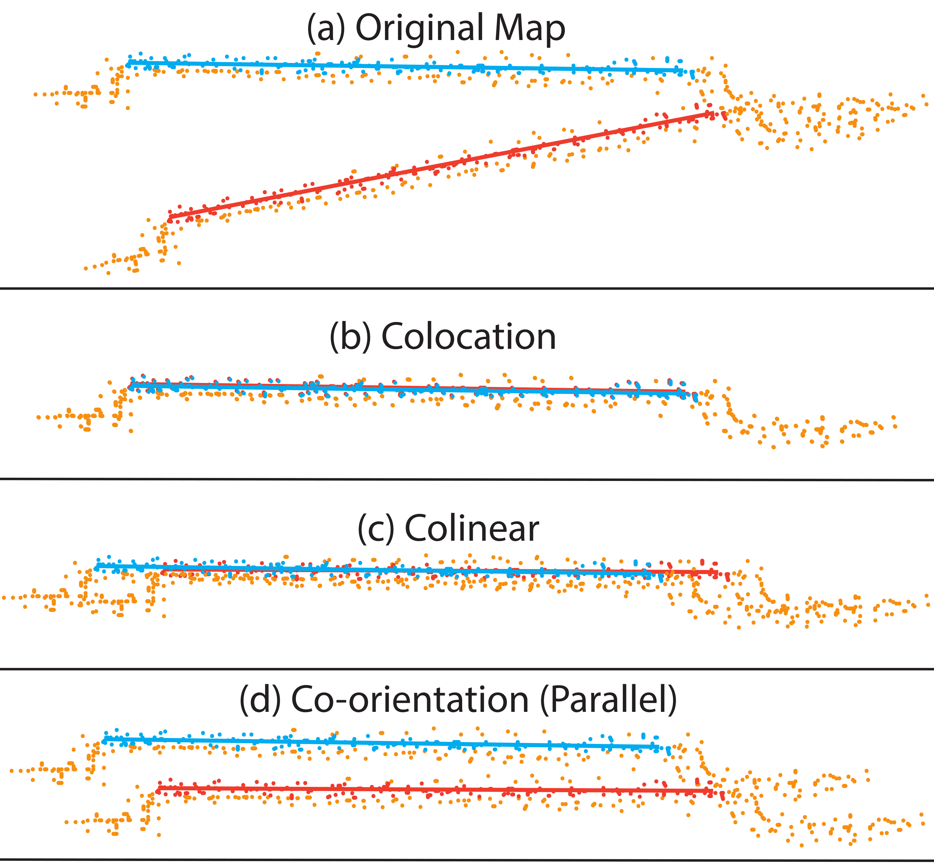
Figure 2: Result of transforming observation point clouds based on different human constraints, showing (a) Original map, (b) Colocation constraint, (c) Collinear constraint, (d) Co-orientation constraint. In all sub-figures the red and blue lines denote $P_{a}$ and $P_{b}$, respectively, and red and blue points denote $S_{a}$ and $S_{b}$. $S\setminus(S_{a}\cup S_{b})$ appear in orange.

Each iteration of HitL-SLAM proceeds in two steps, shown in Fig. 3. First, the human input is gathered, interpreted, and a set of human correction factors are instantiated (Block 1). Second, a combination of analytical and numerical techniques is used to jointly optimize the factor graph using both the human correction factors and the relative pose factors (Block 2). The resulting final map may be further revised and compressed by algorithms such as Long-Term Vector Mapping (?).

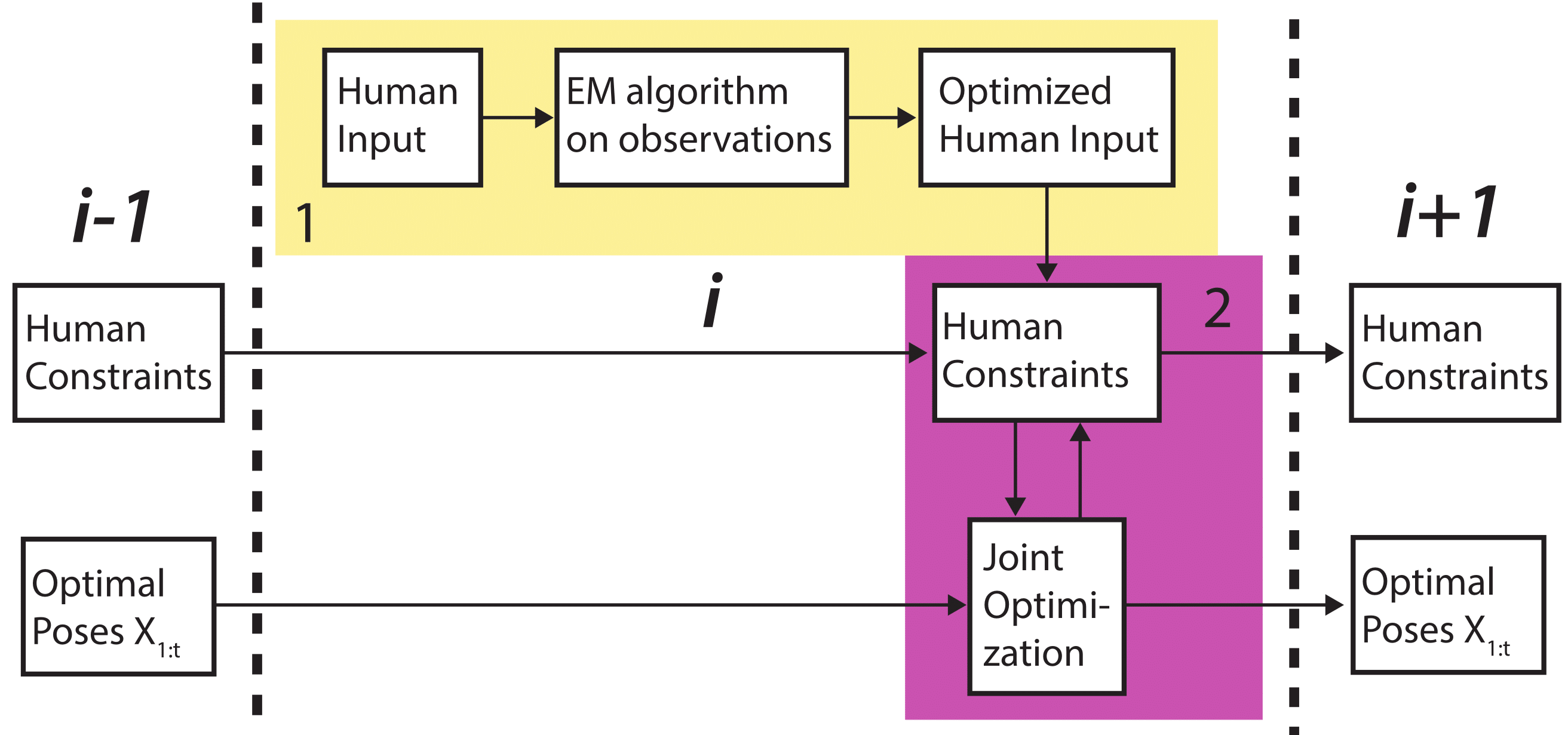
Figure 3: Flow of information during processing of the $i^{\text{th}}$ human input. Block 1 (yellow) outlines the evaluation of human input, and block 2 (purple) outlines the factor graph construction and optimization processes. Note that the joint optimization process optimizes both pose parameters and human constraint parameters.

We model the problem of interpreting human input as finding the observation subsets $S_{a},S_{b}$ and human input sets $P_{a},P_{b}$ which maximize the joint correction input likelihood, $p(S_{a},S_{b},P_{a},P_{b}|P_{a}^{0},P_{b}^{0},m)$, which is the likelihood of selecting observation sets $S_{a},S_{b}$ and point sets $P_{a},P_{b}$, given initial human input $P_{a}^{0},P_{b}^{0}$ and correction mode $m$. To find $S_{a},S_{b}$ and $P_{a},P_{b}$ we use the sets $P_{a}^{0},P_{b}^{0}$ and observations in a neighborhood around $P_{a}^{0},P_{b}^{0}$ as initial estimates in an Expectation Maximization approach. As the pose parameters are adjusted during optimization in later iterations of HitL-SLAM, the locations of points in $P_{a},P_{b}$ may change, but once an observation is established as a member of $S_{a}$ or $S_{b}$ its status is not changed.

Once $P_{a},P_{b}$ and $S_{a},S_{b}$ are determined for a new constraint, then given $m$ we can find the set of poses $X^{*}_{1:t}$ which best satisfy all given constraints. We first compute an initial estimate $X^{0}_{1:t}$ by analytic back-propagation of the most recent human correction factor, considering sequential constraints in the pose-graph. Next, we construct and solve a joint optimization problem over the relative pose factors $r$ and the human correction factors $h$. This amounts to finding the set of poses $X^{*}_{1:t}$ which minimize the sum of the cost of all factors,

$$X^{*}_{1:t}=\operatorname*{argmin}_{X_{1:t}}\left[\sum_{i=1}^{|R|}c_{r}(r_{i})+\sum_{j=1}^{|H|}c_{m}(h_{j})\right],$$

where $c_{r}:R\rightarrow\mathbb{R}$ computes the cost from relative pose-graph factor $r_{i}$, and $c_{m}:H\rightarrow\mathbb{R}$ computes the cost from human correction factor $h_{j}$ with correction mode $m$. Later sections cover the construction of the human correction factors and the formulation of the optimization problem.

Interpreting Human Input

Human Input Interface

HitL-SLAM users provide input by first entering the ‘provide correction’ state by pressing the ‘p’ key. Once in the ‘provide correction’ state, they enter points for $P_{a}$, $P_{b}$ by clicking and dragging along the feature (line segment) they wish to specify. The mode $m$ is determined by which key is held down during the click and drag. For instance, CTRL signifies a colocation constraint, while SHIFT signifies a collinear constraint. To finalize their entry, the user exits the ‘provide correction’ state by again pressing the ‘p’ key. Exit from the ‘provide correction’ state triggers the algorithm in full, and the user may specify additional corrections once a revised version of the map is presented.

Human Input Interpretation

Due to a number of factors including imprecise input devices, screen resolution, and human error, what the human actually enters and what they intend to enter may differ slightly. Given the raw human input line segment end-points $P_{a}^{0},P_{b}^{0}$ and the mode of correction $m$, we frame the interpretation of human input as the problem of identifying the observation sets $S_{a},S_{b}$ and the effective line segment end-points $P_{a},P_{b}$ most likely to be captured by the potentially noisy points $P_{a}^{0},P_{b}^{0}$. To do this we use the EM algorithm, which maximizes the log-likelihood $\ell$,

$$\ell(\theta)=\sum_{i}\sum_{z_{i}}p(z_{i}|s_{i},\theta^{\text{old}})\log(p(z_{i},s_{i}|\theta)),$$

where the parameters $\theta=\{P_{a},P_{b}\}$ are the interpreted human input (initially assumed to be $P_{a}^{0},P_{b}^{0}$), the $s_{i}\in S$ are the observations, and the latent variables $z_{i}$ are indicator variables denoting the inclusion or exclusion of $s_{i}$ from $S_{a}$ or $S_{b}$. The expressions for $p(z_{i}|s_{i},\theta^{\text{old}})$ and $p(z_{i},s_{i}|\theta)$ come from a generative model of human error based on the normal distribution, $\mathcal{N}(\mu(\theta),\sigma^{2})$. Here, $\sigma$ is the standard deviation of the human’s accuracy when manually specifying points, and is determined empirically; $\mu(\theta)$ is the center or surface of the feature.

Let $\delta(s_{i},\theta)$ be the squared Euclidean distance between a given observation $s_{i}$ and the feature (in this case a line segment) parameterized by $\theta$. Note that $p(z_{i}|s_{i},\theta)$ is convex due to our Gaussian model of human error. Thus, the EM formulation reduces to iterative least-squares over changing subsets of $S$ within the neighborhoods of $P_{a},P_{b}$. The raw human inputs $P_{a}^{0},P_{b}^{0}$ are taken as the initial guess to the solution $\theta$, and are successively refined of iterations of the EM algorithm to compute the final interpreted human input $P_{a},P_{b}$.

Once $P_{a},P_{b}$ have been determined, along with observations $S_{a},S_{b}$, we can find the poses responsible for those observations $X_{a},X_{b}$, thus fully defining the human correction factor $h$. To make this process more robust to human error when providing corrections, a given pose is only allowed in $X_{a}$ or $X_{b}$ if there exist a minimum of $T_{p}$ elements in $S_{a}$ or $S_{b}$ corresponding to that pose. The threshold $T_{p}$ is used for outlier rejection of provided human corrections. It is empirically determined by evaluating a human’s ability to accurately select points corresponding to map features, and is the minimum number of points a feature must have for it to be capable of being repeatedly and accurately selected by a human.

Solving HitL-SLAM

After interpreting human input, new pose estimates are computed in three steps. First, all explicit corrections indicated by the human are made by applying the appropriate transformation to $X_{b}$ and subsequent poses. Next, any resultant discontinuities are addressed using Closed-Form Online Pose-Chain SLAM (COP-SLAM) (?). And last, final pose parameters are calculated via non-linear least-squares optimization of a factor graph. The three-step approach is necessary in order to avoid local minima.

Applying Explicit Human Corrections

Although the user may select sets of observations in any order, we define all poses $x_{i}\in X_{a}$ to occur before all poses $x_{j}\in X_{b}$. That is, $P_{a}$ is the input which selects observations $S_{a}$ arising from poses $X_{a}$ such that $\forall x_{i}\in X_{a}$ and $x_{j}\in X_{b}$, $i<j$, where $X_{b}$ is defined analogously by observations $S_{b}$ specified by input $P_{b}$.

Given $P_{a}$ and $P_{b}$, we find the affine correction transformation $A$ which transforms the set of points defined by $P_{b}$ to the correct location relative to the set of points defined by $P_{a}$, as specified by mode $m$. If the correction mode is rank deficient, we force the motion of the observations as a whole to be zero along the null space dimensions. For co-orientation, this means that the translation correction components of $A$ are zero, and for collinearity the translation along the axis of collinearity is zero. Fig. 2 shows the effect of applying different types of constraints to a set of point clouds.

After finding $A$ we then consider the poses in $X_{b}$ to constitute points on a rigid body, and transform that body by $A$. The poses $x_{k}$ such that $\forall x_{j}\in X_{b}$, $k>j$, are treated similarly, such that the relative transformations between all poses occurring during or after $X_{b}$ remain unchanged.

Error Backpropagation

If $X_{a}\cup X_{b}$ does not form a contiguous sequence of poses, then this explicit change creates at least one discontinuity between the earliest pose in $X_{b}$, $x^{b}_{0}$ and its predecessor, $x_{c}$. We define affine transformation $C$ such that $x^{b}_{0}=A_{cb}Cx_{c}$, where $A_{cb}$ was the original relative transformation between $x_{c}$ and $x_{0}^{b}$. Given $C$, and the pose and covariance estimates for poses between $X_{a}$ and $X_{b}$, we use COP-SLAM over these intermediate poses to transform $x_{c}$ without inducing further discontinuities.

The idea behind COP-SLAM is a covariance-aware distribution of translation and rotation across many poses, such that the final pose in the pose-chain ends up at the correct location and orientation. The goal is to find a set of updates $U$ to the relative transformations between poses in the pose-chain such that $C=\prod_{i=1}^{n}U_{i}$.

COP-SLAM has two primary weaknesses as a solution to applying human corrections in HitL-SLAM. First, it requires translation uncertainty estimates to be isotropic, which is not true in general. Second, COP-SLAM deals poorly with nested loops, where it initially produces good pose estimates but during later adjustments may produce inconsistencies between observations. This is because COP-SLAM is not able to simultaneously satisfy both current and previous constraints. Due to these issues, we use COP-SLAM as an initial estimate to a non-linear least-squares optimization problem, which produces a more robust, globally consistent map.

HitL-SLAM Optimization

Without loop closure, a pose-chain of $N$ poses has $\mathcal{O}(N)$ factors. With most loop closure schemes, each loop can be closed by adding one additional factor per loop. In HitL-SLAM, the data provided by the human is richer than most front-end systems, and reflecting this in the factor graph could potentially lead to a prohibitively large number of factors. If $|X_{a}|=n$ and $|X_{b}|=m$, then a naïve algorithm that adds a factor between all pairs $(x^{a}_{i},x^{a}_{j})$, $(x^{a}_{i},x^{b}_{j})$, and $(x^{b}_{i},x^{b}_{j})$, where $x^{a}\in X_{a}$ and $x^{b}\in X_{b}$, would add $(m+n)^{2}$ factors for every loop. This is a poor approach for two reasons. One, the large number of factors can slow down the optimizer and potentially prevent it from reaching the global optimum. And two, this formulation implies that every factor is independent of every other factor, which is incorrect.

Thus, we propose a method for reasoning about human correction factors jointly, in a manner which creates a constant number of factors per loop while also preserving the structure and information of the input. Given a human correction factor $h=\langle P_{a},P_{b},S_{a},S_{b},X_{a},X_{b},m\rangle$, we define $c_{m}$ as the sum of three residuals, $R_{a}$, $R_{b}$, and $R_{p}$. The definitions of $R_{a}$ and $R_{b}$ are the same regardless of the correction mode $m$:

$$R_{a}=\left(\frac{\sum_{i=1}^{|S_{a}|}\delta(s_{i}^{a},P_{a})}{|S_{a}|}\right)^{\frac{1}{2}},\hskip 1.42262ptR_{b}=\left(\frac{\sum_{i=1}^{|S_{b}|}\delta(s_{i}^{b},P_{b})}{|S_{b}|}\right)^{\frac{1}{2}}.$$

As before, $\delta(s,P)$ denotes the squared Euclidean distance from observation $s$ to the closest point on the feature defined by the set of points $P$. All features used in this study are line segments, but depending on $m$, more complicated features with different definitions for $\delta(s,P)$ may be used. $R_{a}$ implicitly enforces the interdependence of different $x_{a}\in X_{a}$, since moving a pose away from its desired relative location to other poses in $X_{a}$ will incur cost due to misaligned observations. The effect on $X_{b}$ by $R_{b}$ is analogous.

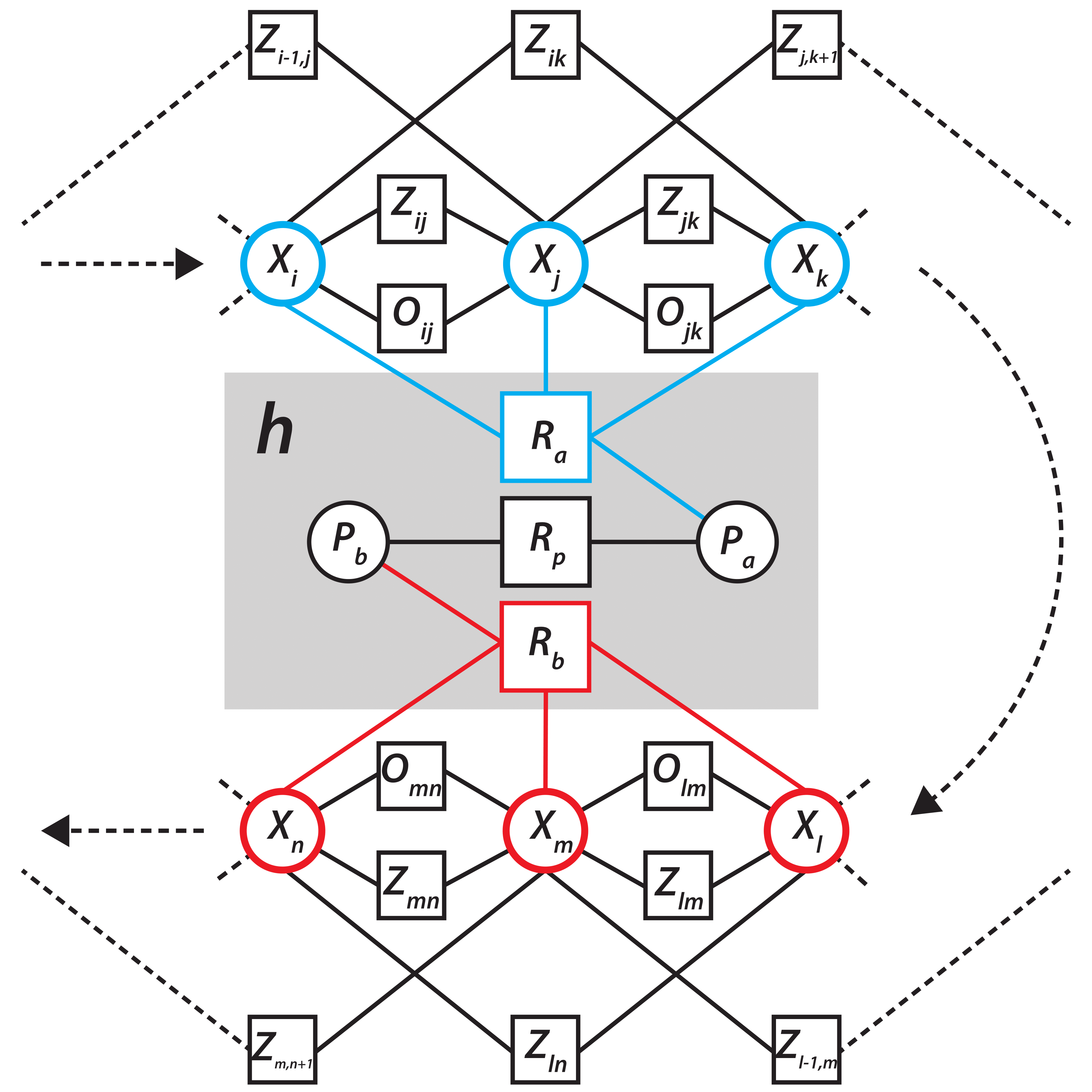
Figure 4: Subset of a factor graph containing a human factor $h$. Factors $R_{a}$ and $R_{b}$ drive observations in $S_{a}$ and $S_{b}$ toward features $P_{a}$ and $P_{b}$, respectively. Factor $R_{p}$ enforces the geometric relationship between $P_{a}$ and $P_{b}$. Note that parameters in $X_{a}$ (blue poses) and $X_{b}$ (red poses) as well as $P_{a}$ and $P_{b}$ are jointly optimized.

The relative constraints between poses in $X_{a}$ and poses in $X_{b}$ are enforced indirectly by the third residual, $R_{p}$. Depending on the mode, colocation ($+$), collinearity ($-$), co-orientation parallel ($\parallel$), co-orientation perpendicular ($\perp$), the definition changes:

$$R_{p}^{+} =K_{1}||cm_{b}-cm_{a}||+K_{2}(1-(\hat{n}_{a}\cdot\hat{n}_{b})),$$

$$R_{p}^{-} =K_{1}||(cm_{b}-cm_{a})\cdot\hat{n}_{a}||+K_{2}(1-(\hat{n}_{a}\cdot\hat{n}_{b})),$$

$$R_{p}^{\parallel} =K_{2}(1-(\hat{n}_{a}\cdot\hat{n}_{b})),$$

$$R_{p}^{\perp} =K_{2}(\hat{n}_{a}\cdot\hat{n}_{b}).$$

Here, $cm_{a}$ and $cm_{b}$ are the centers of mass of $P_{a}$ and $P_{b}$, respectively, and $\hat{n}_{a}$ and $\hat{n}_{b}$ are the unit normal vectors for the feature (line) defined by $P_{a}$ and $P_{b}$, respectively. $K_{1}$ and $K_{2}$ are constants that determine the relative costs of translational error ($K_{1}$) and rotational error ($K_{2}$). The various forms of $R_{p}$ all drive the points in $P_{b}$ to the correct location and orientation relative to $P_{a}$. During optimization the solver is allowed to vary pose locations and orientations, and by doing so the associated observation locations, as well as points in $P_{a}$ and $P_{b}$. Fig. 4 illustrates the topology of the human correction factors in our factor graph.

Note that HitL-SLAM allows human correction factors to be added to the factor graph in a larger set of situations compared to autonomous loop closure. HitL-SLAM introduces ‘information’ loop closure by adding correlations between distant poses without the poses being at the same location as in conventional loop closure. The off-diagonal elements in the information matrix thus introduced by HitL-SLAM assist in enforcing global consistency just as the off-diagonal elements introduced by loop closure. Fig. 5 further illustrates this point – note that the information matrix is still symmetric and sparse, but with the addition of off-diagonal elements from the human corrections.

Figure 5: Example map (a) with corrections and resulting information matrix (b). The white band diagonal represents the correlations from the initial factor graph $G_{0}$. The colored lines on the map show the human correction input: colocation (blue) and collinear (magenta).. The constraints correspond to the blue and magenta off-diagonal entries in the information matrix.

Figure 6: Initial and final maps from HitL-SLAM. Each map is of the same floor, and consists of between 600 and 700 poses. Maps in the left column (a) are initial maps, and maps in the right column (b) are final maps. Observations are shown in orange and poses are shown as arrows. Poses which are part of a human constraint are blue, while those which are not are in black.

Results

Figure 7: A large map a) corrected by HitL-SLAM b) using human correction, some of which are highlighted c). d) shows an approximate overlay of the map onto an aerial image of the complex from google earth. The map contains over 3000 poses.

Evaluation of HitL-SLAM is carried out through two sets of experiments. The first set is designed to test the accuracy of HitL-SLAM, and the second set is designed to test the scalability of HitL-SLAM to large environments.

To test the accuracy of HitL-SLAM, we construct a data set in a large room during which no two parallel walls are simultaneously visible to the robot. We do this by limiting the range of our robot’s laser to 1.5m so that it sees a wall only when very close. We then drive it around the room for which we have ground truth dimensions. This creates sequences of “lost” poses throughout the pose-chain which rely purely on odometry to localize, thus accruing error over time. We then impose human constraints on the resultant map and compare to ground truth, shown in Fig. 8. Note that the human corrections do not directly enforce any of the measured dimensions. The initial map shows a room width of 5.97m, and an angle between opposite walls of $4.1^{\circ}$. HitL-SLAM finds a room width of 6.31m, while the ground truth width is 6.33m, and produces opposite walls which are within $1^{\circ}$ of parallel. Note also that due to the limited sensor range, the global correctness must come from proper application of human constraints to the factor graph including the “lost” poses between wall observations.

To quantitatively evaluate accuracy on larger maps, where exact ground truth is sparse, we measured an inter-corridor spacing (Fig. 6 2b), which is constant along the length of the building. We also measured angles between walls we know to be parallel or perpendicular. The results for ground truth comparisons before and after HitL-SLAM, displayed in Table 1, show that HitL-SLAM is able to drastically reduce map errors even when given poor quality initial maps.

Figure 8: Initial a) and final b) maps for the ‘lost poses’ experiment. Observations are shown in orange, poses are black arrows, and ground truth (walls) is represented by the black lines. Poses involved in human constraints are colored blue.

We introduce an additional metric for quantitative map evaluation. We define the pair-wise inconsistency $I_{i,j}$ between poses $x_{i}$ and $x_{j}$ to be the area which observations from pose $x_{i}$ show as free space and observations from pose $x_{j}$ show as occupied space. We define the total inconsistency $\mathbf{I}$ over the map as the pair-wise sum of inconsistencies between all pairs of poses, $\mathbf{I}=\sum_{i=1}^{N-1}\sum_{j=i+1}^{N}I_{i,j}$. The inconsistency metric thus serves as a quantitative metric of global registration error between observations in the map, and allows us to track the effectiveness of global registration using HitL-SLAM over multiple iterations. The initial inconsistency values for maps LGRC 3A and 3B were $297.5m^{2}$ and $184.3m^{2}$, respectively. The final inconsistency values were $47.6m^{2}$ and $3.7m^{2}$, respectively, for an average inconsistency reduction of $91\%$ relative to the initial map, thus demonstrating the improved global consistency of the map generated using HitL-SLAM. Fig. 6 and Fig. 9 offer some qualitative examples of HitL-SLAM’s performance.

Map	Samples		Input Err.		HitL-SLAM Err.
	A	T	A(∘)	T(m)	A(∘)	T(m)
Lost Poses	10	4	3.1	0.07	1.0	0.02
LGRC 3A	14	10	9.8	3.3	1.5	0.06
LGRC 3B	14	10	7.6	3.1	1.1	0.02
BIG MAP	22	10	5.9	2.8	1.6	0.03
Mean	60	34	6.74	2.71	1.4	0.04

Table 1: Quantitative mapping errors using HitL-SLAM compared to ground truth, in the input maps, and after HitL-SLAM. The ‘Samples’ column denotes how many pairwise feature comparisons were made on the map and then compared to hand-measured ground truth. Angular (A) errors are in degrees, translation (T) errors in meters.

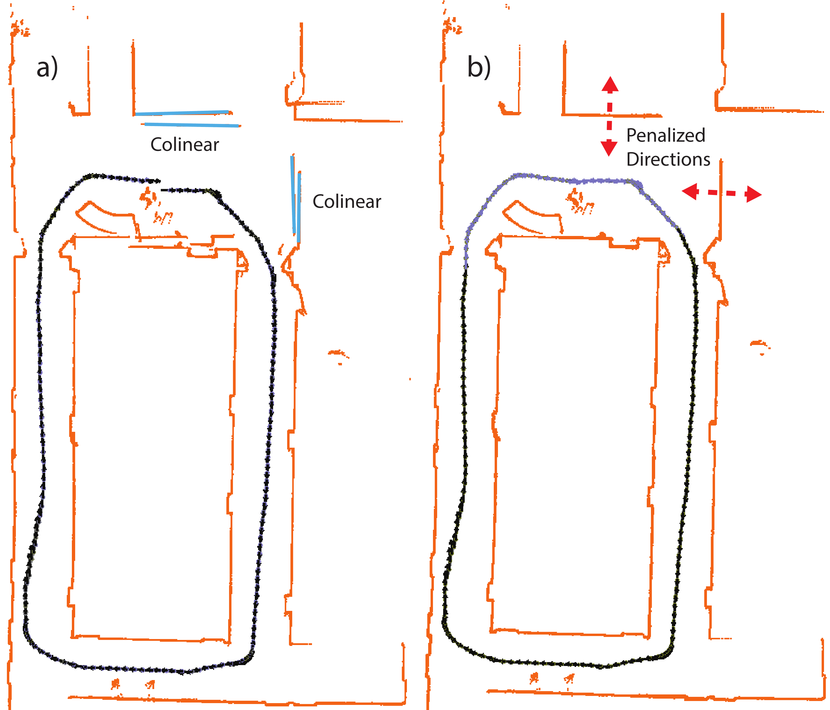
Figure 9: Example of how rank-deficient (collinear) constraints can be combined to effect a full rank constraint. Often, it is easier to tell if two sets of observations are collinear rather than colocated. Supporting rank-deficient constraints allows HitL-SLAM to operate on a larger set of maps.

To test the scalability of HitL-SLAM, we gathered several datasets with between 600 and 700 poses, and one with over 3000 poses and nearly 1km of indoor travel between three large buildings. Fig. 6 shows some of the moderately sized maps, and Fig. 7 details the largest map. 16 constraints were required to fix the largest map, and computation time never exceeded the time required to re-display the map, or for the human to move to a new map location.

All maps shown in Fig. 6 were corrected interactively by the human using HitL-SLAM in under 15 minutes. Furthermore, HitL-SLAM solves two common problems which are difficult or impossible to solve via re-deployment: 1) a severely bent hallway, in Fig. 6 1a), and 2) a sensor failure, in Fig. 6 2a) which caused the robot to incorrectly estimate its heading by roughly 30 degrees at one point. Combined, these results show that incorporating human input into metric mapping can be done in a principled, computationally tractable manner, which allows us to fix metric mapping consistency errors in less time and with higher accuracy than previously possible, given a small amount of human input.

Conclusion

We present Human-in-the-Loop SLAM (HitL-SLAM), an algorithm designed to leverage human ability and meta-knowledge as they relate to the data association problem for robotic mapping. HitL-SLAM contributes a generalized framework for interpreting human input using the EM algorithm, as well as a factor graph based algorithm for incorporating human input into pose-graph SLAM. Future work in this area could proceed towards further reducing the human requirements, and extending this method for higher dimensional SLAM and for different sensor types.

References

- [Aulinas et al. 2008] Aulinas, J.; Petillot, Y. R.; Salvi, J.; and Lladó, X. 2008. The slam problem: a survey. In CCIA, 363–371. Citeseer.
- [Bailey and Durrant-Whyte 2006] Bailey, T., and Durrant-Whyte, H. 2006. Simultaneous localization and mapping (slam): Part ii. IEEE Robotics & Automation Magazine 13(3):108–117.
- [Behzadian et al. 2015] Behzadian, B.; Agarwal, P.; Burgard, W.; and Tipaldi, G. D. 2015. Monte carlo localization in hand-drawn maps. In Intelligent Robots and Systems (IROS), 2015 IEEE/RSJ International Conference on, 4291–4296. IEEE.
- [Biswas and Veloso 2017] Biswas, J., and Veloso, M. M. 2017. Episodic non-markov localization. Robotics and Autonomous Systems 87:162–176.
- [Boniardi et al. 2016] Boniardi, F.; Valada, A.; Burgard, W.; and Tipaldi, G. D. 2016. Autonomous indoor robot navigation using a sketch interface for drawing maps and routes. In Robotics and Automation (ICRA), 2016 IEEE International Conference on, 2896–2901. IEEE.
- [Christensen and Topp 2010] Christensen, H. I., and Topp, E. A. 2010. Detecting region transitions for human-augmented mapping.
- [Dempster, Laird, and Rubin 1977] Dempster, A. P.; Laird, N. M.; and Rubin, D. B. 1977. Maximum likelihood from incomplete data via the em algorithm. Journal of the Royal Statistical Society. Series B (Methodological) 39(1):1–38.
- [Dissanayake et al. 2011] Dissanayake, G.; Huang, S.; Wang, Z.; and Ranasinghe, R. 2011. A review of recent developments in simultaneous localization and mapping. In 2011 6th International Conference on Industrial and Information Systems, 477–482. IEEE.
- [Doroodgar et al. 2010] Doroodgar, B.; Ficocelli, M.; Mobedi, B.; and Nejat, G. 2010. The search for survivors: Cooperative human-robot interaction in search and rescue environments using semi-autonomous robots. In Robotics and Automation (ICRA), 2010 IEEE International Conference on, 2858–2863. IEEE.
- [Dubbelman and Browning 2015] Dubbelman, G., and Browning, B. 2015. Cop-slam: Closed-form online pose-chain optimization for visual slam. IEEE Transactions on Robotics 31(5):1194–1213.
- [Hemachandra, Walter, and Teller 2014] Hemachandra, S.; Walter, M. R.; and Teller, S. 2014. Information theoretic question asking to improve spatial semantic representations. In 2014 AAAI Fall Symposium Series.
- [Kim et al. 2009] Kim, S.; Cheong, H.; Park, J.-H.; and Park, S.-K. 2009. Human augmented mapping for indoor environments using a stereo camera. In 2009 IEEE/RSJ International Conference on Intelligent Robots and Systems, 5609–5614. IEEE.
- [Kleiner, Dornhege, and Dali 2007] Kleiner, A.; Dornhege, C.; and Dali, S. 2007. Mapping disaster areas jointly: Rfid-coordinated slam by hurnans and robots. In 2007 IEEE International Workshop on Safety, Security and Rescue Robotics, 1–6. IEEE.
- [Milella et al. 2007] Milella, A.; Dimiccoli, C.; Cicirelli, G.; and Distante, A. 2007. Laser-based people-following for human-augmented mapping of indoor environments. In Artificial Intelligence and Applications, 169–175.
- [Murphy 2004] Murphy, R. R. 2004. Human-robot interaction in rescue robotics. IEEE Transactions on Systems, Man, and Cybernetics, Part C (Applications and Reviews) 34(2):138–153.
- [Nashed and Biswas 2016] Nashed, S., and Biswas, J. 2016. Curating long-term vector maps. In Intelligent Robots and Systems (IROS), 2016 IEEE/RSJ International Conference on, 4643–4648. IEEE.
- [Nieto-Granda et al. 2010] Nieto-Granda, C.; Rogers, J. G.; Trevor, A. J.; and Christensen, H. I. 2010. Semantic map partitioning in indoor environments using regional analysis. In Intelligent Robots and Systems (IROS), 2010 IEEE/RSJ International Conference on, 1451–1456. IEEE.
- [Nourbakhsh et al. 2005] Nourbakhsh, I. R.; Sycara, K.; Koes, M.; Yong, M.; Lewis, M.; and Burion, S. 2005. Human-robot teaming for search and rescue. IEEE Pervasive Computing 4(1):72–79.
- [Olson et al. 2013] Olson, E.; Strom, J.; Goeddel, R.; Morton, R.; Ranganathan, P.; and Richardson, A. 2013. Exploration and mapping with autonomous robot teams. Communications of the ACM 56(3):62–70.
- [Parasuraman et al. 2007] Parasuraman, R.; Barnes, M.; Cosenzo, K.; and Mulgund, S. 2007. Adaptive automation for human-robot teaming in future command and control systems. Technical report, DTIC Document.
- [Pronobis and Jensfelt 2012] Pronobis, A., and Jensfelt, P. 2012. Large-scale semantic mapping and reasoning with heterogeneous modalities. In Robotics and Automation (ICRA), 2012 IEEE International Conference on, 3515–3522. IEEE.
- [Topp and Christensen 2006] Topp, E. A., and Christensen, H. I. 2006. Topological modelling for human augmented mapping. In 2006 IEEE/RSJ International Conference on Intelligent Robots and Systems, 2257–2263. IEEE.
- [Topp et al. 2006] Topp, E. A.; Huettenrauch, H.; Christensen, H. I.; and Eklundh, K. S. 2006. Bringing together human and robotic environment representations-a pilot study. In 2006 IEEE/RSJ International Conference on Intelligent Robots and Systems, 4946–4952. IEEE.
- [Zender et al. 2007] Zender, H.; Jensfelt, P.; Mozos, O. M.; Kruijff, G.-J. M.; and Burgard, W. 2007. An integrated robotic system for spatial understanding and situated interaction in indoor environments. In AAAI, volume 7, 1584–1589.