Regular string-like braneworlds

Abstract

In this work, we propose a new class of smooth thick string-like braneworld in six dimensions. The brane exhibits a varying brane-tension and an $AdS$ asymptotic behavior. The brane-core geometry is parametrized by the Bulk cosmological constant, the brane width and by a geometrical deformation parameter. The source satisfies the dominant energy condition for the undeformed solution and has an exotic asymptotic regime for the deformed solution. This scenario provides a normalized massless Kaluza-Klein mode for the scalar, gravitational and gauge sectors. The near-brane geometry allows massive resonant modes at the brane for the $s$ state and nearby the brane for $l=1$.

I Introduction

The braneworld paradigm brought new geometrical solutions for some of the most intriguing problems in physics, as the hierarchy problem (rs1, ; rs2, ) and the origin of the dark energy (cosmology, ) and the dark matter (darkmatter, ). The warped geometry allows the bulk fields to propagate into an infinite extra dimension kehagias and provides rich internal structure for the brane (Bazeia, ). In five dimensions, the brane can be realized as a four dimensional domain wall, whose topological features guarantees the brane stability dewolfe ; gremm ; resonance .

In the codimension-2, the vortex scenarios are a suitable source for an axisymmetric brane, known as a string-like braneworld Olasagasti ; Gregory1 . By adding one more extra dimension to the Bulk spacetime, the correction to the Newtonian gravitational potential turns out to be smaller than in 5D Gherghetta . Moreover, in the thin string-like brane limit, no fine-tunning between the Bulk cosmological constant and the brane tension is needed Gherghetta . The conical behaviour nearby the brane also provides a mechanism for the brane cosmological problem (Kehagias:2004fb, ).

However, a global vortex geometry exhibits a mild singularity Cohen and a regular local Abelian 3-brane which satisfies the dominant energy condition Giovannini and a baby skyrmion brane Brihaye:2010nf which was only accomplished numerically. In the thin string-like brane limit, a vacuum $AdS_{6}$ traps the massless modes of the bosonic and fermionic fields and provides a smaller correction to the gravitational potential Gherghetta ; Tinyakov ; Oda1 ; Liufermions . By considering a vanishing Bulk cosmological constant, a braneworld with a supersymmetric scalar fields and a cigar shape was found cigaruniverse . Some brane-core geometries were proposed considering more involved transverse spaces, such as the soliton cigar stringcigar , the resolved conifold resolvedconifold , the catenoid (Torrealba, ), an apple shapped manifold appleshapped , the torus T2 and other.

In this article, we present a new class of smooth thick string-like model and explore some of its physical and geometrical features. The brane-tension varies inside the brane-core and attains the $AdS$ regime asymptotically. The inclusion of a deformation parameter enables a continuous flow from the thin string into a thick brane with a core structure. The deformation parameter modifies the core properties, such as the behaviour of the stress-energy components and the variation of the curvature inside the core. Among the thick string-like solutions, we analyzed the properties of two models: the first solution has a bell-shaped source satisfying the dominant energy and the second, whose source exhibits an exotic asymptotic behaviour. For the dynamics of bulk bosonic fields in these thick brane scenarios, the Kaluza-Klein modes reveal interesting near and far brane characteristics.

This work is organized as follows. In Sec. II we present the smooth and deformed solutions and study their source and geometry properties. In Sec. III, the Kaluza-Klein modes for the scalar, vector gauge and gravitational fields are studied and their features discussed. In Sec. IV, final remarks and perspectives are outlined.

II Smooth string-like geometries

Consider a six-dimensional spacetime $M_{6}$ whose bulk dynamic is governed by the Einstein Hilbert action with bulk cosmological constant $\Lambda$, namely Olasagasti ; Gregory1 ; Cohen ; Oda1 ; Oda2 ; Liufermions ; Gherghetta ; Tinyakov ; Giovannini

$$S_{g}=\int_{M_{6}}\left(\frac{R}{2\kappa_{6}}+\Lambda+\mathcal{L}_{m}\right)\sqrt{-g}d^{6}x,$$ (1)

where $\kappa_{6}=8\pi/M_{6}^{4}$, $M_{6}^{4}$ is the six-dimensional bulk Planck mass and $\mathcal{L}_{m}$ is the matter Lagrangian for the source of the geometry. A string-like braneworld is an axially symmetric bulk $M_{6}$ whose metric can be written as Olasagasti ; Gregory1 ; Cohen ; Oda1 ; Oda2 ; Liufermions ; Gherghetta ; Tinyakov ; Giovannini

$$ds_{6}^{2}=\sigma(r)\eta_{\mu\nu}dx^{\mu}dx^{\nu}+dr^{2}+\gamma(r)d\theta^{2},$$ (2)

where $0\leq r\leq r_{max}$ and $\theta\in[0,2\pi$). In order to guarantee a smooth geometry at the origin, we have the regularity conditions Oda1 ; Oda2 ; Liufermions ; Gherghetta ; Tinyakov ; Giovannini

$$\sigma(0)=(\sqrt{\gamma(0)})^{\prime}=1\text{ and }\sigma^{\prime}(0)=0,$$ (3)

where the primes denote derivatives with respect to $r$. For a 3-brane at the origin, we impose the condition Olasagasti ; Gregory1 ; Cohen ; Oda1 ; Oda2 ; Liufermions ; Gherghetta ; Tinyakov ; Giovannini

$$\gamma(0)=0.$$ (4)

From the matter Lagrangian $\mathcal{L}_{m}$ we define the stress-energy tensor as an axisymmetric and static stress-energy tensor in the form Olasagasti ; Gregory1 ; Cohen ; Oda1 ; Oda2 ; Liufermions ; Gherghetta ; Tinyakov ; Giovannini

$$\textbf{T}=t_{0}(r)e_{\mu}\otimes e^{\mu}+t_{r}(r)e_{r}\otimes e^{r}+t_{\theta}(r)e_{\theta}\otimes e^{\theta}.$$ (5)

Defining A(r) := $\sigma^{\prime}/\sigma$, B(r) := $\gamma^{\prime}/\gamma$, the bulk Einstein equation yields to the system of coupled equations

$$\frac{3}{2}A^{\prime}+\frac{3}{2}A^{2}+\frac{3}{4}AB+\frac{1}{4}B^{2}+\frac{1}{2}B^{\prime}=-\kappa_{6}(\Lambda+t_{0}(r)),$$ (6)

$$\frac{3}{2}A^{2}+AB=-\kappa_{6}(\Lambda+t_{r}(r)),$$ (7)

$$2A^{\prime}+\frac{5}{2}A^{2}=-\kappa_{6}(\Lambda+t_{\theta}(r)).$$ (8)

The equations (6), (7) and (8) form a complex system of coupled equations. For a global vortex source, the geometry exhibits a mild singularity Cohen . For a local vortex, only numerical solutions are known Giovannini .

The angular Einstein equation (8) is a nonlinear non-homogeneous Riccati equation for $A$. For $A=B=-c=\sqrt{2\kappa_{6}(-\Lambda)/5}$, we obtain an $AdS_{6}$ vacuum solution describing a thin string-like braneworld Gherghetta . For $\Lambda<0$, the most general vacuum solution is $A(r)=c\tanh(\lambda r+c_{1})$, where $\lambda=\sqrt{-5\kappa_{6}\Lambda/8}$ and $c_{1}$ is an integration constant. Nonetheless, this solution does not vanish asymptotically and then, it does not provide a localized gravitational massless mode.

Since we are looking for thick smooth and localized geometries, let us assume an ansatz for the warp function $A(r)$ extending the thin string-like solution in the form

$$A_{c,p,\lambda}(r)=-c\tanh^{p}(\lambda r),$$ (9)

where the parameter $c$ controls the asymptotic value of the warp function, $p$ modifies its variation inside the brane core and $\lambda$ determines the brane width. Note that for $p=0$ or for $p\neq 0$ and far from the origin the warp function ansatz (9) reduces to the thin string-like solution. Therefore, the ansatz (9) represents a varying brane-tension solution. Integrating Eq. (9) we obtain the warp factor $\sigma$ in terms of the hypergeometric function as

$$\sigma_{c,\lambda,p}(r)=\exp\left[-\frac{c\tanh^{p+1}(\lambda r)}{\lambda(p+1)}{}_{2}F_{1}\left(1,\frac{p+1}{2};\frac{p+3}{2};\tanh^{2}(\lambda r)\right)\right].$$ (10)

We plotted the warp factor (10) in Fig. 2. For $p=1$ we obtain the bell-shaped $\sigma$

$$\sigma_{c,\lambda}(r)=\text{sech}^{\frac{c}{\lambda}}(\lambda r),$$ (11)

whereas for $p=3$ and $p=6$, the warp factor exhibits a plateau around the origin. The deformed $p=2$ warp factor reduces to the string-cigar model (stringcigar, ). For $p\in\mathbb{N}$, the source for the warp function $A$ has the angular pressure

$$t_{\theta}(r)=2cp\lambda\tanh^{p-1}(\lambda r)\text{sech}^{2}(\lambda r)+\frac{5c^{2}}{2}\left(\sum_{i=1}^{p}(-1)^{i+1}\text{sech}^{2i}(\lambda r)\right).$$ (12)

The Fig. 2 shows the behaviour of the angular pressure for $p=1$ (thick line), $p=3$ (thin line) and $p=6$ (dotted line). For $p=1$ the angular pressure has a bell-shape $t_{\theta}=(c(5c+4\lambda)/2)\text{sech}^{2}(\lambda r)$ localized around the origin. For $p>1$, the angular pressure exhibits two modified patterns inside the brane core. Therefore, we recognize the solutions for $p>1$ as deformed string-like branes.

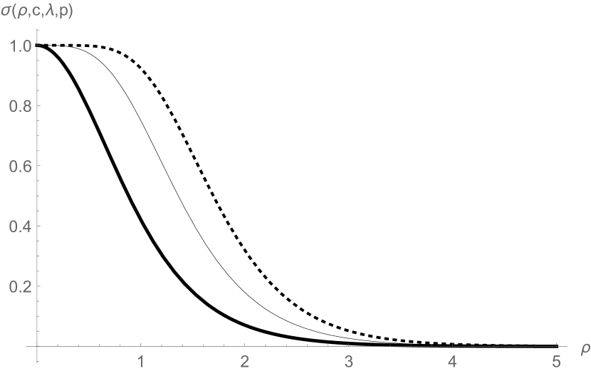
Figure 1: Warp factor for $p=1$ (thick line), $p=3$ (thin line) and $p=6$ (dotted line).

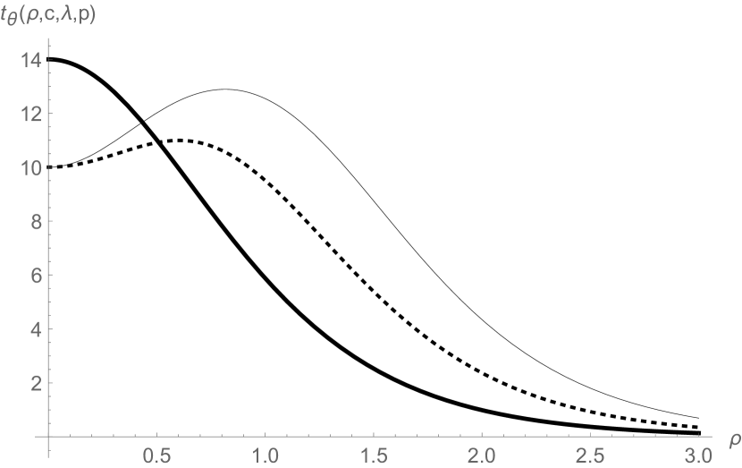
Figure 2: Angular pressure for $p=1$ (thick line), $p=3$ (thin line) and $p=6$ (dotted line).

The radial Einstein equation (7) provides a constraint between $A$ and $B$. Let us consider the ansatz for $B$ in the form

$$B(r)=A(r)+f(r).$$ (13)

For $f=0$ and $c=2\lambda$, the bulk metric has the form $ds^{2}=\text{sech}^{2}(\lambda r)\eta_{\mu\nu}dx^{\mu}dx^{\nu}+dr^{2}+R_{0}^{2}\text{sech}^{2}(\lambda r)d\theta^{2}$ Torrealba . Likewise the thin string-like model, this metric does not satisfy the condition expressed in Eq. (4), and then, at $r=0$, we have a 4-brane.

Since we seek for a regular geometry converging asymptotically to the $AdS_{6}$ spacetime and satisfying the regularity condition at the origin, let us adopt two models.

II.1 Warped disk

Consider $f_{1}(r):=\frac{m}{\lambda r}$. For this choice the metric has the form

$$ds^{2}=\sigma_{c,p,\lambda}(r)\eta_{\mu\nu}dx^{\mu}dx^{\nu}+dr^{2}+r^{m/\lambda}\sigma_{c,p,\lambda}(r)d\theta^{2}.$$ (14)

In order to satisfy the regularity conditions, we have to set $m=2\lambda$. Then, the metric (14) represents a warped product of the 3-brane and the two dimensional flat disk. The angular metric component is shown in Fig. 4 for $p=1$ where the high of the function increases with the ratio $c/\lambda$. Fig. 4 shows the Ricci scalar which for $p=1$ has a bell-shape and for $p=10$ exhibits a plateau near the origin. The components of the stress-energy tensor for $p=1$ are

$$t_{0}(r) = \kappa_{6}\left(\frac{(5c+4\lambda)}{2}\text{sech}^{2}(\lambda r)+\frac{5c}{2}\frac{\tanh(\lambda r)}{r}\right),$$

$$t_{r}(r) = \kappa_{6}\left(\frac{5c^{2}}{2}\text{sech}^{2}(\lambda r)+2c\frac{\tanh(\lambda r)}{r}\right).$$ (15)

We plotted these components for $c=2\lambda$ in Fig. 6. Note that the source of this geometry is localized around the origin and satisfies the dominant energy condition. For $p=6$, the core shows an internal structure where the peak of the components are shifted from the origin and the radial pressure is almost constant. The relationship between the bulk and brane Planck masses is given by

$$M_{4}^{2}=\frac{2\pi M_{6}^{4}}{\lambda}\int_{0}^{\infty}{r\text{sech}^{\frac{3c}{2\lambda}}{\lambda r}dr}.$$ (16)

For $c/\lambda=4/3$, we obtain $M_{4}^{2}=\frac{2\pi\ln{2}}{\lambda^{3}}M_{6}^{4}$. Then, the ratio $M_{4}/M_{6}$ increases as the brane width decreases.

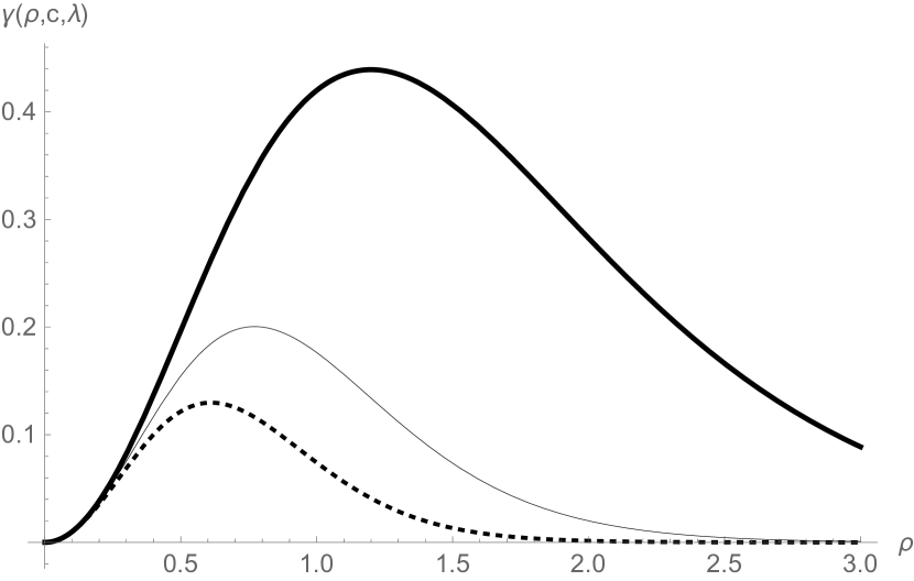
Figure 3: Angular metric component for $c/\lambda=2$ (thick line), $c/\lambda=4$ (thin line) and $c/\lambda=6$ (dotted line).

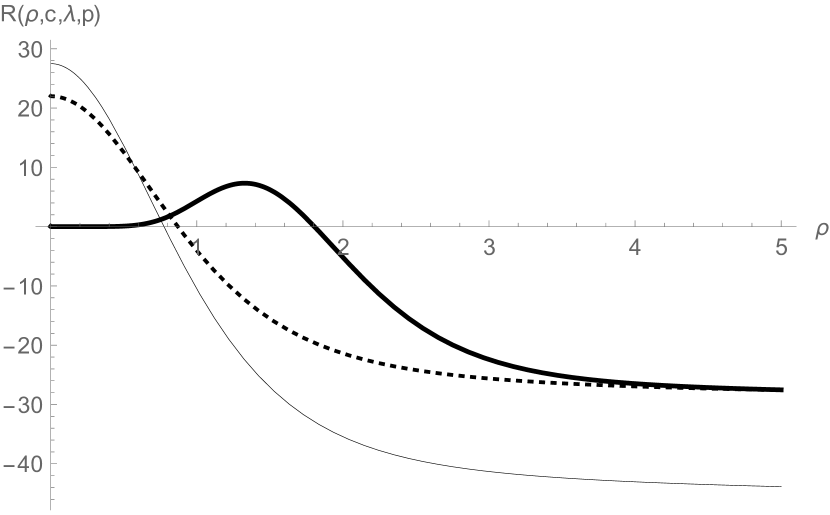
Figure 4: Ricci scalar for $p=1,c=2\lambda$ (dotted line), $p=1,c=2.5\lambda$ (thin line) and $c=2\lambda$ and $p=10$ (thick line).

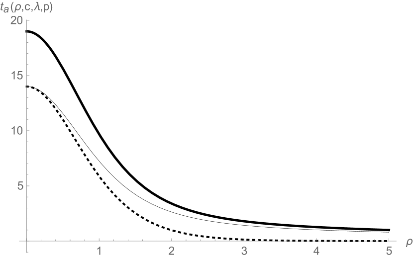
Figure 5: Energy density (thick line), radial pressure (thin line) and the angular pressure (dotted line) for $p=1$ and $c/\lambda=2$.

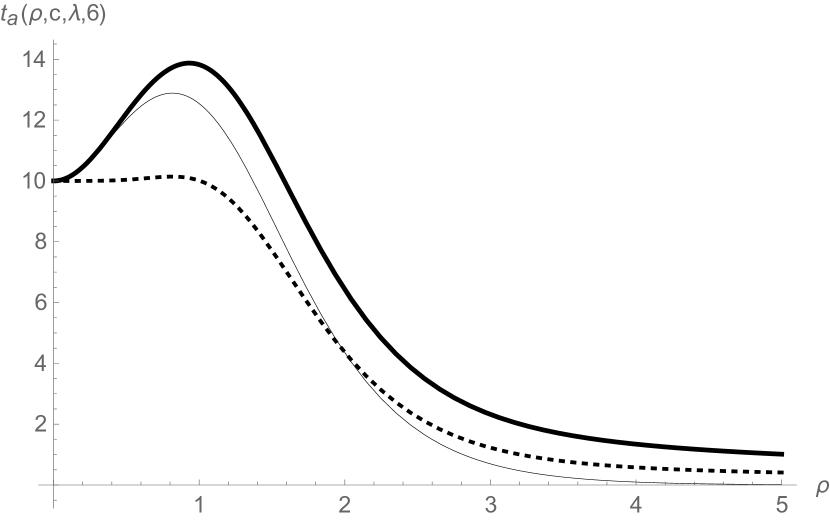
Figure 6: Energy density (thick line), radial pressure (dotted line) and the angular pressure (thin line) for $p=6$ and $c=2\lambda$.

II.2 Exotic string-brane

For $f(r)$ = $\frac{m}{\tanh(\lambda r)}$, the bulk metric has the form

$$ds^{2}=\text{sech}^{c/\lambda}(\lambda r)\eta_{\mu\nu}dx^{\mu}dx^{\nu}+dr^{2}+\frac{1}{\lambda^{\frac{m}{\lambda}}}\sinh^{\frac{m}{\lambda}}(\lambda r)\text{sech}^{c/\lambda}(\lambda r)d\theta^{2}.$$ (17)

The regularities conditions are satisfied for $m=2\lambda$. The components of the stress-energy tensor are

$$t_{0}(r) = \kappa_{6}\left(\frac{c(5c+4\lambda)}{2}\text{sech}^{2}(\lambda r)+\frac{\lambda(5c-2\lambda)}{2}\right),$$

$$t_{r}(r) = \kappa_{6}\left(\frac{5c^{2}}{2}\text{sech}^{2}(\lambda r)+2c\lambda\right),$$ (18)

whose are sketched in Fig. 8 for $c/\lambda=2$. The source satisfies the dominant energy condition inside the core and exhibits an exotic radial pressure asymptotically. For $c=\frac{2\lambda}{5}$, $t_{0}=t_{\theta}$ and the source is dominated by the radial pressure. Fig. 8 shows the behaviour of the Ricci scalar as we change the deformation parameter $p$. For $p=1$, the curvature smoothly goes to an asymptotic $AdS_{6}$ spacetime whereas for $p=10$ there is a $AdS_{6}$ plateau near the origin. In this scenario the bulk-brane relation mass is $M_{4}^{2}=\frac{4\pi}{(3c\lambda-2)\lambda^{2}}M_{6}^{4},$ which increases as the source width $\lambda$ decreases.

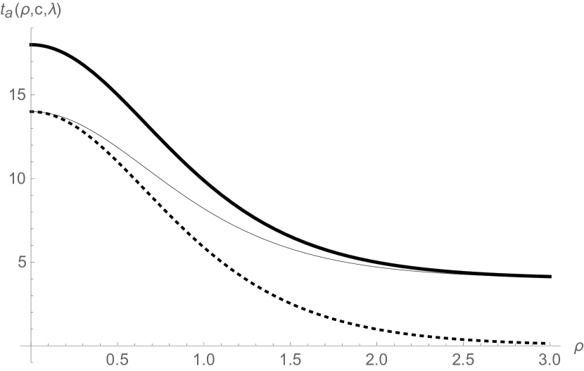
Figure 7: Energy density (thick line), radial pressure (thin line) and angular pressure (dotted line) for $p=\lambda=1,c=2$.

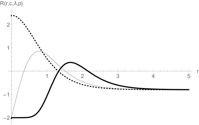
Figure 8: Ricci scalar for $c=\frac{2}{5},\lambda=1$ and $p=1$ (dotted line), $p=2$ (thin line), $p=10$ (thick line).

III Bosonic fields

In this section we study the effects of the warped disk and exotic string-like models have upon the gravitational, scalar and vector gauge fields.

III.1 Gravity perturbations

Assuming the metric perturbation $ds_{6}^{2}=\sigma(\eta_{\mu\nu}+h_{\mu\nu}(x^{\zeta},r,\theta,k)dx^{\mu}dx^{\nu}+dr^{2}+\gamma d\theta^{2}$, using the traceless transverse gauge $h_{\mu}^{\mu}=\nabla_{\mu}h^{\mu\nu}=0$ and performing the KK decomposition $h_{\mu\nu}(x^{\zeta},r,\theta)=\hat{h}_{\mu\nu}(x^{\zeta})\sum_{l=0}^{\infty}\chi(r)e^{il\theta},$ the linearized Einstein equation yields to the radial graviton equation resolvedconifold

$$\chi^{\prime\prime}_{g}(r)+\left(\frac{5}{2}\frac{\sigma^{\prime}}{\sigma}+\frac{1}{2}\frac{\beta^{\prime}}{\beta}\right)\chi^{\prime}_{g}(r)+\frac{1}{\sigma}\left(m^{2}-\frac{l^{2}}{\beta}\right)\chi_{g}(r)=0,$$ (19)

where $m$ is the KK mass satisfying $\Box_{4}\hat{h}_{\mu\nu}=-m^{2}\hat{h}_{\mu\nu}$ and $\beta=\gamma/\sigma$. For a factorizable Bulk, i.e., $\sigma=1$ and $\gamma=r^{2}$, the gravitational KK solutions are $\chi_{g}=c_{1}J_{l}(mr)+C_{2}Y_{l}(mr)$. Thus, for a noncompact extra dimension the massive KK modes form a tower of non-normalized states. For a compact transverse space, the asymptotic behaviour of the massive spectrum is $m_{n}\approx n\pi/R$. The warped scenarios bring a strong dependence of the cosmological constant and the brane source upon the KK modes, as we show in next sections.

III.2 Scalar field

Consider a minimally coupled massless scalar field $\Phi$ whose bulk action is given by

$$S_{\Phi}=-\frac{1}{2}\int{g^{MN}\nabla_{M}\Phi\nabla_{N}\Phi\sqrt{-G}d^{6}x}.$$ (20)

The Bulk scalar field satisfies the equation of motion (EoM)

$$\frac{1}{\sqrt{-G}}\partial_{M}(\sqrt{-G}g^{MN}\partial_{N}\Phi)=0,$$ (21)

which after the Kaluza-Klein (KK) reduction $\Phi(x^{\mu},r,\theta)=\hat{\Phi}(x^{\mu})\sum_{l}{\chi_{s}(r)e^{il\theta}}$ yields to

$$\chi_{s}^{\prime\prime}(r)+\left(\frac{5}{2}\frac{\sigma^{\prime}}{\sigma}+\frac{1}{2}\frac{\beta^{\prime}}{\beta}\right)\chi_{s}^{\prime}(r)+\frac{1}{\sigma}\left(m^{2}-\frac{l^{2}}{\beta}\right)\chi_{s}(r)=0.$$ (22)

It is worthwhile to stress that the graviton eq. (19) has the same form of the radial equation for a massless scalar field (22). Accordingly, hereinafter we shall concern ourselves to the graviton radial function and the results extend to the scalar field straightforward.

III.3 Vector field

For the vector gauge field we assume a Maxwell action on the Bulk in the form

$$S_{A}=-\frac{1}{4}\int{g^{MR}g^{NS}F_{MN}F_{RS}\sqrt{-G}d^{6}x},$$ (23)

where $F_{MN}:=\partial_{[M}A_{N]}$. Thus, the Bulk photon obeys the equation $\partial_{M}(\sqrt{-G}F^{MN})=0$ and assuming the gauge $\partial_{\mu}A^{\mu}=A_{\theta}=0$, the radial function $\chi_{A}(r)$ of the Kaluza-Klein decomposition $A_{\mu}(x^{M})=\sum_{l=0}^{\infty}A_{\mu}^{(l)}(x^{\mu})\chi_{A}(r)Y_{l}(\theta)$ for $l=0$ satisfies gaugecigar

$$\chi^{\prime\prime}_{A}(r)+\left(\frac{3}{2}\frac{\sigma^{\prime}}{\sigma}+\frac{1}{2}\frac{{\beta}^{\prime}}{\beta}\right)\chi^{\prime}_{A}(r)+\frac{m^{2}}{\sigma}\chi_{A}(r)=0.$$ (24)

It is worthwhile to stress the resemblance among the gravitational (scalar) and the gauge radial equations. In fact, for $l=0$, it is possible to unify these equation as

$$y^{\prime\prime}_{q}(r)+\left(\frac{q}{2}\frac{\sigma^{\prime}}{\sigma}+\frac{1}{2}\frac{{\beta}^{\prime}}{\beta}\right)y^{\prime}_{q}(r)+\frac{m^{2}}{\sigma}y_{q}(r)=0,$$ (25)

where $q=5$ for the gravitational and scalar fields and $q=3$ for the gauge vector field. In the following, we use the compact form in Eq.(25) in order to compare the properties among the bosonic fields.

III.4 Massless modes

For $m=0$ (massless KK mode) and $l=0$ (s-state), the only normalizable solutions are the constants $\chi_{g0}=\chi_{s0}=N_{g}$ and $\chi_{A0}=N_{A}$. In the conformal variable $z=\int_{0}^{r}\sigma^{-\frac{1}{2}}dr^{\prime}$, these gravitational (scalar) and gauge normalizable massless modes can be rewritten as

$$\Psi_{0g} = N_{g}\sigma\beta^{\frac{1}{4}},$$ (26)

$$\Psi_{0A} = N_{A}\sigma^{\frac{1}{2}}\beta^{\frac{1}{4}}.$$ (27)

For $c=2\lambda$, the conformal variable is given by $z=\sinh(\lambda r)/\lambda$ whereas for $c=6\lambda$, $z=(9\sinh(\lambda r)+\sinh(3\lambda r))/12$. For the warped disk model and $c=2\lambda$, the warp factor has the form $\sigma(z)=1/(1+\lambda^{2}z^{2})$ and $\beta(z)=(\sinh^{-1}{\lambda z})^{2}/\lambda^{2}$. We plotted the graviton (scalar) and photon massless modes for $\lambda=1$ in Fig. (10) and in Fig. (10). Note that even though the massless modes are constant in the radial coordinate they exhibit a normalized profile in the conformal coordinate. The asymptotic exponential behaviour reflects the $AdS$ regime similar to the thin string-like scenarios Gherghetta . The divergence near the origin stems from the change to the conformal coordinate.

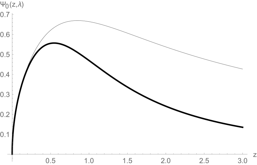
Figure 9: Gravitational (thick line) and vector gauge (thin line) massless modes for $l=0$ in the warped disk model $(c=2\lambda)$.

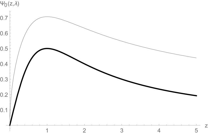
Figure 10: Gravitational (thick line) and vector gauge (thin line) massless modes for $l=0$ in the exotic string model $(c=2\lambda)$.

III.5 Massive modes

For $m\neq 0$, the KK radial equation in the warped disk model becomes

$$y_{m,l,q}^{{}^{\prime\prime}}+\left(\frac{1}{r}-\frac{qc}{2}\tanh(\lambda r)\right)y_{m,l,q}^{{}^{\prime}}+\cosh(\lambda r)^{c/\lambda}\left(m^{2}-\frac{l^{2}}{r^{2}}\right)y_{m,l,q}=0,$$ (28)

where $q=5$ for the graviton (and the scalar field) and $q=3$ for the photon. Near the brane, by expanding Eq.(28) up to first order, we obtain

$$y_{m,l,q}^{{}^{\prime\prime}}+\left(\frac{1}{r}-\frac{qc\lambda r}{2}\right)y_{m,l,q}^{{}^{\prime}}+\left(m^{2}-\frac{l^{2}}{r^{2}}\right)y_{m,l,q}=0,$$ (29)

whose solutions are

$$y_{m,l,q}(r)=A_{m,l,q}\sum_{k=0}^{\infty}{\Big{[}\frac{\left(qc\lambda l-2m^{2}\right)^{k}}{m^{2k}(2k)!}+(qc\lambda)^{k}\Big{]}\frac{(mr)^{2k+l}}{2^{2k}(l)_{k}}},$$ (30)

where $A_{m,l,q}$ is an integration constant. The KK modes have a zero of order $l$ at the origin. Then, for $l=0$, $y_{m,0,q}(r)\rightarrow A_{m,l,q}$ as $r\rightarrow 0$, whereas for $l\neq 0$, $y_{m,l,q}(r)\rightarrow 0$. For $r<<\sqrt{2/qc\lambda}$ the KK modes are described by $y_{m,l,q}(r)=A_{m,l,q}J_{l}(mr)$. Hence, only the s-wave $l=0$ state is allowed on the brane. Asymptotically, Eq.(28) becomes the thin string-like equation $y_{m,l,q}^{{}^{\prime\prime}}-\frac{qc}{2}y_{m,l,q}^{{}^{\prime}}+m^{2}\frac{e^{cr}}{2^{c/\lambda}}y_{m,l,q}=0,$ whose solution is Gherghetta :

$$y_{q,m,l}(r)=e^{\frac{qcr}{4}}\left(A_{1}J_{q/2}\left(\frac{2^{\frac{2\lambda-c}{2\lambda}}me^{\frac{cr}{2}}}{c}\right)+A_{2}Y_{q/2}\left(\frac{2^{\frac{2\lambda-c}{2\lambda}}me^{\frac{cr}{2}}}{c}\right)\right).$$ (31)

For the exotic string model, the KK tower satisfies

$$y_{m,l,q}^{{}^{\prime\prime}}+\left(\lambda\coth(\lambda r)-\frac{qc}{2}\tanh(\lambda r)\right)y_{m,l,q}^{{}^{\prime}}+\cosh(\lambda r)^{c/\lambda}\left(m^{2}-\frac{(l\lambda)^{2}}{\sinh^{2}(\lambda r)}\right)y_{m,l,q}=0,$$ (32)

which has the same near brane behavior of the warped disk model. However, far from the brane the KK eigenfunctions are given by

$$y_{q,m,l}(r)=e^{\frac{(qc-2\lambda)r}{4}}\left(A_{1}J_{(qc-2\lambda)/2c}\left(\frac{2^{\frac{2\lambda-c}{2\lambda}}me^{\frac{cr}{2}}}{c}\right)+A_{2}Y_{(qc-2\lambda)/2c}\left(\frac{2^{\frac{2\lambda-c}{2\lambda}}me^{\frac{cr}{2}}}{c}\right)\right).$$ (33)

The presence of the width brane parameter $\lambda$ shows that the exotic source modifies the KK tower even outside the brane core.

Unlike the massless modes, the massive states forms a tower of non-normalizable states. Important qualitative features about the massive spectrum, as its stability and mass gap, can be obtained from the analogue Schrödinger potential. In the conformal coordinate $z=\int_{0}^{r}\sigma^{-\frac{1}{2}}dr^{\prime}$ and defining $\Psi_{g}=\sigma\beta^{\frac{1}{4}}\chi$ and $\Psi_{A}=\sigma^{\frac{1}{2}}\zeta^{\frac{1}{4}}$, we transform the Eq. (19) and Eq. (24) into a Schrödinger-like equation Dantas

$$-\ddot{\Psi}(z)+U(z)\Psi(z)=m^{2}\Psi(z),$$ (34)

where $U_{g}(z)=\dot{W}_{g}(z)+W_{g}^{2}+\frac{l^{2}}{\beta}$, and $U_{A}(z)=\dot{W}_{A}(z)+W_{A}^{2}$ are the analogue Schrödinger potential and $W_{g}(z)=\frac{\dot{\sigma}}{\sigma}+\frac{1}{4}\frac{\dot{\beta}}{\beta}$, and $W_{A}(z)=\frac{1}{2}\frac{\dot{\sigma}}{\sigma}+\frac{1}{4}\frac{\dot{\beta}}{\beta}$ are the respective gravitational and gauge super potential Dantas . The existence of such super potentials guarantees the absence of tachyonic (unstable) massive states Dantas .

We plotted the graviton Schrödinger potential for the warped disk in Fig. 12 and for the exotic string in Fig. 12. Since asymptotically both potentials vanish, the massive modes are gappless free states. The scalar and vector gauge potentials have similar behavior.

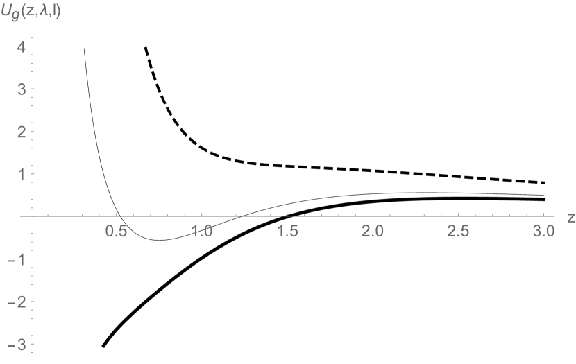
Figure 11: Gravitational (and scalar field) Schrödinger potential in the warped disk model for $\lambda=0.3$ and $c=0.6$. Thick line $l=0$, thin line $l=1$ and dashed line $l=2$.

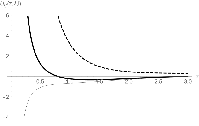
Figure 12: Gravitational (and scalar field) Schrödinger potential in the exotic string model for $\lambda=0.1)$ and $c=0.6$. Thin line $(l=0)$, thick line $(l=1)$ and dashed line $l=2$.

The potential exhibits an infinite well at the origin for $l=0$ and an infinite barrier for $l\neq 0$. Then, only the $l=0$ states are allowed at the brane, as previously discussed. For $l=1$, it turns out that the potential has a finite well displayed from the origin, where resonant massive KK gravitons can be found.

IV Conclusions and perspectives

We proposed a new class of smooth thick string-like model with an $AdS_{6}$ asymptotic regime. A localized and bell-shaped source satisfying the dominant energy condition was found, where the properties of the source and the geometry are dependent on the ratio between the cosmological constant and the brane width. A richer internal brane structure can be introduced by means of a varying brane-tension, which modifies how the curvature and the energy density vary inside the brane core. Amidst the thick string-like branes found, a bell-shaped source satisfying the dominant energy condition shares a great resemblance with the numerical Abelian vortex brane (Giovannini, ).

The scalar, gravitational and vector gauge sectors were also analysed. They showed similar features, as normalizable massless Kaluza-Klein modes and an attractive potential for the massive KK tower at the origin for the $l=0$ states. For $l\neq 0$, the infinite barrier at the origin avoids the detection of these modes at the brane. Nevertheless, for $l=1$, we found a potential well besides the origin, where massive resonant states could be detected.

As perspectives, we point out the use of numerical analysis to deduce these geometrical solutions from a Lagrangian model, such as a deformed Abelian vortex Giovannini . For the KK spectrum and its phenomenological consequences, as the correction to the Newtonian and Coulomb potentials, numerical methods should also be carried out. We expect a strong influence of the brane width parameter and the bulk cosmological constant on the KK spectrum. The behavior of the massless mode and divergence the Schrödinger potential near the brane suggests the inclusion of an interaction term between the fields and the brane, as performed in the DGP models Dvali .

References

- (1) L. Randall and R. Sundrum, Phys. Rev. Lett. 83, 3370 (1999).
- (2) L. Randall and R. Sundrum, Phys. Rev. Lett. 83, 4690 (1999).
- (3) C. Csaki, M. Graesser, L. Randall and J. Terning, Phys. Rev. D 62, 045015 (2000).
- (4) T. Gherghetta and B. von Harling, JHEP 1004, 039 (2010).
- (5) A. Kehagias and K. Tamvakis, Phys. Lett. B 504, 38 (2001).
- (6) D. Bazeia and A. R. Gomes, JHEP 0405, 012 (2004).
- (7) O. DeWolfe, D. Z. Freedman, S. S. Gubser and A. Karch, Phys. Rev. D 62, 046008 (2000).
- (8) Martin Gremm, Phys. Lett. B 478, 434-438 (2000).
- (9) C. Csaki, J. Erlich, and T. J. Hollowood, Phys. Rev. Lett. 84, 5932 (2000).
- (10) I. Olasagasti and A. Vilenkin, Phys. Rev. D 62, 044014 (2000).
- (11) R. Gregory, Phys. Rev. Lett. 84, 2564 (2000).
- (12) T. Gherghetta and M. E. Shaposhnikov, Phys. Rev. Lett. 85, 240 (2000).
- (13) A. Kehagias, Phys. Lett. B 600, 133 (2004).
- (14) A. G. Cohen and D. B. Kaplan, Phys. Lett. B 470, 52 (1999).
- (15) M. Giovannini, H. Meyer and M. E. Shaposhnikov, Nucl. Phys. B 619, 615 (2001).
- (16) Y. Brihaye, T. Delsate, N. Sawado and Y. Kodama, Phys. Rev. D 82, 106002 (2010).
- (17) I. Oda, Phys. Rev. D 62 126009 (2000).
- (18) I. Oda, Phys. Lett. B 496, 113 (2000).
- (19) Y. -X. Liu, L. Zhao and Y. -S. Duan, JHEP 0704, 097 (2007).
- (20) P. Tinyakov and K. Zuleta, Phys. Rev. D 64, 025022 (2001).
- (21) B. de Carlos and J. M. Moreno, JHEP 0311, 040 (2003).
- (22) J. E. G. Silva, V. Santos, C. A. S. Almeida, Class. Quant. Grav. 30, 025005 (2013).
- (23) J. E. G. Silva and C. A. S. Almeida, Phys. Rev. D 84, 085027 (2011).
- (24) R. S. Torrealba, Phys. Rev. D 82, 024034 (2010).
- (25) M. Gogberashvili, P. Midodashvili and D. Singleton, JHEP 0708, 033 (2007).
- (26) Y. -S. Duan, Y. -X. Liu and Y. -Q. Wang, Mod. Phys. Lett. A 21, 2019 (2006).
- (27) F. W. V. Costa, J. E. G. Silva and C. A. S. Almeida, Phys. Rev. D 87, 125010 (2013).
- (28) D. M. Dantas, D. F. S. Veras, J. E. G. Silva and C. A. S. Almeida, Phys. Rev. D 92, 10, 104007 (2015).
- (29) G. R. Dvali, G. Gabadadze and M. Porrati, Phys. Lett. B 485, 208 (2000).