The Interplay of Structure and Dynamics in the Raman Spectrum of Liquid Water over the Full Frequency and Temperature Range

Tobias Morawietz Department of Chemistry, Stanford University, Stanford, CA 94305, United States Ondrej Marsalek Faculty of Mathematics and Physics, Charles University, Ke Karlovu 3, 121 16 Prague 2, Czech Republic Shannon R. Pattenaude Department of Chemistry, Purdue University, West Lafayette, IN 47907, United States Louis M. Streacker Department of Chemistry, Purdue University, West Lafayette, IN 47907, United States Dor Ben-Amotz Department of Chemistry, Purdue University, West Lafayette, IN 47907, United States Thomas E. Markland tmarkland@stanford.edu Department of Chemistry, Stanford University, Stanford, CA 94305, United States

Abstract

While many vibrational Raman spectroscopy studies of liquid water have investigated the temperature dependence of the high-frequency O-H stretching region, few have analyzed the changes in the Raman spectrum as a function of temperature over the entire spectral range. Here, we obtain the Raman spectra of water from its melting to boiling point, both experimentally and from simulations using an ab initio-trained machine learning potential. We use these to assign the Raman bands and show that the entire spectrum can be well described as a combination of two temperature-independent spectra. We then assess which spectral regions exhibit strong dependence on the local tetrahedral order in the liquid. Further, this work demonstrates that changes in this structural parameter can be used to elucidate the temperature dependence of the Raman spectrum of liquid water and provides a guide to the Raman features that signal water ordering in more complex aqueous systems.

TOC graphic

I Introduction

Despite the importance of liquid water and the structural and dynamic sensitivity of vibrational Raman spectroscopy, quantitatively linking water spectra and structure remains a challenge for experiment and theory.Bakker and Skinner (2010) Indeed, few experimental studies have spanned the entire liquid temperature and vibrational frequency range: from the low frequency intermolecular hydrogen bond (H-bond) stretch, O-H…O at $\sim$ 180 cm^-1, to the high-frequency O-H stretch region at $\sim$ 3400 cm^-1.Scherer et al. (1974); Zhelyaskov et al. (1989); Bray et al. (2013); De Santis et al. (1987); Walrafen (1974); Murphy and Bernstein (1972); Hare and Sorensen (1990); Walrafen et al. (1986a) The need for such experimental results is particularly timely as it is becoming increasingly practical to simulate the Raman spectra of water using first principles approaches across the entire frequency range,Wan et al. (2013); Medders and Paesani (2015); Marsalek and Markland (2017) thus providing a strenuous test of these methods’ ability to correctly capture and elucidate the structure and dynamics of water. Here we employ a combined experimental and theoretical strategy to address the open questions regarding the origin of vibrational features in the Raman spectra of liquid water from its melting to boiling point.

Many previous experimental Raman studiesScherer et al. (1974); Hare and Sorensen (1990); Walrafen et al. (1986a); D’Arrigo et al. (1981); Walrafen et al. (1986b); Sun (2013) have concentrated on analyzing the temperature dependence of the O-H stretching region where an isosbestic point, a region in the spectrum where the intensity is approximately constant upon a change in temperature,Walrafen et al. (1986b) is observed. The bimodal profile of the isotropic line shape together with the observation of an isosbestic point has been frequently attributed to an equilibrium between O-H bonds that correspond to water molecules in two different local environments.Walrafen et al. (1986a); D’Arrigo et al. (1981); Sun (2013); Harada et al. (2017) Although such isosbestic behavior is expected for spectra composed of two components, it can also arise from a continuous distribution of thermally equilibrated structures.Geissler (2005); Smith et al. (2005) Theoretical studies have thus sought to simulate and decompose the Raman spectra. For example the temperature dependence of the isotropic Raman O-H stretching band has been shown to be remarkably well reproduced by simulations employing rigid water models using mappings between the vibrational frequency and the local electric fieldCorcelli et al. (2004); Corcelli and Skinner (2005); Auer and Skinner (2008); Yang and Skinner (2010); Tainter et al. (2013) while some early studies have calculated the low frequency terahertz region from time-correlation functions of the polarizability tensor.Madden and Impey (1986); Mazzacurati et al. (1989); Bursulaya and Kim (1998) However, more recently it has become possible to use high-level ab initio-based potential energy surfacesMedders and Paesani (2015) or ab initio molecular dynamics (AIMD) calculations with classicalWan et al. (2013); Marsalek and Markland (2017) and even quantum nucleiMarsalek and Markland (2017) to make fully first principles predictions of the Raman spectrum at ambient conditions across the entire frequency range.

Here we present a combined experimental and theoretical study of the temperature- dependent Raman spectra of liquid water from its freezing to boiling point over the full frequency range, from $\sim$ 100 cm^-1 to $\sim$ 4200 cm^-1. By doing this we address open questions regarding the origin of vibrational features that are more prominent in the Raman than Infrared (IR) spectra and the correlation between the vibrational and structural properties of water. To increase the efficiency of our simulations we employ neural network potentials (NNPs)Behler and Parrinello (2007); Artrith and Urban (2016); Behler (2016); Morawietz et al. (2016) trained to density functional theory calculations (see Supporting Information (SI), sections 1-3). By experimentally and theoretically probing the entire vibrational frequency range here we provide a rigorous assignment of the low-intensity modes in the vibrational spectra and identify several spectral regions, in addition to the O-H stretching region, that exhibit strong dependence on the local tetrahedral order of the liquid. Our results further reveal that the temperature dependence of both the vibrational spectrum of water and its tetrahedral order distribution can be accurately decomposed into a linear combination of two temperature-independent components. By employing a time-dependent analysis of our simulated spectra, we provide theoretical support for the empirical observation that enhanced tetrahedral order is associated with features appearing across the entire frequency range, from the low-frequency H-bond stretch band to the high-frequency O-H stretch band. This analysis allows us to identify the regions that provide the most sensitive spectral signatures of structural ordering in liquid water, thus offering insights into the origins of these features. The identification of these features will aid in the analysis of other complex aqueous environments ranging from the hydration-shells of solute molecules to catalytic surfaces and biological interfaces.Heyden et al. (2008); Artrith and Kolpak (2014); Gierszal et al. (2011); Fayer and Levinger (2010); Crans and Levinger (2012); Davis et al. (2012); Bakulin et al. (2013); Russo et al. (2017)

II Results and Discussion

Refer to caption — Figure 1: Comparison of the experimental and simulated anisotropic and isotropic reduced Raman spectra (a-d) and the simulated hydrogen vibrational density of states (VDOS, shown on a logarithmic scale to highlight the low-intensity features) (e) of liquid water at different temperatures. For clarity, the low frequency region was scaled by the factor indicated in the plot. All spectra are truncated at 100 cm^-1 which is the lowest frequency for which accurate experimental intensities were obtained. All spectra are normalized to unit area. The standard deviation $\sigma$ , with respect to temperature (shown as grey shading), was used to locate isosbestic points which are depicted as blue lines. The hydrogen VDOS spectrum can be divided into four regions, each of which has an isosbestic point at the center and is separated by isosbestic points from the other regions.

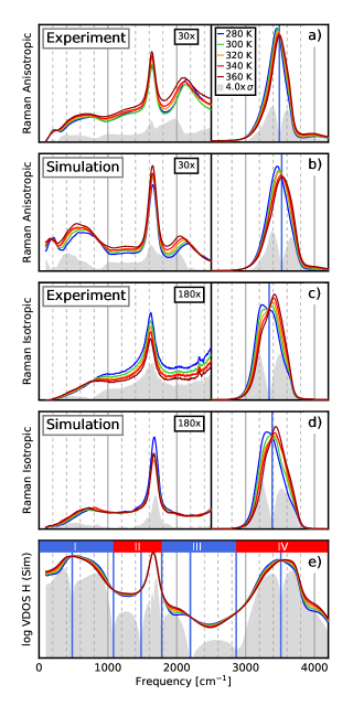
In Fig. 1 we compare the experimental (panels a and c) and simulated (panels b and d) anisotropic and isotropic Raman spectra of liquid water. The spectra are presented in a reduced formBrooker et al. (1988, 1989) (see SI sections 4-5) that is particularly useful for such a comparison, as it highlights features in the low frequency region, and removes the dependence on the incident laser frequency. Fig. 1e shows the temperature-dependent vibrational density of states (VDOS) of the hydrogen atoms (on a logarithmic-scale for better visibility of the low-intensity regions) which exhibits analogous trends to those seen in the Raman spectra. The low-frequency band at $\sim$ 200 cm^-1, which has been attributed to the (intermolecular) H-bond stretching mode,Walrafen et al. (1986a) is barely visible in the hydrogen VDOS, but is more prominent in the oxygen VDOS (see SI section 6). The grey shading in Fig. 1 shows the standard deviation of the spectral data obtained at different temperatures and thus gives an indication of the temperature sensitivity of different spectral regions. The minima in the standard deviation thus allow for the approximate identification of isosbestic points (frequencies where the spectral intensity is temperature- independent).

The high-frequency O-H stretching region (from $\sim$ 2500 cm^-1 to $\sim$ 4200 cm^-1) of the anisotropic and isotropic Raman spectra has been the focus of the majority of previous studies.Scherer et al. (1974); Hare and Sorensen (1990); Walrafen et al. (1986a); D’Arrigo et al. (1981); Walrafen et al. (1986b); Sun (2013); Harada et al. (2017); Corcelli et al. (2004); Corcelli and Skinner (2005); Auer and Skinner (2008); Tainter et al. (2013) As observed in Fig. 1a, the anisotropic O-H band consists of a single peak that decreases in intensity and shifts to higher frequencies as the temperature is raised, which resembles the behavior seen in the IR spectrum of liquid water,Maréchal (2011) while the isotropic band has a bimodal profile (Fig. 1c). A feature that is not evident in the IR spectrum but appears in the anisotropic Raman spectrum is the high-frequency band at around 4000 cm^-1, which is higher than even the O-H stretch frequency of the isolated molecule ( $\sim$ 3750 cm^-1). To identify the origin of this feature, which is observed both in our experiments and simulations, we show the synchronous two-dimensional (2D) correlation spectrumNoda (1993) of the simulated VDOS in Fig. 2a (also see SI section 7). This analysis indicates the frequencies that are positively correlated (red regions) and those that are anticorrelated (blue regions) and thus allows us to identify the vibrational modes with which the high-frequency feature is correlated. As seen in Fig. 2b, the 4100 cm^-1 band is strongly correlated with two bands at lower frequencies – one with its maximum in the libration region (centered at 433 cm^-1) and one in the O-H stretch region (centered at 3645 cm^-1) – whose sum yields a combined frequency of 4078 cm^-1. The fact that this mode is strongly associated with two bands that sum to give its frequency supports an assignment of this feature as a combination band (i.e. arising from anharmonic couplings of two or more fundamental modes at frequencies slightly lower than the sum of the fundamental frequencies). This is in contrast with a previous assignmentWalrafen and Pugh (2004) that, while identifying the 4100 cm^-1 band as arising from librational-vibrational coupling, assigned it as a combination of a higher frequency librational band (730 cm^-1) with the low frequency part of the stretch (3423 cm^-1), whereas our simulations suggest it arises from coupling between a higher frequency part of the O-H stretch and a lower frequency librational band.

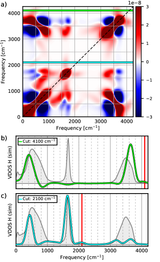
In the low-frequency region of the spectrum, we observe a broad feature centered at 2100 cm^-1 (sometimes referred to as the water association band), which is visible in both the experimental and calculated anisotropic Raman spectra. Interestingly, this band at 2100 cm^-1 was not present in recent anisotropic Raman spectra calculated using the ab initio-based MB-pol model. 11 Experimental and theoretical studies of the IR spectra of liquid water, ice, and trehalose-water systems have previously assigned this feature to a combination band of the bending mode with a librational modeMaréchal (1991); McCoy (2014) or, alternatively, to the second overtone of a librational mode.Devlin et al. (2001) Our 2D correlation analysis of our NNP simulations (see Fig. 2c) shows that the 2100 cm^-1 band is a combination band of the low-frequency libration band (centered at 433 cm^-1) with the bend vibration (centered at 1631 cm^-1) summing to a frequency of 2064 cm^-1.

The agreement between our measured and simulated Raman spectra in the O-H stretching region is markedly better than that observed in another recent AIMD simulation, using a different exchange-correlation functional, where the O-H stretching band was red-shifted by 200 cm^-1and significantly broadened compared to the experiment.Wan et al. (2013) The location of the isosbestic points in the O-H stretch region are also well reproduced by our simulations (3532 cm^-1 for the anisotropic spectrum and 3385 cm^-1 for the isotropic one compared to 3490 cm^-1 and 3330 cm^-1 in the experiment). While the overall shape of the simulated anisotropic spectra in the low frequency region deviates slightly from the measured spectra, the position and shape of the individual spectral features and their variation with temperature closely match those seen in the experiment. Having confirmed the agreement between our ab initio-based NNP simulations and the experimental Raman spectra over the full liquid temperature range, we can now use the simulations to relate the observed spectral features to the structural environments in the liquid.

What are the structural changes that lead to the temperature dependence of the different vibrational features occurring across the full frequency range of the Raman spectra? To begin to investigate this question, we first performed a self-modeling curve resolution (SMCR)Lawton and Sylvestre (1971); Tauler et al. (1995); Jiang et al. (2004) decomposition of the temperature-dependent vibrational spectra obtained from experiment and simulation. SMCR provides a means of decomposing a collection of two or more spectra into a linear combination of different spectral components, each of which has exclusively positive intensity. For example, SMCR has been used to separate aqueous solution spectra into a linear combination of bulk water and a solute-correlated component to reveal features arising from water molecules that are perturbed by solutes, including ions,Daly Jr. et al. (2017); Rankin and Ben-Amotz (2013) gases,Zukowski et al. (2017) alcohols,Davis et al. (2012); Rankin et al. (2015); Mochizuki et al. (2016) aromatics,Gierszal et al. (2011); Scheu et al. (2014) surfactants,Long et al. (2015); Pattenaude et al. (2016) and polymers.Mochizuki and Ben-Amotz (2017) Here, we employ an SMCR analysis to assess how accurately the temperature-dependent vibrational spectra can be approximated by a linear combination of two components, whose relative populations, but not spectral shapes, change with temperature.

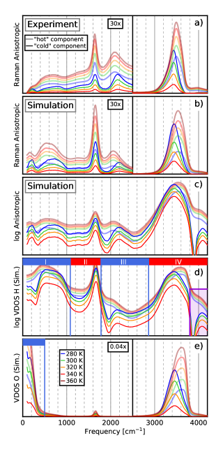
Fig. 3 shows the SMCR decomposition of our experimental and simulated anisotropic Raman spectra as well as the simulated VDOS spectra, which yields a high-temperature “hot” component, closely resembling the full spectrum at 360 K, and a “cold” component, whose intensity increases at low temperatures and whose spectral features are shifted relative to the “hot” component. As shown in SI Figs. S6 and S7, the reconstructed spectra, obtained by combining the two temperature-independent “hot” and “cold” components weighted by their populations, are almost indistinguishable from the original spectra and exhibit integrated fractional errors below 0.01 (see SI section 8) suggesting that the vibrational spectra of water can be accurately represented as a linear combination of two temperature-independent components over its entire liquid temperature range.

By inspecting the two components we observe that, for the “cold” component, the libration band and the combination band at 2100 cm^-1 are shifted to higher frequencies, and that a high-frequency peak centered at $\sim$ 4100 cm^-1 appears. The most prominent bands in the low temperature SMCR-spectra are peaked near $\sim$ 200 cm^-1 and 3400 cm^-1 and resemble those observed in ice and solid clathrate hydrates. Specifically, H₂O ice contains prominent bands at $\sim$ 180 cm^-1 and $\sim$ 3100 cm^-1.Davis et al. (2012); Kanno et al. (1998) Similarly, the Raman spectra of various H₂O clathrate hydrates contain bands peaked near $\sim$ 210 cm^-1 and $\sim$ 3100 cm^-1.Takasu et al. (2003); Sugahara et al. (2005); Chazallon et al. (2007) The similar positions of the bands in these tetrahedrally ordered phases to those seen in the SMCR decomposition of the liquid water spectra suggests that these bands may provide spectroscopic probes of the local tetrahedral order in the liquid. We note that even though the band at $\sim$ 200 cm^-1 is barely visible in the SMCR decomposed hydrogen VDOS, it can be seen much more prominently in the oxygen VDOS. This behavior is in-line with isotope substitution studies that find larger isotope shifts of this band in the Raman spectrum for a ¹⁶O/¹⁸O substitution compared to a H/D substitution, suggesting that it arises primarily from oxygen motions, consistent with the assignment of this band to the O-H…O H-bond stretch vibration.Brooker et al. (1989)

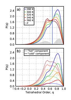
Given the good agreement with the experiment, we now use our simulations to assess whether the tetrahedral order in the liquid is indeed the cause of the observed spectral shifts by analyzing the temperature dependence of the local tetrahedral order parameterChau and Hardwick (1998) in its rescaled version 64 (such that it gives a value of 1 for a regular tetrahedron and averages to 0 for an ideal gas). The local tetrahedral order parameter (or tetrahedrality), $q_{i}$ , is a measure for the local angular order of water molecule i, based on its four nearest neighbors. The tetrahedrality distribution computed from our simulations (Fig. 4a), shows the bimodal structure seen in many previous simulations of liquid water,Russo et al. (2017); Errington and Debenedetti (2001); Paolantoni et al. (2009) with an isosbestic point at $q\approx$ 0.67. Upon cooling the distribution shifts to the right, indicating the more predominantly tetrahedral character expected at lower temperatures. To relate the vibrational spectra to the tetrahedrality of the liquid we perform an SMCR decomposition of the tetrahedral order parameter, shown in Fig. 4b, analogous to the decomposition of the vibrational spectra. From this we see that, like the spectra, the tetrahedral order distribution can be accurately decomposed into two temperature-independent components. The low-temperature component is shifted to high values of q and the broader high-temperature component is centered at lower q values. While these results demonstrate that the vibrational shifts and the tetrahedrality of the liquid exhibit similar temperature dependence, they alone do not provide direct proof that the spectral shifts are caused by the tetrahedrality of the environment.

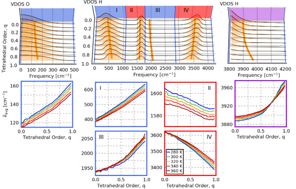
To establish the explicit connection between the spectral contribution of a water molecule in the liquid and its tetrahedral order we thus performed a time-dependent analysis of our simulated spectra.Marsalek and Markland (2017); Napoli et al. (2017) These results are shown in Fig. 5, where the contribution of a given molecule to the vibrational spectrum at a specific point in time is correlated with the instantaneous tetrahedrality of the local hydrogen environment of the same water molecule. For this analysis we employ the VDOS to extract the vibrational motions of individual atoms. The top panels in Fig. 2 show results obtained from the VDOS spectra at 320 K, binned as a function of the tetrahedrality parameter over the full frequency range. The bottom panels show how the average frequency in six regions of the spectrum changes with the local tetrahedral order of the water molecule. Four of these spectral regions were defined using the seven isosbestic points, identified from the temperature-dependent VDOS (regions I – IV, defined in Fig. 1e). The other two were chosen to be the 4000 cm^-1combination band identified earlier (defined in Figure 3d) and the 200 cm^-1O-H…O H-bond stretch vibration in the oxygen VDOS (Fig. 3e).

The results in Fig. 5 (bottom panels) demonstrate that there is a direct correlation between vibrational frequency and tetrahedrality in all spectral regions: in some regions the spectrum shifts to higher frequencies as the tetrahedrality increases while in others it shifts to lower frequencies. The O-H stretching band (region IV) is inversely correlated with the tetrahedral order, while the low frequency H-bond stretching band (oxygen VDOS), the libration band (region I), the combination band at 2100 cm^-1 (region III), and the high-frequency combination band near 4000 cm^-1, all are positively correlated. We observe that the bend (region II) displays the least sensitivity with regards to tetrahedral order. The direction of all spectral shifts with tetrahedrality is consistent with the locations of these features in the SMCR component spectra. For instance, in the O-H stretching region the “cold” component, which is associated with high tetrahedrality, is shifted to lower frequencies, which follows the trend seen in the correlation plot (Fig. 5, lower panel, region IV) where a shift to lower frequency values is observed as the tetrahedrality increases.

The similarity of the curves pertaining to different temperature shown in the lower panels of Fig. 5 further reveal that the correlation of the average peak frequency with the tetrahedrality is relatively insensitive to temperature. This implies that the correlation between tetrahedrality ( $q$ ) and spectral frequency observed at a single temperature is sufficient to approximately reconstruct the average peak positions at any temperature, given the $q$ distribution at that temperature. This frequency-structure correlation analysis, combined with the other results presented above, provide compelling evidence that the temperature dependence of the Raman spectrum of water is in fact largely correlated to a single structural parameter: the tetrahedrality of the liquid.

In summary, we have presented experiments and simulations of the temperature- and polarization-dependent Raman spectra of liquid water over the entire vibrational frequency range. We have shown that ab initio simulations, accelerated by machine learning potentials, are able to accurately capture subtle temperature-dependent changes in the Raman spectrum of water and employed a 2D correlation analysis of the simulated spectra to assign the Raman bands. Subsequently, by linking the vibrational motions of water to the time-dependent structural features, we have demonstrated that a single structural parameter, the local tetrahedrality, is sufficient to predict the temperature dependence of the vibrational spectrum of liquid water across the whole frequency range. This analysis has enabled us to identify several spectral regions that are strongly correlated with tetrahedral order and thus could be employed in future studies to probe the structural order of water molecules surrounding various solutes and confined within more complex environments.

Acknowledgements.

This material is based upon work supported by the National Science Foundation under Grant No. CHE-1652960 to T.E.M. and Grant No. CHE-1464904 to D.B.A. T.E.M. also acknowledges support from a Cottrell Scholarship from the Research Corporation for Science Advancement and the Camille Dreyfus Teacher-Scholar Awards Program. T.M. is grateful for financial support by the DFG (MO 3177/1-1). We thank Andrés Montoya-Castillo for useful discussions and Aaron Urbas of the Bioassay Methods Group at the National Institute of Standards and Technology for allowing us to borrow the NIST SRM

{}^{\text{\textregistered}}

2243 used for this study.

References

Bakker and Skinner (2010) H. J. Bakker and J. L. Skinner, Chem. Rev. 110, 1498 (2010).
Scherer et al. (1974) J. R. Scherer, M. K. Go, and S. Kint, J. Phys. Chem. 78, 1304 (1974).
Zhelyaskov et al. (1989) V. Zhelyaskov, G. Georgiev, Z. Nickolov, and M. Miteva, J. Raman Spectrosc. 20, 67 (1989).
Bray et al. (2013) A. Bray, R. Chapman, and T. Plakhotnik, Appl. Opt. 52, 2503 (2013).
De Santis et al. (1987) A. De Santis, R. Frattini, M. Sampoli, V. Mazzacurati, M. Nardone, M. A. Ricci, and G. Ruocco, Mol. Phys. 61, 1199 (1987).
Walrafen (1974) G. E. Walrafen, in Structure of Water and Aqueous Solutions, edited by W. A. P. Luck (Verlag Chemie, Weinheim, 1974) pp. 301–321.
Murphy and Bernstein (1972) W. F. Murphy and H. J. Bernstein, J. Phys. Chem. 76, 1147 (1972).
Hare and Sorensen (1990) D. E. Hare and C. M. Sorensen, J. Chem. Phys. 93, 25 (1990).
Walrafen et al. (1986a) G. E. Walrafen, M. R. Fisher, M. S. Hokmabadi, and W. Yang, J. Chem. Phys. 85, 6970 (1986a).
Wan et al. (2013) Q. Wan, L. Spanu, G. A. Galli, and F. Gygi, J. Chem. Theory Comput. 9, 4124 (2013).
Medders and Paesani (2015) G. R. Medders and F. Paesani, J. Chem. Theory Comput. 11, 1145 (2015).
Marsalek and Markland (2017) O. Marsalek and T. E. Markland, J. Phys. Chem. Lett. 8, 1545 (2017).
D’Arrigo et al. (1981) G. D’Arrigo, G. Maisano, F. Mallamace, P. Migliardo, and F. Wanderlingh, J. Chem. Phys. 75, 4264 (1981).
Walrafen et al. (1986b) G. E. Walrafen, M. S. Hokmabadi, and W. Yang, J. Chem. Phys. 85, 6964 (1986b).
Sun (2013) Q. Sun, Chem. Phys. Lett. 568-569, 90 (2013).
Harada et al. (2017) Y. Harada, J. Miyawaki, H. Niwa, K. Yamazoe, L. G. M. Pettersson, and A. Nilsson, J. Phys. Chem. Lett. 8, 5487 (2017).
Geissler (2005) P. L. Geissler, J. Am. Chem. Soc. 127, 14930 (2005).
Smith et al. (2005) J. D. Smith, C. D. Cappa, K. R. Wilson, R. C. Cohen, P. L. Geissler, and R. J. Saykally, Proc. Natl. Acad. Sci. U.S.A. 102, 14171 (2005).
Corcelli et al. (2004) S. A. Corcelli, C. P. Lawrence, and J. L. Skinner, J. Chem. Phys. 120, 8107 (2004).
Corcelli and Skinner (2005) S. A. Corcelli and J. L. Skinner, J. Phys. Chem. A 109, 6154 (2005).
Auer and Skinner (2008) B. M. Auer and J. L. Skinner, J. Chem. Phys. 128, 224511 (2008).
Yang and Skinner (2010) M. Yang and J. L. Skinner, Phys. Chem. Chem. Phys. 12, 982 (2010).
Tainter et al. (2013) C. J. Tainter, Y. Ni, L. Shi, and J. L. Skinner, J. Phys. Chem. Lett. 4, 12 (2013).
Madden and Impey (1986) P. A. Madden and R. W. Impey, Chem. Phys. Lett. 123, 502 (1986).
Mazzacurati et al. (1989) V. Mazzacurati, M. Ricci, G. Ruocco, and M. Sampoli, Chem. Phys. Lett. 159, 383 (1989).
Bursulaya and Kim (1998) B. D. Bursulaya and H. J. Kim, J. Chem. Phys. 109, 4911 (1998).
Behler and Parrinello (2007) J. Behler and M. Parrinello, Phys. Rev. Lett. 98, 146401 (2007).
Artrith and Urban (2016) N. Artrith and A. Urban, Comput. Mater. Sci. 114, 135 (2016).
Behler (2016) J. Behler, J. Chem. Phys. 145, 170901 (2016).
Morawietz et al. (2016) T. Morawietz, A. Singraber, C. Dellago, and J. Behler, Proc. Natl. Acad. Sci. U.S.A. 113, 8368 (2016).
Heyden et al. (2008) M. Heyden, E. Bründermann, U. Heugen, G. Niehues, D. M. Leitner, and M. Havenith, J. Am. Chem. Soc. 130, 5773 (2008).
Artrith and Kolpak (2014) N. Artrith and A. M. Kolpak, Nano Lett. 14, 2670 (2014).
Gierszal et al. (2011) K. P. Gierszal, J. G. Davis, M. D. Hands, D. S. Wilcox, L. V. Slipchenko, and D. Ben-Amotz, J. Phys. Chem. Lett. 2, 2930 (2011).
Fayer and Levinger (2010) M. D. Fayer and N. E. Levinger, Annu. Rev. Anal. Chem. 3, 89 (2010).
Crans and Levinger (2012) D. C. Crans and N. E. Levinger, Acc. Chem. Res. 45, 1637 (2012).
Davis et al. (2012) J. G. Davis, K. P. Gierszal, P. Wang, and D. Ben-Amotz, Nature 491, 582 (2012).
Bakulin et al. (2013) A. A. Bakulin, D. Cringus, P. A. Pieniazek, J. L. Skinner, T. L. C. Jansen, and M. S. Pshenichnikov, J. Phys. Chem. B 117, 15545 (2013).
Russo et al. (2017) D. Russo, A. Laloni, A. Filabozzi, and M. Heyden, Proc. Natl. Acad. Sci. U.S.A. 114, 11410 (2017).
Brooker et al. (1988) M. H. Brooker, O. F. Nielsen, and E. Praestgaard, J. Raman Spectrosc. 19, 71 (1988).
Brooker et al. (1989) M. H. Brooker, G. Hancock, B. C. Rice, and J. Shapter, J. Raman Spectrosc. 20, 683 (1989).
Maréchal (2011) Y. Maréchal, J. Mol. Struct. 1004, 146 (2011).
Noda (1993) I. Noda, Appl. Spectrosc. 47, 1329 (1993).
Walrafen and Pugh (2004) G. E. Walrafen and E. Pugh, J. Solution Chem. 33, 81 (2004).
Maréchal (1991) Y. Maréchal, J. Chem. Phys. 95, 5565 (1991).
McCoy (2014) A. B. McCoy, J. Phys. Chem. B 118, 8286 (2014).
Devlin et al. (2001) J. P. Devlin, J. Sadlej, and V. Buch, J. Phys. Chem. A 105, 974 (2001).
Lawton and Sylvestre (1971) W. H. Lawton and E. A. Sylvestre, Technometrics 13, 617 (1971).
Tauler et al. (1995) R. Tauler, A. Smilde, and B. Kowalski, J. Chemom. 9, 31 (1995).
Jiang et al. (2004) J. H. Jiang, Y. Liang, and Y. Ozaki, Chemom. Intell. Lab. Syst. 71, 1 (2004).
Daly Jr. et al. (2017) C. A. Daly Jr., L. M. Streacker, Y. Sun, S. R. Pattenaude, P. B. Petersen, S. A. Corcelli, and D. Ben-Amotz, J. Phys. Chem. Lett. 8, 5246 (2017).
Rankin and Ben-Amotz (2013) B. M. Rankin and D. Ben-Amotz, J. Am. Chem. Soc. 135, 8818 (2013).
Zukowski et al. (2017) S. R. Zukowski, P. D. Mitev, K. Hermansson, and D. Ben-Amotz, J. Phys. Chem. Lett. 8, 2971 (2017).
Rankin et al. (2015) B. M. Rankin, D. Ben-Amotz, S. T. Van Der Post, and H. J. Bakker, J. Phys. Chem. Lett. 6, 688 (2015).
Mochizuki et al. (2016) K. Mochizuki, S. R. Pattenaude, and D. Ben-Amotz, J. Am. Chem. Soc. 138, 9045 (2016).
Scheu et al. (2014) R. Scheu, B. M. Rankin, Y. Chen, K. C. Jena, D. Ben-Amotz, and S. Roke, Angew. Chem. 53, 9560 (2014).
Long et al. (2015) J. A. Long, B. M. Rankin, and D. Ben-Amotz, J. Am. Chem. Soc. 137, 10809 (2015).
Pattenaude et al. (2016) S. R. Pattenaude, B. M. Rankin, K. Mochizuki, and D. Ben-Amotz, Phys. Chem. Chem. Phys. 18, 24937 (2016).
Mochizuki and Ben-Amotz (2017) K. Mochizuki and D. Ben-Amotz, J. Phys. Chem. Lett. 8, 1360 (2017).
Kanno et al. (1998) H. Kanno, K. Tomikawa, and O. Mishima, Chem. Phys. Lett. 293, 412 (1998).
Takasu et al. (2003) Y. Takasu, K. Iwai, and I. Nishio, J. Phys. Soc. Jpn. 72, 1287 (2003).
Sugahara et al. (2005) K. Sugahara, T. Sugahara, and K. Ohgaki, J. Chem. Eng. Data 50, 274 (2005).
Chazallon et al. (2007) B. Chazallon, C. Focsa, J.-L. Charlou, C. Bourry, and J.-P. Donval, Chem. Geol. 244, 175 (2007).
Chau and Hardwick (1998) P. Chau and A. J. Hardwick, Mol. Phys. 93, 511 (1998).
Errington and Debenedetti (2001) J. Errington and P. Debenedetti, Nature 409, 318 (2001).
Paolantoni et al. (2009) M. Paolantoni, N. Faginas Lago, M. Alberti, and A. Laganà, J. Phys. Chem. A 113, 15100 (2009).
Napoli et al. (2017) J. A. Napoli, O. Marsalek, and T. E. Markland, arXiv:1709.05740 (2017).

See pages 1 of SI_Morawietz.pdf See pages 2 of SI_Morawietz.pdf See pages 3 of SI_Morawietz.pdf See pages 4 of SI_Morawietz.pdf See pages 5 of SI_Morawietz.pdf See pages 6 of SI_Morawietz.pdf See pages 7 of SI_Morawietz.pdf See pages 8 of SI_Morawietz.pdf See pages 9 of SI_Morawietz.pdf See pages 10 of SI_Morawietz.pdf See pages 11 of SI_Morawietz.pdf See pages 12 of SI_Morawietz.pdf See pages 13 of SI_Morawietz.pdf See pages 14 of SI_Morawietz.pdf See pages 15 of SI_Morawietz.pdf See pages 16 of SI_Morawietz.pdf See pages 17 of SI_Morawietz.pdf