An perturbation-iteration method for multi-peak solitons in nonlocal nonlinear media

Abstract

An perturbation-iteration method is developed for the computation of the Hermite-Gaussian-like solitons with arbitrary peak numbers in nonlocal nonlinear media. This method is based on the perturbed model of the Schrödinger equation for the harmonic oscillator, in which the minimum perturbation is obtained by the iteration. This method takes a few tens of iteration loops to achieve enough high accuracy, and the initial condition is fixed to the Hermite-Gaussian function. The method we developed might also be extended to the numerical integration of the Schrödinger equations in any type of potentials.

I Introduction

Nonlocal spatial optical solitons have been a hot topic in the current research on nonlinear optics in the past few decades. In the Snyder and Mitchell’s workA. W. Snyder-Science-97 , the nonlocal nonlinear Schrödinger equation (NNLSE), which models the optical beam propagation in the nonlocal nonlinear mediaAssanto-book ; Qi Guo-book-01 , can be simplified to a linear equation, so-called Snyder-Mitchell (SM) model, in the strongly nonlocal case, and then an exact Gaussian-shaped stationary solution called an accessible soliton has been obtained. This pioneer work raised much attention, and many theoretical A. W. Snyder-Science-97 ; Assanto-book ; Qi Guo-book-01 ; A.W. Snyder-josab-97 ; A.W. Snyder-ijstqe-00 ; C. Conti-prl-03 and experimentalAssanto-book ; Qi Guo-book-01 ; C. Conti-prl-04 ; M. Peccianti-ol-02 ; M. Peccianti-apl-02 ; M. Peccianti-pre-03 works have been focused on the propagation of nonlocal spatial solitons.

It is well known that the complex-form solitons with multi-peak structure cannot be self-guided in the local nonlinear media due to the natural repulsion existing between lobes of opposite phase. It has been found by Christodoulides et al. in 1998 that multi-peak solitons are possible in saturable nonlinear mediaChristod-prl-98 . Meanwhile, it is also found in nonlocal nonlinear media that the repulsion can be overcome by the nonlocalityA. V. Mamaev-pra-97 ; X. Hutsebaut-oc-04 ; A. I. Yakimenko-pre-06 , and the multi-peak solitons have been observed both numerically D. W. McLaughlin-pd-96 ; D. Deng-josab-07 ; D. Buccoliero-prl-07 and experimentallyX. Hutsebaut-oc-04 ; C. Rotschild-ol-06 , and their stability has also been discussedZ. Xu-ol-05 . In the strongly nonlocal case, Multi-peak solitons can also be analytically obtained based on SM modelD. Deng-josab-07 ; Dongmei-jpb-2008 ; Dongmei-ol-2007 ; Dongmei-ol-2009 .

Generally, most of the solitons defy analytical expressions and have to be computed numerically. So far, a number of numerical methods have been developed. Examples include the shooting methodJ. Yang-pre-02 , the Petviashvili-type methodV.I. Petviashvili-pp-76 ; M.J. Ablowitz-ol-05 ; T.I. Lakoba-jcp-07 , the imaginary time evolution method and its accelerated versionJ.J. Garcia-Ripoll-sjsc-01 ; J. Yang-sam-08 , the Newton’s methodJ.P. Boyd-book-01 ; J.P. Boyd-jcp-02 ; William H. Press-book-92 , the squared-operator iteration method and its modified versionJ. Yang-sam-07 , Newton-conjugate-gradient (Newton-CG) methodsJ. Yang-jcp-09 , etc. Generally, the first three methods can only converge to the ground statesT.I. Lakoba-jcp-07 ; J. Yang-sam-08 ; D.E. Pelinovsky-sjna-04 ; J. Yang-prl-99 , i.e., the single-peak solitons. The Newton’s method has been widely used for iterating both single- and multi-peak solitons. However, it requires that the initial condition should be close enough to the exact solutionWilliam H. Press-book-92 . The squared-operator iteration method and its modified version, based on the idea of time-evolving a “squared” operator equation, can converge to any solitons, including multi-peak solitonsJ. Yang-sam-07 . However, these methods are quite slow, especially when the propagation gets near the edge of the continuous spectrum (detailed discussions can be found in Ref.J. Yang-jcp-09 ). The Newton-CG method is based on Newton iteration, coupled with conjugate-gradient iterations to solve the resulting linear Newton-correction equation. It can be applied to compute both single- and multi-peak solitons and is faster than the other leading methods as concluded by the author. Although this method can tolerate wider ranges of initial conditions than that of the Newton method, it still require that the initial condition is reasonably close to the exact solutionJ. Yang-jcp-09 .

In this paper, we develop a method for the computation of the Hermite-Gauss-like solitons with arbitrary peak numbers for arbitrary degree of nonlocality (as long as the nonlocality can support the soliton). The idea is inspired by the work of Ouyang et. al.Shigen Ouyang-pre-06 , where the NNlSE is approximated to a linear equation of a perturbed harmonic oscillator, and the approximate analytical soliton solutions with the peak numbers up to three have been obtained in the second-order approximation using the standard procedure of the perturbation theory in quantum mechanicsW.Greiner-book-01 . In the method we developed, named as perturbation-iteration (PI) method, we start from the perturbed model of the harmonic oscillator, determine the “minimum” perturbation by means of the weighted least-squares (WLS) methodWilliam H. Press-book-92 , use the formal expression of infinite-order perturbation expansionsA.Messiah-book-1965 to numerically calculate the eigenfunctions and eigenvalues of the perturbed model, and iterate this perturbation to obtained the multi-peak solitons with enough high accuracy. The initial condition of this method is fixed to the Hermite-Gaussian functions, since it iterates the perturbation rather than iterating the profile directly.

II Methods

We start from the (1+1)-D dimensionless NNLSE which readsQi Guo-book-01 :

$$i\frac{\partial u}{\partial z}+\frac{1}{2}\frac{\partial^{2}u}{\partial x^{2}}+u\int_{-\infty}^{\infty}R(x-\xi)|u(\xi,z)|^{2}d\xi=0,\ \ \$$ (1)

with $u(x,z)$ the complex amplitude envelop of the optical beam, $x$ and $z$ the transverse and longitude coordinates respectively, and $R(x)$ the nonlocal response function of the media. One can look for the multi-peak-soliton solutions of Eq. (1) with the form

$$u_{n}(x,z)=\sqrt{A_{n}}\psi_{n}(x)\exp(-i\beta_{n}z)\ (n=0,1,2,3...),$$ (2)

where $A_{n}$ is a coefficient related to the power of soliton, $\psi_{n}(x)$ and $\beta_{n}$ are respectively the transverse distribution and propagation constant of soliton, and $n$ is the order of soliton. Note that $A_{n}$, $\psi_{n}(x)$ and $\beta_{n}$ are all real. $n=0$ corresponds to the first-order (fundamental) soliton with one peak, $n=1$ corresponds to the second-order soliton with two peaks, and so on. Then Eq. (1) becomes a stationary equation which reads:

$$\left[-\frac{1}{2}\frac{d^{2}}{dx^{2}}-A_{n}\int_{-\infty}^{\infty}R(x-\xi)\psi_{n}^{2}(\xi)d\xi\right]\psi_{n}(x)=\beta_{n}\psi_{n}(x).$$ (3)

It has been discussed in Ref. Shigen Ouyang-pre-06 that Eq. (3) can be treated as a perturbed model of the harmonic oscillator, and the approximate analytical soliton solutions up to $n=2$ has been obtained there by means of the perturbation theory in Quantum MechanicsW.Greiner-book-01 . In order to apply the perturbation theory for searching the numerical soliton solution $\psi_{n}(x)$ with arbitrary order $n$, we start from a perturbed model of the harmonic oscillator with the following form

$$\left[-\frac{1}{2}\frac{d^{2}}{dx^{2}}+\frac{1}{2\mu^{4}}x^{2}+f_{n}(x)\right]\psi_{n}(x)=E_{n}\psi_{n}(x),$$ (4)

where $\psi_{n}(x)$ and $E_{n}$ are respectively the eigenfunctions and the eigenvalues of Eq. (4), $f_{n}(x)$ is the perturbation compared to the term $x^{2}/(2\mu^{4})$ (the potential of the harmonic oscillator), and is expressed as $f_{n}(x)=-A_{n}\int_{-\infty}^{\infty}R(x-\xi)\psi_{n}^{2}(\xi)d\xi-V_{n0}-x^{2}/(2\mu^{4})$ with $V_{n0}$ a constant. The eigenfunction series and the eigenvalues of the unperturbed equation for the harmonic oscillator, which is

$$\left(-\frac{1}{2}\frac{d^{2}}{dx^{2}}+\frac{1}{2\mu^{4}}x^{2}\right)\phi_{n}^{(0)}=\varepsilon_{n}^{(0)}\phi_{n}^{(0)},$$ (5)

are W.Greiner-book-01 the Hermite-Gaussian function (HGF) $\phi_{n}^{(0)}(x)=N_{n}H_{n}(x/\mu)\exp(-x^{2}/2\mu^{2})$ and $\varepsilon_{n}^{(0)}=(n+1/2)/\mu^{2}$ respectively, where $H_{n}(x)$ are the $n$-order Hermite polynomials and $N_{n}=(\mu\sqrt{\pi}2^{n}n!)^{-1/2}$ are normalization coefficients such that $\int^{\infty}_{-\infty}[\phi_{n}^{(0)}(x)]^{2}dx=1$. We emphasize here the meaning of the function $f_{n}(x)$: mathematically, $f_{n}(x)\psi_{n}(x)$ is the difference between Eq. (3) and Eq. (5) at the zero-order approximation about the perturbation such that $\psi_{n}(x)\approx\phi_{n}^{(0)}$ and $V_{n0}=\beta_{n}-\varepsilon_{n}^{(0)}$; physically, $f_{n}(x)$ is the difference between the soliton-induced nonlinear refraction $A_{n}\int_{-\infty}^{\infty}R(x-\xi)\psi_{n}^{2}(\xi)d\xi$ and the parabolic refraction $-V_{n0}-x^{2}/(2\mu^{4})$.

For the given $f_{n}(x)$, $E_{n}$ and $\psi_{n}$ can be obtained using the standard procedure of the perturbation theoryW.Greiner-book-01 . The formal expressions of the infinite-order perturbation expansions of $E_{n}$ and $\psi_{n}$ can be respectively expressed asA.Messiah-book-1965 :

$$E_{n}=\varepsilon_{n}^{(0)}+\sum_{m=1}^{\infty}\varepsilon_{nn}^{(m)},$$ (6)

$$\psi_{n}(x)=\phi_{n}^{(0)}(x)+\sum_{m=1}^{\infty}\phi_{n}^{(m)},$$ (7)

and

$$\phi_{n}^{(m)}=\sum_{k=0(k\neq n)}^{\infty}\zeta_{mk}\phi_{k}^{(0)}(x)$$ (8)

with $\varepsilon_{kn}^{(m)}=\int_{-\infty}^{+\infty}\phi_{k}^{(0)}f_{n}\phi_{n}^{(m-1)}dx$, $\zeta_{mk}=(\sum\limits_{s=0}^{m-1}\varepsilon_{nn}^{(m-s)}\zeta_{sk}-\varepsilon_{kn}^{(m)})/(\varepsilon_{k}^{(0)}-\varepsilon_{n}^{(0)})$ and $\zeta_{0k}=0$, where the summation indices $m$ and $k$ in Eqs.(6)-(8) are respectively the order of the expansion and the order of the HGF. Note that although the convergency of the expansions (6) and (7) is lacking in mathematical rigor, our numerical computations (presented in the next section) indicate that the expansions are in physical precision.

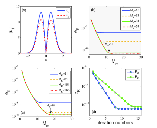
Figure 1: The amplitude distributions of the solitons for the two responses (a). $e_{R}$ versus $M_{m}$ for different $M_{k}$ respectively for $R_{G}(x)$ (b) and $R_{E}(x)$ (c). The $e_{R}$ diagrams versus the iteration numbers (d).

In the following, we are going to search a $\psi_{n}(x)$ under the expected degree of the nonlocality $\sigma=w_{mat}/w_{s}$, with $w_{mat}$ the characteristic length of the media and $w_{s}$ the root-mean-square(RMS) width of the soliton (expressed as $w_{s}=\sqrt{\int_{-\infty}^{+\infty}2x^{2}|\psi_{n}(x)|^{2}dx/\int_{-\infty}^{+\infty}|\psi_{n}(x)|^{2}dx}$). Since $w_{s}$ is unknown, we can use the RMS width of its zeroth-order approximation [$\phi_{n}^{(0)}(x)$] instead, which is $w=\mu\sqrt{2n+1}$W.Greiner-book-01 , and then give an apriori value of $\sigma$ which reads

$$\sigma=\frac{w_{mat}}{\mu\sqrt{2n+1}}.$$ (9)

The reason is that $w_{s}$ mainly depend on $\phi_{n}^{(0)}$ according to the expansion (7), and the higher-order corrections in the expansion only slightly deviate the RMS width $w_{s}$ from $w$, as will be discussed below. Therefore, by setting $\mu=w_{mat}/(\sigma\sqrt{2n+1})$, we determine a “minimum” $f_{n}(x)$ by means of the WLS methodWilliam H. Press-book-92 , of which the procedure is as follows. For a given transverse distribution of the optical beam $\sqrt{A_{n}}\psi_{n}(x)$, the deviation, which is sampled by the optical beam, between the nonlinear refraction and the parabolic refraction is

$$\delta(A_{n},V_{n0})=\int_{-\infty}^{\infty}f_{n}^{2}(x)\psi_{n}^{2}(x)dx.$$ (10)

By letting the first derivative of $\delta(A_{n},V_{n0})$ with respect to $A_{n}$ and that to $V_{n0}$ equal zero respectively, we have

$$\begin{cases}aA_{n}-bV_{n0}=d\\ bA_{n}-cV_{n0}=e,\end{cases}$$ (11)

where $a=\int_{-\infty}^{\infty}V^{2}_{n}(x)\psi_{n}^{2}(x)dx$, $b=\int_{-\infty}^{\infty}V_{n}(x)\psi_{n}^{2}(x)dx$, $c=\int_{-\infty}^{\infty}\psi_{n}^{2}(x)dx$, $d=\int_{-\infty}^{\infty}x^{2}V_{n}(x)\psi_{n}^{2}(x)dx/(2\mu^{4})$, $e=\int_{-\infty}^{\infty}x^{2}\psi_{n}^{2}(x)dx/(2\mu^{4})$, and $V_{n}(x)=-\int_{-\infty}^{\infty}R(x-\xi)\psi_{n}^{2}(\xi)d\xi$. By easily solving this equation set, $A_{n}$ and $V_{n0}$ can be obtained as

$$A_{n}=\frac{dc-be}{ac-b^{2}},~{}~{}V_{n0}=\frac{bd-ae}{ac-b^{2}}.$$ (12)

Then, the perturbation $f_{n}(x)$ which makes the deviation $\delta$ reaches its minimum is obtained through the relationships of Eq. (12). As a result, we can calculate $E_{n}$ and $\psi_{n}$ via Eqs. (6) and (7) by truncating the summations by the maxima of $m$ and $k$ (marked as $M_{m}$ and $M_{k}$, respectively) when the error of the numerical solution can hardly decreases.

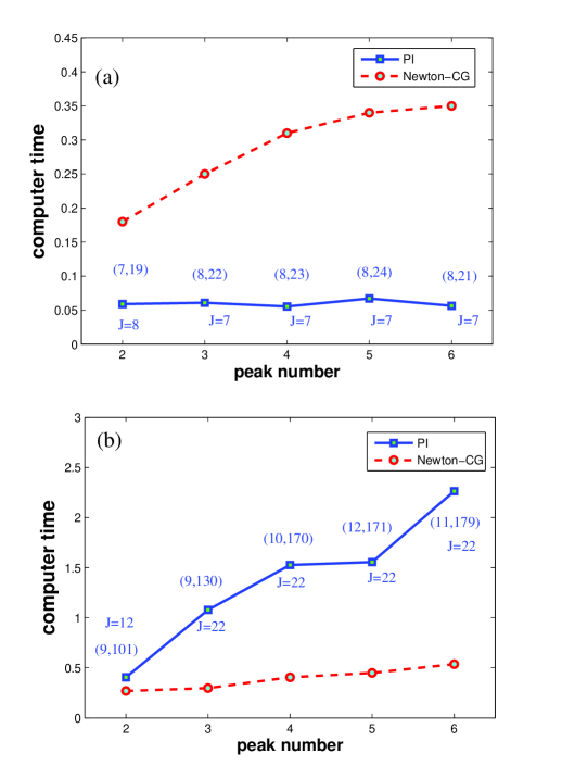
Figure 2: The comparisons of the computer times of the solitons with different $n$, taken by our method (PI) and the Newton-CG method, for $R_{G}(x)$ (a) and $R_{E}(x)$ (b), respectively. The needed values of the pair ($M_{m}$, $M_{k}$) and the iteration number $J$ for every soliton are marked.

We can repeat the above procedure to achieve higher accuracy by the iteration. First, we let $\psi_{n}^{(1)}=\phi_{n}^{(0)}$ as an input wave function [$\psi_{n}^{(j)}$ is the real wavefunction in the $j$-$th$ loop$(j=1,2,3...)]$, and algorithmize this procedure according to Eqs. (6), (7), and (12) through the following iterating process: within the $j$-$th$ loop, we have

$$A_{n}^{(j)}=\frac{d^{(j)}c^{(j)}-b^{(j)}e^{(j)}}{a^{(j)}c^{(j)}-(b^{(j)})^{2}},$$ (13)

$$V_{n0}^{(j)}=\frac{b^{(j)}d^{(j)}-a^{(j)}e^{(j)}}{a^{(j)}c^{(j)}-(b^{(j)})^{2}},$$ (14)

$$f_{n}^{(j)}=A_{n}^{(j)}V_{n}^{(j)}-V_{n0}^{(j)}-x^{2}/(2\mu^{4}),$$ (15)

$$E_{n}^{(j+1)}=\varepsilon_{n}^{(0)}+\sum_{m=1}^{M_{m}}\int_{-\infty}^{+\infty}\phi_{n}^{(0)}f_{n}^{(j)}\phi_{n}^{(m-1)}dx,$$ (16)

$$\psi_{n}^{(j+1)}=\phi_{n}^{(0)}+\sum_{m=1}^{M_{m}}\sum_{k=0(k\neq n)}^{M_{k}}\zeta_{mk}^{(j)}\phi_{k}^{(0)}.$$ (17)

At last, the soliton solutions of Eq. (1) are obtained as $u_{n}(x,z)=\sqrt{A_{n}^{(J)}}\psi_{n}^{(J+1)}(x)\exp(-i\beta_{n}z)\$ with $\beta_{n}=E_{n}^{(J+1)}+V_{n0}^{(J)}$, where $J$ is the number of iteration. Note that $E_{n}^{j+1}$ inside the loop is used to compute the error within the loop. In principle, $M_{k}$ for every $m$-order of the expansion(17) can be individually chosen. For the practical convenience, however, $M_{k}$ is set to the same value for every $m$-order in our computation below. .

For the obtained soliton solution with the form given by Eq. (2), the corresponding residual is

$$e_{A} =\left|\frac{\sqrt{A_{n}}}{2}\frac{d^{2}}{dx^{2}}\psi_{n}(x)-A_{n}^{3/2}\psi_{n}(x)V_{n}(x)+\sqrt{A_{n}}\beta_{n}\psi_{n}(x)\right|$$ (18)

$$=\sqrt{A_{n}}e_{R},$$

with

$$e_{R}=\left|\frac{1}{2}\frac{d^{2}}{dx^{2}}\psi_{n}(x)-A_{n}\psi_{n}(x)V_{n}(x)+\beta_{n}\psi_{n}(x)\right|.$$ (19)

Although the residual is the function of $x$, we consider its average value within the region quadruple larger than the width of the soliton, since the data in the domain far from the soliton are meaningless for discussing the error. Obviously, $e_{A}$ consists of $\sqrt{A_{n}}$ and $e_{R}$ that we defined as the relative residual, and $e_{R}$ is more reasonable than $e_{A}$ to be used to discuss the error of the numerical results, since $\sqrt{A_{n}}$ of the solitons with different $n$ are quite different. The iteration process are terminated when the criterion $\lambda\left(\lambda=\sqrt{\int_{-\infty}^{\infty}[\psi_{n}^{(j+1)}(x)-\psi_{n}^{(j)}(x)]^{2}dx}\right)$ is sufficiently small.

III Examples

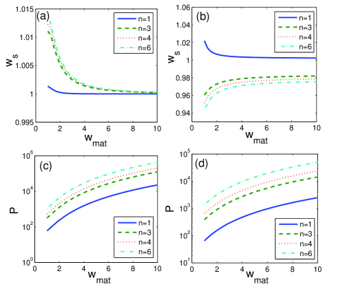
Figure 3: The widths of the solitons with different $n$ as the function of $w_{mat}$ for $R_{G}(x)$ (a) and $R_{E}(x)$ (b), respectively. The power of the solitons(shown in logarithmic coordinate) with different $n$ as the function of $w_{m}$ for $R_{G}(x)$ (c) and $R_{E}(x)$ (d), respectively.

.

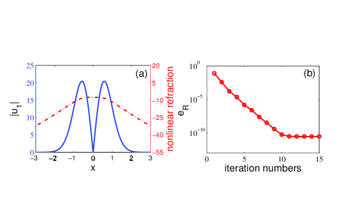
Figure 4: (a) The amplitude distribution of the 2-peak soliton (blue solid curve) and the distribution of its induced nonlinear refraction (red dashed curve) of the sine-oscillation response. (b) $e_{R}$ versus the number of iteration.

.

We show in Fig. 1 the computation of $2$-peak solitons ($n=1$) for Gaussian and exponential-decay response functions which respectively readsQi Guo-book-01 ; Qi Guo-book-02 $R_{G}(x)=\exp[-x^{2}/(2w_{mat}^{2})]/(\sqrt{2\pi}w_{mat})$ and $R_{E}(x)=\exp(-|x|/w_{mat})/(2w_{mat})$, where $w_{mat}$ is the characteristic length of the media. In our computation, for convenience, we let $\mu=1/\sqrt{2n+1}$ to make the RMS widths of $\phi_{n}^{(0)}$ equal to $1$, and then $\sigma=w_{mat}$ [see Eq. (9) above)], which is chosen to be $2$ in this example. The computational domain is taken as $-20<x<20$, discretized by 8192($2^{13}$) points (The below computations are the same with these parameters). Figure 1(a) are the amplitude distributions of the solitons for the two responses. In order to chose proper $M_{m}$ and $M_{k}$, we present the $e_{R}$ diagrams versus $M_{m}$ for different $M_{k}$ in Figs. 1(b) and (c) respectively for $R_{G}(x)$ and $R_{E}(x)$. Here we terminate the iterations when $\lambda$ is sufficiently small. For both two cases, it is clear that $e_{R}$ rapidly declines when $M_{m}$ increases and becomes nearly unchangeable. As $M_{k}$ keeps on increasing, $e_{R}$ also declines and becomes unchangeable. The results above indicate the best accuracy can be achieved when $M_{m}$ and $M_{k}$ are both large enough. In detail, for the $2$-peak solitons, $M_{m}=12$ and $M_{k}=31$ are found for $R_{G}(x)$ to reach the best accuracy of $2.1\times 10^{-11}$ and $M_{m}=18$ and $M_{k}=151$ for $R_{E}(x)$ to reach $1.5\times 10^{-10}$. However, for other achievable accuracies one required, it is difficult to obtain the proper values of $M_{m}$ and $M_{k}$ in a fast way. One can start for small values of $M_{m}$ and $M_{k}$ (typically, $M_{m}=3$ and $M_{k}=15$), fix the value of $M_{m}$ and increase $M_{k}$, until $e_{R}$ reaches the required value; if $e_{R}$ cannot reach the required value, then increase $M_{m}$ and repeat the procedure above. By setting $M_{m}$ and $M_{k}$ for the best accuracy mentioned above, we further calculate the $e_{R}$ diagrams versus the number of iterations shown in Fig. 1(d) for the cases of the two responses. It is shown that the $e_{R}$ rapidly declines with the iteration, and becomes nearly unchangeable when the number of the iteration is larger than $9$ and $13$ respectively for the cases of $R_{G}(x)$ and $R_{E}(x)$.

Our method can be used to calculate multi-peak solitons with an arbitrary order of soliton $n$. For the given $e_{R}=10^{-9}$, the computer times for the solitons with different $n$ are shown in Figs. 2(a) and (b) for $R_{G}(x)$ and $R_{E}(x)$, respectively. In addition, the needed values of the pair ($M_{m}$, $M_{k}$) and the iteration number $J$ for every soliton are marked in the figures. For comparison, the results taken by Newton-CG methodJ. Yang-jcp-09 are also presented. It is shown that our method takes even shorter times than the Newton-CG method for $R_{G}(x)$, but much longer times for $R_{E}(x)$, since the case of $R_{E}(x)$ takes much larger values of $M_{m}$, $M_{k}$ and $J$ than that of $R_{G}(x)$. Even so, our method is quite accessible, since the cost computer times are in the order of seconds, and the initial condition is fixed to $\phi_{n}^{(0)}(x)$, rather than careful choosing of an initial profile. Note that the Newton-CG method requires that the initial condition is reasonably close to the exact solutionJ. Yang-jcp-09 . In our realization of the Newton-CG method, therefore, we choose $B\phi_{n}^{(0)}(x)$ (with $B$ the initial amplitude) as the initial condition, and $B$ should be carefully chose to ensure the convergence of the iteration. Moreover, the sensitivity of $B$ also increases as the peak number increases, according to our computation.

We also present the RMS widths of the solitons $w_{s}$ with different $n$ as a function of the characteristic length $w_{mat}$, i.e, the degree of the nonlocality, for $R_{G}(x)$ and $R_{E}(x)$, which are shown in Figs. 3(a) and (b), respectively. The request values of $e_{R}$ are the same with those in Fig. 2. As expected above, the higher-order corrections in the expansion (7) only slightly deviate the RMS widths from $1$. As $w_{mat}$ increases, $w_{s}$ for the case of $R_{G}(x)$ tends to $1$, while that for the case of $R_{E}(x)$ tends to a value deviated from $1$. This asymptotic behavior can be understood as followsQi Guo-book-01 ; Qi Guo-book-02 : as $w_{mat}$ increases, namely, the degree of the nonlocality increases, Eq. (3) with $R_{G}(x)$ tends to the SM model, i.e., the model for harmonic oscillator described by Eq. (5) A. W. Snyder-Science-97 , and then $w_{s}$ tends to $1$; for the case of $R_{E}(x)$, in the strongly nonlocal limit, i.e., $w_{mat}\rightarrow\infty$, Eq. (3) does not tend to Eq. (5) due to the discontinuity in the derivative of $R_{E}(x)$ at the origin (detailed discussions can be found in Qi Guo-book-01 ; Qi Guo-book-02 ), therefore this deviation is in expectation. It is worth mentioning that the best of achievable $e_{R}$ is not sensitive to $w_{mat}$, i.e., the degree of the nonlocality, according to our computation. Figs. 3(c) and (d) are the power of the solitons (shown in logarithmic coordinate) with different $n$ as the function of $w_{mat}$ for $R_{G}(x)$ and $R_{E}(x)$, respectively. As $n$ and $w_{mat}$ increase, the power of the solitons increases rapidly, which is the reason why $e_{R}$ is more proper than $e_{A}$ to discuss the error of the solitons, as mentioned above.

Finally, we show in Fig. 4 the computation of the 2-peak soliton with the sine-oscillation response $R_{S}(x)=-\sin(|x|/w_{m})/(2w_{m})$sine1 ; sine2 , which could hardly be obtained by other known methods as far as we have tried. The best accuracy of $3.2\times 10^{-11}$ is achieved when $M_{m}=25$ and $M_{k}=179$. The physical properties for such multi-peak solitons with $R_{S}(x)$ will be further discussed otherwhere.

IV Conclusion

In this work, we develop a method for the numerical computations of the Hermite-Gauss-like solitons with arbitrary peak numbers in nonlocal nonlinear media. We start from the perturbed model of the harmonic oscillator, determine the “minimum” perturbation by means of the WLS method, and use the formal expression of infinite-order perturbation expansions to numerically calculate the eigenfunctions and eigenvalues of the perturbed model. Finally we iterate the procedure above to achieve a sufficient high accuracy. This method takes a few tens of iteration loops, and the initial condition is fixed to the Hermite-Gaussian function. It is worth mentioning that our method is not restricted to the NNLSE, but might also be able to be extended to the Schrödinger equations in any type of potentials.

V Funding Information

National Natural Science Foundation of China (Grant No. 11474109).

References

- (1) A. W. Snyder , D. J. Mitchell, “Accessible solitons,” Science, 276, 1538-1541 (1997).
- (2) G. Assanto, Nematicons: Spatial Optical Solitons in Nematic Liquid Crystals (New Jersey: John Wiley & Sons, 2013).
- (3) Qi Guo, Daquan Lu, and Dongmei Deng, Nonlocal spatial optical solitons, Chapter 4, in Advances in Nonlinear Optics, edited by X. Chen, Qi Guo, W. She, H. Zeng, and G. Zhang, (De Gruyter, Berlin, Feb. 2015), p.p.227-305.
- (4) A.W. Snyder and Y. Kivshar, “Fright spatial solitons in non-Kerr media: stationary beams and dynamical evolution ,” J. Opt. Soc. Am. B 11, 3025-3031 (1997).
- (5) A.W. Snyder, “Guiding light into the millennium ,” IEEE J. Sel. Top. Quantum Electron. 6, 1408-1412 (2000).
- (6) C. Conti, M. Peccianti, G. Assanto, “ Route to nonlocality and observation of accessible solitons,” Phys. Rev. Lett. 91, 073901 (2003).
- (7) C. Conti, M. Peccianti, G. Assanto, “Observation of optical spatial solitons in highly nonlocal medium,” Phys. Rev. Lett. 92, 113902 (2004).
- (8) M. Peccianti, C. Conti, G. Assanto,“All-optical switching and logic gating with spatial solitons in liquid crystals ,” Appl. Phys. Lett. 81, 3335-3337 (2002).
- (9) M. Peccianti, K. A. Brzdakiewicz, and G. Assanto,“Nonlocal spatial soliton interactions in nematic liquid crystals, ” Opt. Lett. 27, 1460-1462 (2002).
- (10) M. Peccianti, C. Conti, G. Assanto,“Optical modulational instability in a nonlocal medium, ” Phys. Rev. E 68, 025602 (2003).
- (11) D. N. Christodoulides, T. H. Coskun, M. Mitchell, Z. G. Chen, M. Segev, “Theory of incoherent dark solitons,” Phys. Rev. Lett. 80, 2310-2313 (1998).
- (12) A. V. Mamaev, A. A. Zozulya, V. K. Mezentsev, D. Z. Anderson, and M. Saffman,“ Bound dipole solitary solutions in anisotropic nonlocal self-focusing media ,” Phys. Rev. A 56, 1110-1113 (1997).
- (13) X. Hutsebaut, C. Cambournac, M. Haelterman, A. Adamski, and K. Neyts,“Single-component higher-order mode solitons in liquid crystals,” Opt. Commun. 233, 211-217(2004).
- (14) A. I. Yakimenko, V. M. Lashkin, and O. O. Prikhodko, “Dynamics of two-dimensional coherent structures in nonlocal nonlinear media,” Phys. Rev. E 73, 066605 (2006).
- (15) D. W. McLaughlin, D. J. Muraki, M. J. Shelley, “Self-focussed optical structures in a nematic liquid crystal,” Physica D 97, 471-497 (1996).
- (16) D. Deng, X. Zhao, Q. Guo , S. Lan, “Hermite-Gaussian breathers and solitons in strongly nonlocal nonlinear media,” J. Opt. Soc. Am. B 24,2537-2544 (2007).
- (17) D. Buccoliero, A. S. Desyatnikov, W. Krolikowski, and Y. S. Kivshar, “Laguerre and Hermite soliton clusters in nonlocal nonlinear media,” Phys. Rev. Lett. 98, 053901 (2007).
- (18) C. Rotschild, M. Segev, Z. Y. Xu, Y. V. Kartashov, L. Torner, and O. Cohen, “Two-dimensional multipole solitons in nonlocal nonlinear media,” Opt. Lett. 31, 3312-3314 (2006).
- (19) Z. Xu, Y. V. Kartashov, and L. Torner, “Upper threshold for stability of multipole-mode solitons in nonlocal nonlinear media,” Opt. Lett. 30, 3171-3173 (2005).
- (20) Dongmei Deng, Qi Guo, and Wei Hu, “Hermite-Laguerre-Gaussian beams in strongly nonlocal nonlinear media,” J. Phys. B: At. Mol. Opt., 41, 225402 (2008).
- (21) Dongmei Deng, and Qi Guo, “Ince-Gaussian solitons in strongly nonlocal nonlinear media,” Opt. Lett., 32, 3206-3208 (2007).
- (22) Dongmei Deng, Qi Guo, and Wei Hu, “Comeplex-variable-function-Gaussian solitions,” Opt. Lett, 34, 43-45 (2009).
- (23) J. Yang,“Internal oscillations and instability characteristics of (2+1)-dimensional solitons in a saturable nonlinear medium,” Phys. Rev. E 66, 026601 (2002).
- (24) V.I. Petviashvili, “On the equation of a nonuniform soliton,” Plasma Phys. 2, 469-472 (1976).
- (25) M.J. Ablowitz, Z.H. Musslimani,“Spectral renormalization method for computing self-localized solutions to nonlinear systems,” Opt. Lett. 30, 2140-2142 (2005).
- (26) T.I. Lakoba, J. Yang,“A generalized Petviashvili iteration method for scalar and vector Hamiltonian equations with arbitrary form of nonlinearity,” J. Comput. Phys. 226, 1668-1692 (2007).
- (27) J.J. Garcia-Ripoll, V.M. Perez-Garcia, “Optimizing Schrodinger functionals using Sobolev gradients: Applications to quantum mechanics and nonlinear optics,” SIAM J. Sci. Comput. 23, 1315-1333 (2001).
- (28) J. Yang, T.I. Lakoba,“Accelerated imaginary-time evolution methods for the computation of solitary waves,” Stud. Appl. Math. 120, 265-292 (2008).
- (29) J.P. Boyd, Chebyshev and Fourier Spectral Methods (Dover Publications, second edition, 2001).
- (30) J.P. Boyd, “Deleted residuals, the QR-factored Newton iteration, and other methods for formally overdetermined determinate discretizations of nonlinear eigenproblems for solitary, cnoidal, and shock waves,” J. Comput. Phys. 179, 216-237(2002).
- (31) William H. Press, Brian P. Flannery, Saul A. Teukolsky, William T. Vetterling, Numerical Recipes in C: the Art OF Scientific Computing (Cambridge University Press,second edition,1992)
- (32) J. Yang, T. I. Lakoba, “Universally-convergent squared-operator iteration methods for solitary waves in general nonlinear wave equations,” Stud. Appl. Math. 118, 153-197 (2007).
- (33) Jianke Yang, “Newton-conjugate-gradient methods for solitary wave computations,” J. Comput. Phys. 228, 7007-7024 (2009).
- (34) D.E. Pelinovsky, Y.A. Stepanyants, “Convergence of Petviashvili’s iteration method for numerical approximation of stationary solutions of nonlinear wave equations,” SIAM J. Numer. Anal. 42, 1110-1127 (2004).
- (35) J. Yang, B.A. Malomed, D.J. Kaup, “Embedded Solitons in Second-Harmonic-Generating Systems,” Phys. Rev. Lett. 83, 1958 (1999).
- (36) Shigen Ouyang, Qi Guo, and Wei Hu, “Perturbative analysis of generally nonlocal spatial optical solitons,” Phys. Rev. E 74, 036622 (2006).
- (37) W.Greiner, Quantum Mechanics An Introduction (Springer-Verlag, 4th edition,Berlin,2001).
- (38) A. Messiah, Quantum Mechanics (John Wiley & Sons, Inc, New York,1965), Vol.2, p.688.
- (39) In the Newton-CG method, the residuals diverges for the sine oscillation response as far as we can try.
- (40) Qi Guo, Wei Hu, Dongme Deng, Daquan Lu, and Shigen Ouyang, Features of strongly nonlocal spatial solitons, Chapter 2, in Nematicons: Spatial Optical Solitons in Nematic Liquid Crystals, edited by Gaetano Assanto (John Wiley & Sons, New Jersey, 2013), p.p.37-69.
- (41) B. K. Esbensen, M. Bache, W. Krolikowski, and O. Bang, “Quadratic solitons for negative effective second-harmonic diffraction as nonlocal solitons with periodic nonlocal response function,” Phys. Rev. A 86, 023849 (2012).
- (42) J. Wang, Y. Li, Q. Guo, and W. Hu, “Stabilization of nonlocal solitons by boundary conditions,” Opt. Lett. 39, 405-408 (2014).