Principal component analysis of the nonlinear coupling of harmonic modes in heavy-ion collisions

Abstract

The principal component analysis of flow correlations in heavy-ion collisions is studied. The correlation matrix of harmonic flow is generalized to correlations involving several different flow vectors. The method can be applied to study the nonlinear coupling between different harmonic modes in a double differential way in transverse momentum or pseudorapidity. The procedure is illustrated with results from the hydrodynamic model applied to Pb+Pb collisions at $\sqrt{s}=2760$ GeV. Three examples of generalized correlations matrices in transverse momentum are constructed corresponding to the coupling of $v_{2}^{2}$ and $v_{4}$, of $v_{2}v_{3}$ and $v_{5}$, or of $v_{2}^{3}$, $v_{3}^{3}$, and $v_{6}$. The principal component decomposition is applied to the correlation matrices and the dominant modes are calculated.

I Introduction

The expansion of the matter formed in relativistic heavy-ion collisions generates a collective transverse flow. The flow velocity field reflects the gradients in the initial density profile of the fireball. The harmonic coefficients of the azimuthal asymmetry of the spectra of emitted particles can be measured and compared to model predictions Heinz:2013th ; Gale:2013da ; Ollitrault:2010tn . The most notable examples are the elliptic $v_{2}$ and triangular $v_{3}$ flow coefficients.

Higher flow harmonics $v_{n}$, $n>3$, are coming from two sources, the expansion of the initial asymmetries of the source and due to the nonlinear coupling of lower order modes Teaney:2012ke . Correlations between flow harmonics of different order have been the subject of numerous theoretical Bhalerao:2011yg ; Qiu:2012uy ; Jia:2012ma ; Jia:2012ju ; Teaney:2013dta ; Yan:2015jma ; Noronha-Hostler:2015dbi ; Gardim:2016nrr ; Qian:2016fpi ; Qian:2017ier ; Zhu:2016puf ; Giacalone:2016afq ; Floerchinger:2013tya ; Bravina:2013ora and experimental studies Aad:2014fla ; ALICE:2016kpq ; Acharya:2017zfg ; Adamczyk:2017byf ; Tuo:2017ucz . One of the motivations was to find additional constraints on the initial state in heavy-ion collisions. What is even more important, the sensitivity of the linear and nonlinear response to the viscosity of the medium may serve as a tool to estimate of the value of shear viscosity in the deconfined quark-gluon plasma.

The correlations of flow harmonics at different transverse momenta Gardim:2012im or pseudorapidities Bozek:2010vz could reveal interesting information on fluctuations in the initial state of the evolution. A useful method to analyze the correlation matrix of flow harmonics is the principal component analysis (PCA) Bhalerao:2014mua . The procedure separates the leading and subleading components in the correlation matrix. The leading component corresponds to the usual flow and the subleading component is a measure of the flow factorization breaking at two different bins in phase space Mazeliauskas:2015vea ; Mazeliauskas:2015efa ; Cirkovic:2016kxt ; Sirunyan:2017gyb .

The correlation matrix for different flow harmonics reflects the mode mixing. Harmonic modes at different bins in phase space are partially decorrelated due to factorization breaking. The two effects can be combined by constructing a more general correlation matrix between different flow harmonics calculated at two different bins in phase space. This full correlation matrix can be decomposed into its principal components. The procedure analyzes the mixing of different modes in a double differential way in momentum.

I show examples from a hydrodynamic model for the PCA of the correlation matrices corresponding to the coupling of $v_{2}^{2}$ with $v_{4}$ and $v_{2}v_{3}$ with $v_{5}$. A correlation matrix of yet higher dimension is studied in the example of the correlation between the flow harmonics $v_{2}^{3}$, $v_{3}^{2}$, and $v_{6}$. In semi-central collisions a strong mixing of different modes is found.

II Principal component analysis of harmonic flow coefficients

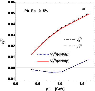
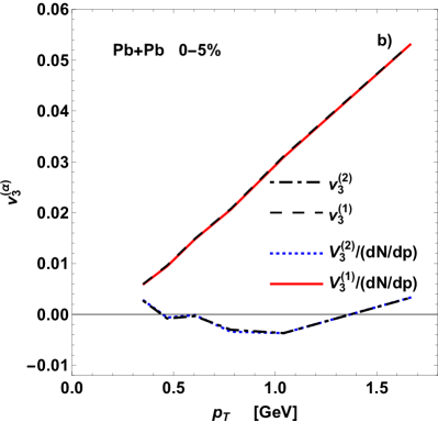
Figure 1: First (solid line) and second (dotted line) scaled eigenvectors $V_{n}^{(\alpha=1,2)}(p)/(dN/dp)$ of the correlation matrix $C_{n\Delta}(p_{1},p_{2})$ for the second (panel a) and third (panel b) order flow in Pb+Pb collisions at $\sqrt{s}=2760$ GeV and centrality $0-5$%. The dashed and dash-dotted lines represents the corresponding eigenvectors of the correlation matrix $c_{n\Delta}(p_{1},p_{2})$.

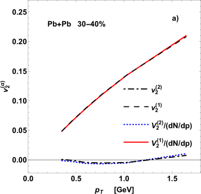
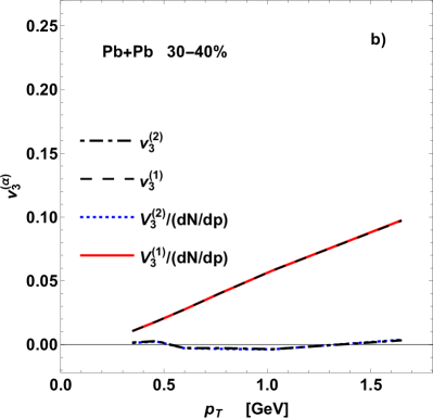
Figure 2: Same as in Fig. 1 but for Pb+Pb collisions with centrality $30-40$%.

The calculations are performed in a 3+1-dimensional viscous hydrodynamic model with event-by-event fluctuating initial conditions Schenke:2010rr ; Bozek:2011ua . The initial conditions are taken from a Glauber Monte Carlo model with quark degrees of freedom. The details of the calculation can be found in Bozek:2017elk . After the hydrodynamic expansion, particles are emitted statistically from the freeze-out hypersurface Chojnacki:2011hb .

For each hydrodynamic event many events are generated according to statistical emission from the freeze-out hypersurface. This allows to perform the calculation in two variants, the first using realistic events with nonflow correlations from resonance decays and the second using combined events from the same hydrodynamic evolution. The last method reduces fluctuations in observables involving several particles, which allows to estimate correlations with up to six flow vectors.

The correlation of flow harmonics Bhalerao:2014mua

$$C_{n\Delta}(p_{1},p_{2})=\langle Q_{n}(p_{1})Q_{n}^{\star}(p_{2})\rangle-\langle Q_{n}(p_{1})\rangle\langle Q_{n}^{\star}(p_{2})\rangle$$ (1)

is defined as the correlation of two flow vectors

$$Q_{n}(p)=\sum_{j}e^{in\phi_{j}}\ ,$$ (2)

where the sum is over all particles in the bin $p$, and $\langle\dots\rangle$ denotes the average over the events. The variable $p$ is the pseudorapidity or transverse momentum. The last term on the right hand side of Eq. 1 is needed only for multiplicity correlations, $n=0$. It is implicitly assumed that when the sums over the particles run over the same bin ($p_{1}=p_{2}$) self-correlation terms are subtracted. This gives an estimate of the correlation matrix of the collective flow at momenta $p_{1}$ and $p_{2}$.

Correlations of observables depending on transverse momentum are difficult to construct from the experimental data due to rapidly falling spectra. The correlations can be defined using transformed variables, with a flat spectrum Bialas:1990dk . The transformed variable $0<X<1$ is the cumulative probability for the distribution in transverse momentum $\frac{dN}{dp}$, $p_{min}<p<p_{max}$

$$X(p)=\frac{\int_{p_{min}}^{p}dp^{{}^{\prime}}\frac{dN}{dp^{{}^{\prime}}}}{\int_{p_{min}}^{p_{max}}dp^{{}^{\prime}}\frac{dN}{dp^{{}^{\prime}}}}\ .$$ (3)

By definition the distribution $\frac{dN}{dX}$ is flat. The correlation function $C_{n\Delta}(X_{1},X_{2})$ constructed in bins of the cumulative variable has uniform statistical uncertainties in all bins. This property makes the PCA more stable. Technically, the procedure is equivalent to using $k$ unequal bins in transverse momentum, corresponding to $k$ quantiles of the distribution $\frac{dN}{dp}$. Unless otherwise stated, I use 6 bins for $0.3$ GeV$<p<3$ GeV. For each bin the average $p$ is used to indicate the corresponding values on plots. In particular, the last bin is approximately $[1.2,3.0]$ GeV with the average value $1.66$ GeV for the centralities studied.

The eigenvalues $\lambda_{n}^{(\alpha)}$ and eigenvectors $\psi_{n}^{(\alpha)}(p)$ of the correlation matrix $C_{n\Delta}(p_{1},p_{2})$ are found

$$C_{n\Delta}(p_{1},p_{2}) = \sum_{\alpha}\lambda_{n}^{(\alpha)}\psi_{n}^{(\alpha)}(p_{1})\psi_{n}^{(\alpha)}(p_{2})$$ (4)

$$= \sum_{\alpha}V_{n}^{(\alpha)}(p_{1})V_{n}^{(\alpha)}(p_{2})\ .$$

Finally, eigenvectors are scaled by the multiplicity distribution $dN/dp$ as in Bhalerao:2014mua .

For correlations of flow coefficients $n>0$ the correlation of flow vectors normalized by the multiplicity

$$q_{n}=\frac{1}{n}\sum_{j}e^{in\phi_{j}}$$ (5)

can be constructed

$$c_{n\Delta}(p_{1},p_{2})=\langle q_{n}(p_{1})q_{n}^{\star}(p_{2})\rangle\ .$$ (6)

As before, for the same bin $(p_{1}=p_{2})$ self-correlations are avoided, and the normalization is by the number of pairs in the bins. The definition of the correlation matrix using the normalized $q_{n}$ vectors is useful for comparison to some models where the spectra and the collective flow is calculated without generating realistic finite multiplicity events. In the following the correlation matrices with upper case $C$ and lower case $c$ denote correlation of flow vectors $Q$ and $q$ respectively. The eigenvectors of correlation matrix $c$ are denoted with a lower case letter $v_{n}^{(\alpha)}(p)$

$$c_{n\Delta}(p_{1},p_{2})=\sum_{\alpha}v_{n}^{(\alpha)}(p_{1})v_{n}^{(\alpha)}(p_{2})\ .$$ (7)

Note that there is no need to scale the eigenvectors $v_{n}^{(\alpha)}(p)$ by the average multiplicity.

The scaled eigenvectors of the harmonic flow correlations of second and third order are shown in Figs. 1 and 2 for Pb+Pb collisions with centralities $0-5$% and $30-40$% respectively. The largest eigenvalue is dominant in the decomposition of the correlations matrix. It is consistent with the small factorization breaking of flow coefficient in transverse momentum Bhalerao:2014mua . On the same figures are plotted the eigenvectors of the correlation matrices $c_{n\Delta}(p_{1},p_{2})$ for the multiplicity normalized $q_{n}(p)$ vectors. The results are very similar to the eigenvectors of the correlations matrices $C_{n\Delta}(p_{1},p_{2})$.

III Principal component analysis of coupled flow harmonics

Harmonics of different order can be coupled due to correlations in the initial distribution of eccentricities or due to nonlinearities in the evolution Bhalerao:2011yg ; Yan:2015jma ; Noronha-Hostler:2015dbi ; Gardim:2016nrr ; Qian:2016fpi ; Qian:2017ier ; Zhu:2016puf ; Giacalone:2016afq . The mixed flow harmonics are usually calculated in a given acceptance region. More generally any mixed flow harmonic can be estimated using different bins in momentum. The simplest class of such correlators Bhalerao:2011yg defined for two bins in momentum is

$$v\{n_{1}\dots n_{l},-m_{1}\dots-m_{k}\}(p_{1},p_{2}) = \langle Q_{n_{1}}(p_{1})\dots Q_{n_{l}}(p_{1})Q_{m_{1}}^{\star}(p_{2})\dots Q_{m_{k}}^{\star}(p_{2})\rangle$$ (8)

$$= \langle\sum_{j_{1}\neq\dots\neq j_{l}}\sum_{s_{1}\neq\dots\neq s_{k}}e^{i(n_{1}\phi_{j_{1}}+\dots+n_{l}\phi_{j_{l}}-m_{1}\phi_{s_{1}}-\dots-m_{k}\phi_{s_{k}})}\rangle$$

the first and second sums run over particles in bins $p_{1}$ and $p_{2}$ respectively and $N=\sum_{i=1}^{l}n_{i}=\sum_{j=1}^{k}m_{k}$ . The above formula defines a (in general asymmetric) correlation matrix in momenta. Mode mixing suggests to study correlations of different possible harmonic of order $N$ in the bin $p_{1}$ and of order $N$ in the bin $p_{2}$. The full correlation matrix of order involves all such possible combinations of flow harmonics

$$C_{n\dots|m\dots|q\dots|\dots}(p_{1}^{I},p_{1}^{II},p_{1}^{III},\dots|p_{1}^{I},p_{1}^{II},p_{1}^{III},\dots) =$$

$$\begin{bmatrix}v\{n\dots,-n\dots\}(p_{1}^{I},p_{2}^{I})&v\{n\dots,-m\dots\}(p_{1}^{I},p_{2}^{II})&v\{n\dots,-q\dots\}(p_{1}^{I},p_{2}^{III})&\dots\\ v\{m\dots,-n\dots\}(p_{1}^{II},p_{2}^{I})&v\{m\dots,-m\dots\}(p_{1}^{II},p_{2}^{II})&v\{m\dots,-q\dots\}(p_{1}^{II},p_{2}^{III})&\dots\\ v\{q\dots,-n\dots\}(p_{1}^{III},p_{2}^{I})&v\{q\dots,-m\dots\}(p_{1}^{IIII},p_{2}^{II})&v\{q\dots,-q\dots\}(p_{1}^{IIII},p_{2}^{III})&\dots\\ \dots&\dots&\dots&\dots\end{bmatrix}\ .$$ (9)

The matrix $C_{n\dots|m\dots|q\dots|\dots}(p_{1}^{I},p_{1}^{II},p_{1}^{III},\dots|p_{1}^{I},p_{1}^{II},p_{1}^{III},\dots)$ is symmetric. Note that the dimension of the correlation matrix is the multiple of the dimension of the simple $C_{n\Delta}$ correlation matrices; it is indicated by the multiple momentum indices for the rows and columns of the matrix. For flow dominated correlations $C_{n\dots|m\dots|q\dots|\dots}(p_{1}^{I},p_{1}^{II},p_{1}^{III},\dots|p_{1}^{I},p_{1}^{II},p_{1}^{III},\dots)$ is positive semi-definite.

The most interesting correlations involve harmonic modes with strong coupling. In particular, from the most general form of the correlation matrix of order $N$ a submatrix can be chosen for which the off-diagonal terms in Eq. 9 are significant. In the following are listed few examples of such correlation matrices.

The coupling of $v_{2}^{2}$ harmonic to $v_{4}$ is defined by the matrix

$$C_{2;2|4}(p_{1}^{I},p_{1}^{II}|p_{2}^{I},p_{2}^{II})=\begin{bmatrix}\langle Q_{2}(p_{1}^{I})^{2}Q_{2}^{\star}(p_{2}^{I})^{2}\rangle&\langle Q_{2}(p_{1}^{I})^{2}Q_{4}^{\star}(p_{2}^{II})\rangle\\ \langle Q_{4}(p_{1}^{II})Q_{2}^{\star}(p_{2}^{I})^{2}\rangle&\langle Q_{4}(p_{1}^{II})Q_{4}^{\star}(p_{2}^{II})\rangle\end{bmatrix}$$ (10)

As discussed in section II the analogous correlation for normalized $q$ vector is

$$c_{2;2|4}(p_{1}^{I},p_{1}^{II}|p_{2}^{I},p_{2}^{II})=\begin{bmatrix}\langle q_{2}(p_{1}^{I})^{2}q_{2}^{\star}(p_{2}^{I})^{2}\rangle&\langle q_{2}(p_{1}^{I})^{2}q_{4}^{\star}(p_{2}^{II})\rangle\\ \langle q_{4}(p_{1}^{II})q_{2}^{\star}(p_{2}^{I})^{2}\rangle&\langle q_{4}(p_{1}^{II})q_{4}^{\star}(p_{2}^{II})\rangle\end{bmatrix}\ .$$ (11)

The nonlinear coupling of $v_{2}v_{3}$ and $v_{5}$ shows up in the correlation matrix

$$c_{23|5}(p_{1}^{I},p_{1}^{II}|p_{2}^{I},p_{2}^{II})=\begin{bmatrix}\langle q_{2}(p_{1}^{I})q_{3}(p_{1}^{I})q_{2}^{\star}(p_{2}^{I})q_{3}^{\star}(p_{2}^{I})\rangle&\langle q_{2}(p_{1}^{I})q_{3}(p_{1}^{I})q_{5}^{\star}(p_{2}^{II})\rangle\\ \langle q_{5}(p_{1}^{II})q_{2}^{\star}(p_{2}^{I})q_{3}^{\star}(p_{2}^{I})\rangle&\langle q_{5}(p_{1}^{II})q_{5}^{\star}(p_{2}^{II})\rangle\end{bmatrix}\ .$$ (12)

A more complicated matrix with coupling in three sectors $v_{2}^{3}$, $v_{3}^{2}$, and $v_{6}$ is

$$c_{2;3|3;2|6}(p_{1}^{I},p_{1}^{II},p_{1}^{III}|p_{2}^{I},p_{2}^{II},p_{2}^{III})=\begin{bmatrix}\langle q_{2}(p_{1}^{I})^{3}q_{2}^{\star}(p_{2}^{I})^{3}\rangle&\langle q_{2}(p_{1}^{I})^{3}q_{3}^{\star}(p_{2}^{II})^{2}\rangle&\langle q_{2}(p_{1}^{I})^{3}q_{6}^{\star}(p_{2}^{III})\rangle\\ \langle q_{3}(p_{1}^{II})^{2}q_{2}^{\star}(p_{2}^{I})^{3}\rangle&\langle q_{3}(p_{1}^{II})^{2}q_{3}^{\star}(p_{2}^{II})^{2}\rangle&\langle q_{3}(p_{1}^{II})^{2}q_{6}^{\star}(p_{2}^{III})\rangle\\ \langle q_{6}(p_{1}^{III})q_{2}^{\star}(p_{2}^{I})^{3}\rangle&\langle q_{6}(p_{1}^{III})q_{3}^{\star}(p_{2}^{II})^{2}\rangle&\langle q_{6}(p_{1}^{III})q_{6}^{\star}(p_{2}^{III})\rangle\end{bmatrix}\ .$$ (13)

Any submatrix of a more general matrix operators correlations can be considered

$$c_{2;3|6}(p_{1}^{I},p_{1}^{II}|p_{2}^{I},p_{2}^{II})=\begin{bmatrix}\langle q_{2}(p_{1}^{I})^{3}q_{2}^{\star}(p_{2}^{I})^{3}\rangle&\langle q_{2}(p_{1}^{I})^{3}q_{6}^{\star}(p_{2}^{II})\rangle\\ \langle q_{6}(p_{1}^{II})q_{2}^{\star}(p_{2}^{I})^{3}\rangle&\langle q_{6}(p_{1}^{II})q_{6}^{\star}(p_{2}^{II})\rangle\end{bmatrix}$$ (14)

or

$$c_{3;2|6}(p_{1}^{I},p_{1}^{II}|p_{2}^{I},p_{2}^{II})=\begin{bmatrix}\langle q_{3}(p_{1}^{I})^{2}q_{3}^{\star}(p_{2}^{I})^{2}\rangle&\langle q_{3}(p_{1}^{I})^{2}q_{6}^{\star}(p_{2}^{II})\rangle\\ \langle q_{6}(p_{1}^{II})q_{3}^{\star}(p_{2}^{I})^{2}\rangle&\langle q_{6}(p_{1}^{II})q_{6}^{\star}(p_{2}^{II})\rangle\end{bmatrix}\ .$$ (15)

The correlation matrices can be decomposed in eigenvectors in the same way as the correlation $c_{n\Delta}(p_{1},p_{2})$

$$c_{\dots}(p_{1}^{I},p_{1}^{I},\dots|p_{2}^{I},p_{2}^{II},\dots) = \sum_{\alpha}\lambda_{\dots}^{(\alpha)}\psi_{\dots}^{(\alpha})(p_{1}^{I},p_{1}^{II},\dots)\psi_{\dots}^{(\alpha)}(p_{2}^{I},p_{2}^{II},\dots)$$ (16)

$$= \sum_{\alpha}v_{\dots}^{(\alpha)}(p_{1}^{I},p_{1}^{II},\dots)v_{\dots}^{(\alpha)}(p_{2}^{I},p_{2}^{II},\dots)\ ,$$

with $v_{\dots}^{\alpha}(p_{1}^{I},p_{1}^{II},\dots)=\sqrt{\lambda_{\dots}^{\alpha}}\psi_{\dots}^{\alpha}(p_{1}^{I},p_{1}^{II},\dots)$. Note that the eigenvectors have a higher dimension than for the correlations $c_{n\Delta}(p_{1},p_{2})$, e.g.

$$v^{(\alpha)}_{2;2|4}(p^{I},p^{II})=\begin{bmatrix}v^{(\alpha,I)}_{2;2|4}(p^{I})\\ v^{(\alpha,II)}_{2;2|4}(p^{II})\end{bmatrix}$$ (17)

or

$$v^{(\alpha)}_{2;3|3;2|6}(p^{I},p^{II},p^{III})=\begin{bmatrix}v^{(\alpha,I)}_{2;3|3;2||6}(p^{I})\\ v^{(\alpha,II)}_{2;3|3;2||6}(p^{II})\\ v^{(\alpha,III)}_{2;3|3;2||6}(p^{III})\end{bmatrix}\ .$$ (18)

In the limit, when the mixing of different harmonic components in $c_{\dots}$ is negligible the dominant components of the first eigenvectors $v_{\dots}^{(q)}$ are close to the moments the relevant harmonic operators. For example the eigenvectors of $c_{2;2|4}$ would be

$$v_{2;2|4}^{(\alpha)}(p^{I},p^{II})\simeq\begin{bmatrix}0\\ \sqrt{\langle v_{4}(p^{II})^{2}\rangle}\end{bmatrix}$$ (19)

or

$$v_{2;2|4}^{(\alpha)}(p^{I},p^{II})\simeq\begin{bmatrix}\sqrt{\langle v_{2}(p^{I})^{4}\rangle}\\ 0\end{bmatrix}\ ,$$ (20)

for $\alpha=1,2$.

IV Hydrodynamic model results

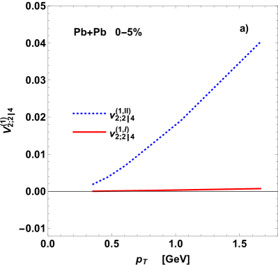
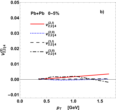
Figure 3: Eigenvectors of the correlation matrix $c_{2;2|4}$ (Eq. 11). Panel a), the two components of the first eigenvector; panel b), the two components of the second and third eigenvectors; Pb+Pb collisions with centrality $0-5$%.

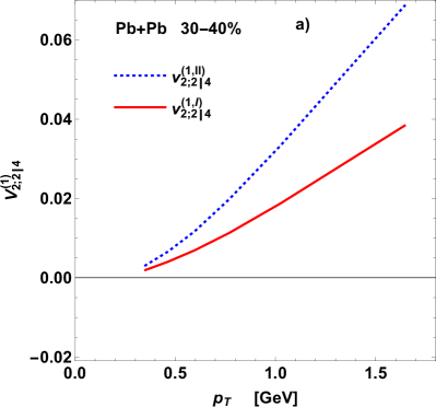
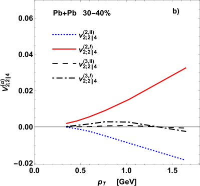
Figure 4: Same as in Fig. 3 but for collisions with centrality $30-40$%.

The hydrodynamic results presented in this section serve as an illustration of the possibility to perform the PCA for the generalized correlation matrices. Extensive, high statistics simulations for different initial conditions and viscosities are beyond the scope of this paper. The correlations in this section are calculated combining many events in same the hydrodynamic evolution. Thus, statistical fluctuations and nonflow effects are reduced.

The nonlinear coupling between $v_{2}^{2}$ and $v_{4}$ is expected to be significant whenever the elliptic flow is strong. The results of the decomposition in principal components for the correlator $c_{2;2|4}$ (Eq. 11) are shown in Figs. 3 and 4. For central collisions $0-5$% the nonlinear effects are small. The leading mode is located in the sector $v_{6}$ (Fig. 3 panel a)). The subleading mode is located in the sector $v_{2}^{2}$ with small mixing to $v_{6}$ (Fig. 3 panel b)). Only in the third mode a momentum dependent factorization breaking effect shows up clearly in the sector $v_{6}$.

The mixing of the modes $v_{2}^{2}$ and $v_{4}$ is stronger for semi-central collisions $30-40$%. The leading and the subleading modes have significant components in both sectors (Fig. 4). This mixing can be understood as due to a nonlinear contribution to the $v_{4}$ flow Teaney:2012ke

$$v_{4}=v_{4}^{L}+\chi_{422}v_{2}^{2}\ .$$ (21)

The PCA of the correlation matrix $c_{22;2|4}$ in momentum takes into account this nonlinear coupling, while being sensitive to possible additional effects of factorization breaking $\langle v_{2}(p_{1})v_{2}(p_{2})\rangle\neq\sqrt{\langle v_{2}(p_{1})^{2}\rangle\langle v_{2}(p_{2})^{2}\rangle}$ and of a momentum dependence of the coupling $\chi_{422}$. The third mode $v_{2;2|4}^{(3)}$ shows a momentum dependent factorization breaking, mainly in the sector $v_{4}$.

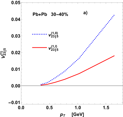
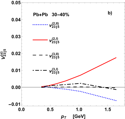
Figure 5: Same as in Fig. 4 for the correlation matrix $c_{23|5}$.

The flow $v_{5}$ get a contribution trough nonlinear coupling from the harmonic flow $v_{2}v_{3}$. In Fig. 5 are shown the first three eigenvectors for the correlation matrix $c_{23|5}$ (Eq. 12). The results are qualitatively similar to the case of $v_{2}^{2}$-$v_{4}$ coupling. The mixing between the modes $v_{2}v_{3}$ and $v_{5}$ is strong for the first two eigenvectors. The third eigenvector reflects the factorization breaking in momentum.

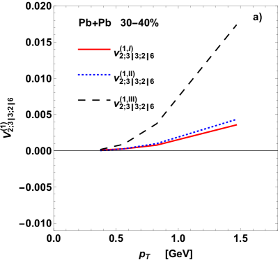
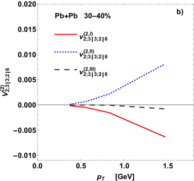
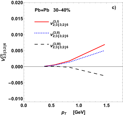
Figure 6: Eigenvectors of the correlation matrix $c_{2;3|3;2|6}$. In panels a) through d) are shown the components of the eigenvectors corresponding to the first four eigenvalues. In all panels three components of the eigenvectors are shown I (solid lines), II (dotted lines), and III (dashed lines) corresponding to the sectors $q_{2}(p)^{2}$, $q_{3}(p)^{3}$, and $q_{6}(p)$ in the correlation matrix.

The correlation matrix $c_{2;3|3;2|6}$ combines the flow vectors from three sectors $v_{2}^{3}$, $v_{3}^{2}$, and $v_{6}$. This correlation is calculated using 4 bins in transverse momentum only. As before the unequal bins correspond to 4 quantiles of the distribution $dN/dp$ in the range $[0.3,\ 3]$ GeV. The correlation matrix $c_{2;3|3:2|6}$ has dimensions $12\times 12$, with three sectors $v_{2}^{3}$, $v_{3}^{2}$, and $v_{6}$.

The first four eigenvectors are plotted in panels a) through d) in Fig. 6. The leading mode is a mixing in all three sectors with the strongest component from $v_{6}$. The second and third modes show a strong mixing in the $v_{2}^{3}$ and $v_{3}^{2}$ sectors with almost equal strength. The fourth mode shows a momentum dependent response Mazeliauskas:2015vea ; Mazeliauskas:2015efa , mainly in the $v_{6}$ sector.

The coupling between different harmonic modes is usually studied for the momentum integrated flow Giacalone:2016afq ; Yan:2015jma ; Qian:2016fpi ; Zhu:2016puf , with the exception of Ref. Qian:2017ier . In the present formalism, it corresponds to correlation matrices constructed with only one bin in transverse momentum. For the examples studied one has $2\times 2$ or $3\times 3$ matrices

$$c_{2;2|4}=\begin{bmatrix}\langle q_{2}^{2}q_{2}^{\star 2}\rangle&\langle q_{2}^{2}q_{4}^{\star}\rangle\\ \langle q_{4}q_{2}^{\star 2}\rangle&\langle q_{4}q_{4}^{\star}\rangle\end{bmatrix}\ ,$$ (22)

$$c_{23|5}=\begin{bmatrix}\langle q_{2}q_{3}q_{2}^{\star}q_{3}^{\star}\rangle&\langle q_{2}q_{3}q_{5}^{\star}\rangle\\ \langle q_{5}q_{2}^{\star}q_{3}^{\star}\rangle&\langle q_{5}q_{5}^{\star}\rangle\end{bmatrix}\ ,$$ (23)

and

$$c_{2;3|3;2|6}=\begin{bmatrix}\langle q_{2}^{3}q_{2}^{\star 3}\rangle&\langle q_{2}^{3}q_{3}^{\star 2}\rangle&\langle q_{2}^{3}q_{6}^{\star}\rangle\\ \langle q_{3}^{2}q_{2}^{\star 3}\rangle&\langle q_{3}^{2}q_{3}^{\star 2}\rangle&\langle q_{3}^{2}q_{6}^{\star}\rangle\\ \langle q_{6}q_{2}^{\star 3}\rangle&\langle q_{6}q_{3}^{\star 2}\rangle&\langle q_{6}q_{6}^{\star}\rangle\\ \end{bmatrix}\ .$$ (24)

The components of the two eigenvectors of the matrices $c_{2;2|4}$, $c_{23|5}$ agree qualitatively with the hierarchy of the components of the first two eigenvectors of the momentum dependent correlation matrices shown in Figs. 3, 4, and 5. Analogously, the hierarchy of the component of the three eigenvectors of $c_{2;3|3;2|6}$ (Eq. 24) reflects qualitatively the hierarchy of the components I, II, and III of the eigenvectors $v_{2;3|3;2|6}^{(\alpha)}$ in Fig. 6 for $\alpha=1,2,3$.

V Conclusions

The flow pattern in heavy-ion collisions reflects on event-by-event basis the fluctuations and correlations present in the initial state as well as the development of different modes in the hydrodynamic evolution. The study of flow harmonics and their correlations gives constraints both on the initial state and on the properties of the expanding dense matter in the fireball. I propose to study the correlations between different flow harmonics at two different transverse momenta (or pseudorapidities).

The full correlation matrix has a block structure. Each block can be either a correlation matrix between the same flow harmonics at two different momenta or a correlations of two different flow harmonics at two different momenta. The PCA is performed on this generalized correlation matrix. One finds momentum dependent eigenmodes corresponding to the modes resulting from the mixing of different harmonics. For a correlation matrix build out of $n$ different harmonics the first $n$ eigenvectors reflect mostly the mode mixing. Only higher eigenvectors show the weak component due to factorization breaking.

Model simulations and experimental measurements of the correlation matrix between different flow harmonics yield additional information on harmonic mode mixing in heavy-ion collisions. The PCA performed in transverse momentum is a method to study mode mixing at different momenta and factorization breaking in the same framework. A double differential study in transverse momentum or rapidity could also identify sources of mode mixing other than collective flow.

- (1) U. Heinz and R. Snellings, Ann.Rev.Nucl.Part.Sci. 63, 123 (2013)
- (2) C. Gale, S. Jeon, and B. Schenke, Int.J.Mod.Phys. A28, 1340011 (2013)
- (3) J.-Y. Ollitrault, J. Phys. Conf. Ser. 312, 012002 (2011)
- (4) D. Teaney and L. Yan, Phys. Rev. C86, 044908 (2012)
- (5) R. S. Bhalerao, M. Luzum, and J.-Y. Ollitrault, Phys. Rev. C84, 034910 (2011)
- (6) Z. Qiu and U. Heinz, Phys. Lett. B717, 261 (2014)
- (7) J. Jia and S. Mohapatra, Eur. Phys. J. C73, 2510 (2013)
- (8) J. Jia and D. Teaney, Eur. Phys. J. C73, 2558 (2013)
- (9) D. Teaney and L. Yan, Phys. Rev. C90, 024902 (2014)
- (10) L. Yan and J.-Y. Ollitrault, Phys. Lett. B744, 82 (2015)
- (11) J. Noronha-Hostler, L. Yan, F. G. Gardim, and J.-Y. Ollitrault, Phys. Rev. C93, 014909 (2016)
- (12) F. G. Gardim, F. Grassi, M. Luzum, and J. Noronha-Hostler, Phys. Rev. C95, 034901 (2017)
- (13) J. Qian, U. W. Heinz, and J. Liu, Phys. Rev. C93, 064901 (2016)
- (14) J. Qian, U. Heinz, R. He, and L. Huo, Phys. Rev. C95, 054908 (2017)
- (15) X. Zhu, Y. Zhou, H. Xu, and H. Song, Phys. Rev. C95, 044902 (2017)
- (16) G. Giacalone, L. Yan, J. Noronha-Hostler, and J.-Y. Ollitrault, Phys. Rev. C94, 014906 (2016)
- (17) S. Floerchinger, U. A. Wiedemann, A. Beraudo, L. Del Zanna, G. Inghirami, and V. Rolando, Phys. Lett. B735, 305 (2014)
- (18) L. V. Bravina, B. H. Brusheim Johansson, G. K. Eyyubova, V. L. Korotkikh, I. P. Lokhtin, L. V. Malinina, S. V. Petrushanko, A. M. Snigirev, and E. E. Zabrodin, Phys. Rev. C89, 024909 (2014)
- (19) G. Aad et al. (ATLAS Collaboration), Phys. Rev. C90, 024905 (2014)
- (20) J. Adam et al. (ALICE Collaboration), Phys. Rev. Lett. 117, 182301 (2016)
- (21) S. Acharya et al. (ALICE Collaboration), Phys. Lett. B773, 68 (2017)
- (22) L. Adamczyk et al. (STAR Collaboration)(2017), arXiv:1701.06497 [nucl-ex]
- (23) S. Tuo (CMS Collaboration), Nucl. Phys. A967, 381 (2017)
- (24) F. G. Gardim, F. Grassi, M. Luzum, and J.-Y. Ollitrault, Phys.Rev. C87, 031901 (2013)
- (25) P. Bożek, W. Broniowski, and J. Moreira, Phys. Rev. C83, 034911 (2011)
- (26) R. S. Bhalerao, J.-Y. Ollitrault, S. Pal, and D. Teaney, Phys. Rev. Lett. 114, 152301 (2015)
- (27) A. Mazeliauskas and D. Teaney, Phys. Rev. C91, 044902 (2015)
- (28) A. Mazeliauskas and D. Teaney, Phys. Rev. C93, 024913 (2016)
- (29) P. Cirkovic, D. Devetak, M. Dordevic, J. Milosevic, and M. Stojanovic, Chin. Phys. C41, 074001 (2017)
- (30) A. M. Sirunyan et al. (CMS)(2017), arXiv:1708.07113 [nucl-ex]
- (31) B. Schenke, S. Jeon, and C. Gale, Phys. Rev. Lett. 106, 042301 (2011)
- (32) P. Bożek, Phys. Rev. C85, 034901 (2012)
- (33) P. Bożek and W. Broniowski, Phys. Rev. C96, 014904 (2017)
- (34) M. Chojnacki, A. Kisiel, W. Florkowski, and W. Broniowski, Comput. Phys. Commun. 183, 746 (2012)
- (35) A. Bialas and M. Gazdzicki, Phys. Lett. B252, 483 (1990)