Polynomial Approximations of Hysteresis Curves Near the Demagnetized State

Abstract

Polynomial approximations of hysteresis curves were studied for systems exhibiting the return point memory. An extended Rayleigh law that uses polynomials of the third degree, and Rayleigh-like equations describing the energy dependence on the applied magnetic field are proposed. The results were compared with numerical experiments on a zero temperature random bond Ising model.

1 Introduction

Symmetric hysteresis loop and the virgin magnetization curve in the neighborhood of the demagnetized state are described by the equations

$$M=(a+bH_{m})H\pm\frac{b}{2}(H^{2}-H_{m}^{2}),\qquad M=aH\pm bH^{2},$$ (1)

where the upper and lower signs distinguish the ascending and descending branches. Equations (1) represent the so-called Rayleigh law [2, 3, 1, 5], named after Lord Rayleigh, who discovered them experimentally [13]. Rayleigh equations have been confirmed for many ferromagnetic materials. Neel gave the first explanation of the Rayleigh law in terms of domain walls moving in a random energy landscape [10, 11]. For recent development in the microscopic foundation of the Rayleigh law see, e.g., [16] and references therein.

This work does not concern details of the underlying mechanism responsible for the Rayleigh law. Instead, restrictions on hysteresis curves imposed by the return point memory, also called “wiping out” property, [1, 9, 14] are studied. The consideration is based on the results of the previous work [8] that are summarized below for convenience of the reader.

Let the slowly varying uniaxial magnetic field $H(t)$ is applied to a demagnetized ferromagnetic specimen. Let $H$ decreases by $\Delta H_{0}$ starting from the value $H=0$, then increases by $\Delta H_{1}$, then decreases by $\Delta H_{2}$ and so on till $\Delta H_{n}$, as shown in Fig. 1. The final macroscopic state of the specimen is completely determined by the sequence $\Delta H_{0},\ldots,\Delta H_{n}$, where $n$ can be any number, $n=0,1,\,\ldots$ .

If the specimen exhibits the return point memory (RPM), all the states that can be obtained by applying $H(t)$, can be reached by the process such that

$$2\Delta H_{0}>\Delta H_{1}>\ldots\Delta H_{n}>0.$$ (2)

These values are considered as coordinates in the so called “minimal space of states”, which includes all and only the states reachable from the demagnetized state by applying $H(t)$.

It is convenient to designate

$$\xi_{0}=2\Delta H_{0},\,\xi_{1}=\Delta H_{1},\,\xi_{2}=\Delta H_{2},\,\ldots,\,\xi_{n}=\Delta H_{n}$$ (3)

and assume that

$$\xi_{0}\geq\xi_{1}\geq\xi_{2}\geq\ldots\geq\xi_{n}\geq 0.$$ (4)

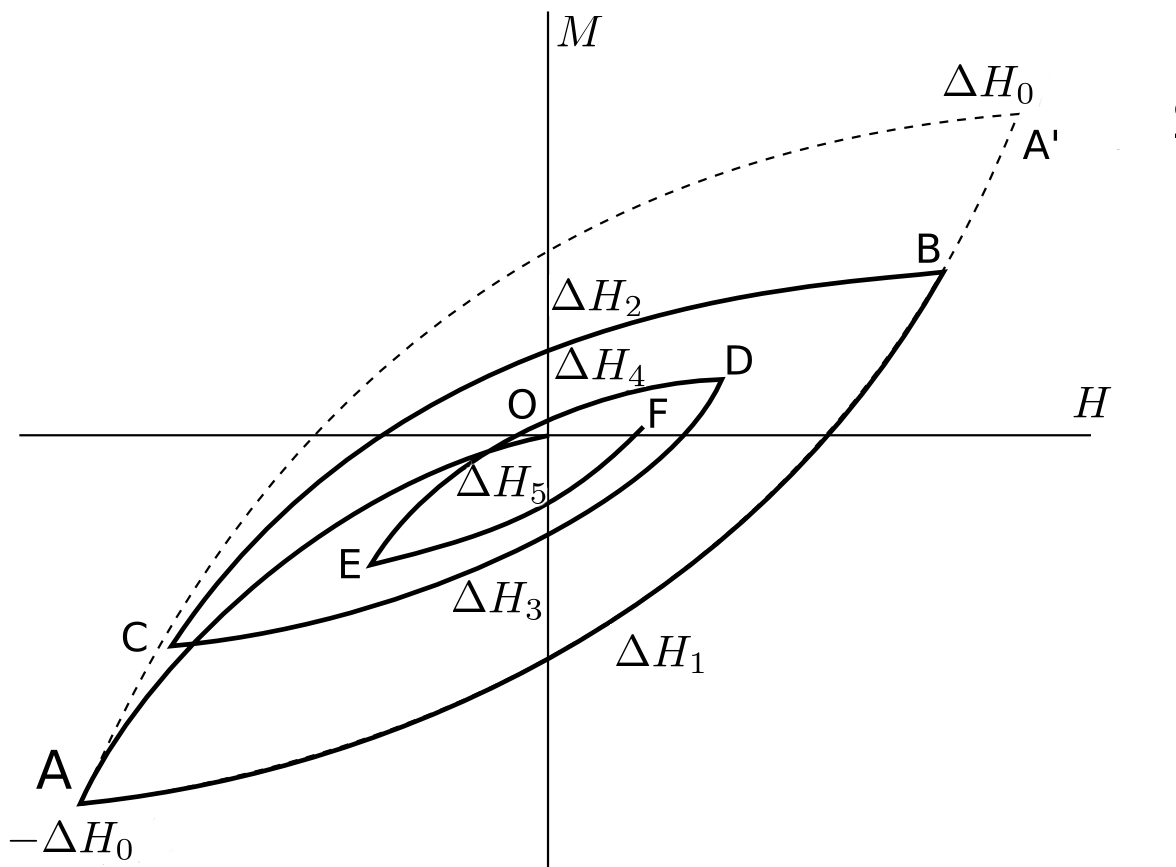
Figure 1: Magnetization process $OABCDEF$ starts from the demagnetized state at the point $O$ and is performed by decreasing the field $H$ by the value $\Delta H_{0}$, then increasing it by $\Delta H_{1}$, then decreasing it by $\Delta H_{2}$ and so on. The final state of the system is determined by the values $\Delta H_{0},\ldots,\Delta H_{n}$, where $n+1$ is the number of hysteresis branches. The symmetric cycle $AA^{\prime}$ is shown with dashed line.

The behavior of any related to the specimen macroscopic physical value $y$ that depends on the magnetic state, can be expressed as a sequence of functions

$$\{y_{n}(\xi_{0},\ldots,\xi_{n})\},\quad n=0,1,\,\dots\,.$$ (5)

Functions (5) must satisfy the following conditions:

$$\mbox{{(Y0)}}\;\;\;y_{n}(\xi_{0},\xi_{1},\ldots,\xi_{n})=y_{n-1}(\xi_{0},\xi_{1},\ldots,\xi_{n-1}),\;\mbox{ if }\xi_{n}=0,\,n\geq 1.$$

$$\mbox{{(Y1)}}\;\;\;y_{n}(\xi_{0},\ldots,\xi_{k},\xi_{k+1},\ldots,\xi_{n})=y_{n-2}(\xi_{0},\ldots,\xi_{k-1},\xi_{k+2},\ldots,\xi_{n}),$$

$$\mbox{ if }\xi_{k}=\xi_{k+1},\,\,1\leq k\leq n-1,\,n\geq 2.$$

$$\mbox{{(Y2)}}\;\;\;2\frac{\partial y_{n}}{\partial\xi_{0}}+\frac{\partial y_{n}}{\partial\xi_{1}}=0,\;\mbox{if}\;\xi_{0}=\xi_{1},\,n=1,2,\ldots\,.$$

The first condition (Y0) seems to be obvious, and the second (Y1) directly follows from the RPM. Condition (Y2) gives the possibility to obtain the demagnetized state by applying alternating magnetic field of gradually decreasing amplitude. According to [8], it guarantees that the physical value described by the sequence of functions $\{y_{n}(\xi_{0},\ldots,\xi_{n})\}$ becomes equal to its value in the initial demagnetized state $y_{0}(0)$ after the demagnetization. Note that the sequences of functions that follow (Y0) – (Y2) form a linear space.

If the state $(\xi_{0},\xi_{1},\xi_{2},\,\ldots\,,\xi_{n})$ is obtained from the demagnetized state with the input $H(t)$ the state $(\xi_{0},\xi_{0},\xi_{1},\,\ldots\,,\xi_{n})$ can be obtained with the input $-H(t)$. For the magnetic hysteresis, we are usually interested in symmetric or antisymmetric functions satisfying one of the following conditions:

$$\mbox{{(Ys)}}\quad y_{n}(\xi_{0},\xi_{1},\xi_{2},\ldots,\xi_{n})=y_{n-1}(\xi_{0},\xi_{2},\ldots,\xi_{n}),\;\mbox{if}\;\xi_{1}=\xi_{0},\;n=1,2,\ldots\,,$$

$$\mbox{{(Ya)}}\quad y_{n}(\xi_{0},\xi_{1},\xi_{2}\ldots,\xi_{n})=-y_{n-1}(\xi_{0},\xi_{2},\ldots,\xi_{n}),\;\mbox{if}\;\xi_{1}=\xi_{0},\;n=1,2,\ldots\,.$$

The antisymmetric functions can describe magnetization $M$, and the symmetric ones can describe, for example, the energy of the specimen.

2 Taylor expansion

Below we assume that $y_{n}(\xi_{0},\ldots,\xi_{n})$ have continuous partial derivatives of sufficient order at any point in the region determined by inequalities (4).

If the sequence $\{y_{n}(\xi_{0},\ldots,\xi_{n})\}$ satisfies conditions (Y0) – (Y2), and optionally (Ys) or (Ya), these conditions also hold true for the sequence $\{y_{n}(\lambda\xi_{0},\ldots,\lambda\xi_{n})\}$ with any constant $\lambda>0$. It is also not difficult to see that (Y0) – (Y2), and (Ys) or (Ya) hold true for the sequence

$$\big{\{}\frac{d^{k}}{d\lambda^{k}}y_{n}(\lambda\xi_{0},\ldots\,,\lambda\xi_{n})\big{\}},\quad n=0,1,2,\ldots\,,$$ (6)

with fixed $k=0,1,2,\ldots\,$ and $\lambda>0$.

According to Taylor’s theorem

$$y_{n}(\xi_{0},\ldots,\xi_{n})=\sum_{k=0}^{r}P_{n}^{(k)}(\xi_{0},\ldots,\xi_{n})+r_{n}(\xi_{0},\,\ldots\,\xi_{n}),$$ (7)

where

$$P^{(k)}_{n}(\xi_{0},\ldots,\xi_{n})=\frac{1}{k!}\frac{d^{k}y_{n}(\lambda\xi_{0},\ldots,\lambda\xi_{n})}{d\lambda^{k}}\Big{|}_{\lambda=0}\,,\quad r_{n}(\xi_{0},\,\ldots\,\xi_{n})=o(\xi_{0}^{r}).$$

Here $P^{(k)}_{n}$ are homogeneous polynomials of degree $k$. The estimate of the reminder $r_{n}$ is written taking into account inequalities (4). The estimate is uniform with respect to $n$ if derivatives (6) of order $r+1$ are uniformly bounded with respect to $n$. As follows from (6) when $\lambda$ tends to zero, the sequences of polynomials $\{P^{(k)}_{n}(\xi_{0},\ldots,\xi_{n})\}$ must satisfy conditions (Y0) – (Y2) and optionally (Ys) or (Ya), for any $k=0,1,2,\ldots\,$.

If conditions (Y0) – (Y2) are applicable, expansion (7) gives polynomial approximation of corresponding hysteresis curves near the demagnetized state. Similar consideration can be preformed in the neighborhood of any state with fixed coordinates $\xi_{0},\ldots\xi_{m}$ by expanding functions $y_{n}(\xi_{0},\ldots\xi_{m},\lambda\xi_{m+1}\ldots\lambda\xi_{n})$, $0<\lambda\leq 1$. In this case polynomials $P^{(k)}_{m+1,n}(\xi_{m+1}\ldots,\xi_{n})$ must satisfy conditions (Y0), (Y1) only, and likely have different coefficients at different points $(\xi_{0},\ldots,\xi_{m})$.

In the following study, the consideration is restricted to the neighborhood of the demagnetized state and to the polynomials of the third degree and lower. Note that the terms functions and sequence of functions, polynomials and sequence of polynomials are used interchangeably.

3 Elementary Homogeneous Polynomials

Homogeneous polynomials up to the third degree that follow conditions (Y0) – (Y2) are listed in Table 1, where

$$\sigma^{(p)}_{n}=\sum_{i=0}^{n}\epsilon_{i}\xi^{p}_{i}\,,\quad\sigma^{(12)}_{n}=\frac{1}{12}\,\xi_{0}^{3}+\frac{1}{2}\sum_{1\leq i\leq n}\xi^{3}_{i}+\!\!\!\!\!\sum_{0\leq i<j\leq n}\epsilon_{i}\epsilon_{j}\xi_{i}\xi_{j}^{2}\,,\quad\sigma^{(21)}_{n}=\frac{1}{6}\,\xi_{0}^{3}+\frac{1}{2}\sum_{1\leq i\leq n}\xi^{3}_{i}+\!\!\!\!\!\sum_{0\leq i<j\leq n}\epsilon_{i}\epsilon_{j}\xi_{i}^{2}\xi_{j}\,.$$ (8)

Here $p=1,2,3$, and

$$\epsilon_{0}=-1/2,\;\epsilon_{i}=(-1)^{i+1}\;\mbox{for}\;i=1,2,\,\ldots\,.$$ (9)

Taking into account (3), it can be seen that $\sigma^{(1)}_{n}=H$. Polynomials $\sigma^{(1)}_{n}$, $\big{(}\sigma_{n}^{(1)}\big{)}^{2}$, $\big{(}\sigma_{n}^{(1)}\big{)}^{3}$ are unhysteretic. Polynomials $\sigma^{(2)}_{n}$, $\sigma^{(3)}_{n}$ represent the ordinary and $\sigma^{(12)}_{n}$, $\sigma^{(21)}_{n}$ the butterfly-shaped hysteresis curves, and the relation $\sigma^{(1)}_{n}\sigma^{(2)}_{n}=\sigma^{(12)}_{n}+\sigma^{(21)}_{n}$ holds true.

Conditions (Y0) – (Y2) can be easily verified for all the polynomials in Table 1. We call these polynomials elementary because, as follows from Proposition 1, they form a basis in the linear space of the sequences of third-degree polynomials satisfying conditions (Y0) – (Y2).

Table 1: Elementary Polynomials up to Degree 3

Degree	Symmetric	Antisymmetric
$0$	$1$	$-$
$1$	$-$	$\sigma^{(1)}_{n}$
$2$	$\big{(}\sigma^{(1)}_{n}\big{)}^{2}$	$\sigma^{(2)}_{n}$
$3$	$\sigma^{(12)}_{n},\;\sigma^{(21)}_{n}$	$\big{(}\sigma^{(1)}_{n}\big{)}^{3},\;\sigma^{(3)}_{n}$

Lemma 1.

For any $\{y_{n}(\xi_{0},\ldots,\xi_{n})\}$ satisfying conditions (Y0) – (Y2) it holds

$$2^{\delta_{0i_{s}}}\frac{\partial^{r}y_{n}}{\partial\xi_{i_{1}}\ldots\partial\xi_{i_{s}}\ldots\partial\xi_{i_{r}}}+\frac{\partial^{r}y_{n}}{\partial\xi_{i_{1}}\ldots\partial\xi_{i_{s}+1}\ldots\partial\xi_{i_{r}}}=0\,,\quad\mbox{if}\quad\xi_{i_{s}+1}=\xi_{i_{s}},$$ (10)

where $i_{1}<\ldots<i_{s},i_{s}+1<\ldots<i_{r}$, $r=1,2,\,\ldots\,$,  $s=1,\,\ldots\,,r$, and $n=1,2\,\ldots\,$.

Proof.

As shown in [8], conditions (Y1) and (Y2) can be combined in one:

$$2^{\delta_{0k}}\frac{\partial y_{n}}{\partial\xi_{k}}+\frac{\partial y_{n}}{\partial\xi_{k+1}}=0\,,\;\mbox{if}\;\xi_{k}=\xi_{k+1},\,n=1,2,\ldots\,,$$ (11)

where $\delta_{ij}$ is the Kronecker delta. Because (11) is true for an arbitrary $\xi_{i}$, $i\neq k,k+1$, it can be differentiated by any $\xi_{i}$ any times giving (10). ∎

Proposition 1.

Any homogeneous polynomials $P^{(1)}_{n},P^{(2)}_{n},P^{(3)}_{n}$ of the degree $1,2,3$ that satisfy conditions (Y0) – (Y2) can be represented as a linear combination of polynomials listed in Table 1 as follows:

$$P^{(1)}_{n}=\alpha_{1}\sigma^{(1)}_{n},\qquad P^{(2)}_{n}=\alpha_{2}\sigma^{(2)}_{n}+\beta_{2}\left(\sigma^{(1)}_{n}\right)^{2},\qquad P^{(3)}_{n}=\alpha_{3}\sigma^{(3)}_{n}+\beta_{3}\sigma^{(12)}_{n}+\gamma_{3}\sigma^{(21)}_{n}+\delta_{3}\left(\sigma^{(1)}_{n}\right)^{3},$$

where the constants $\alpha_{1},\,\ldots,\,\delta_{3}$ do not depend on $n$.

Proof.

Consider the proof for $P^{(3)}_{n}$.

Any homogeneous polynomials $P_{n}^{(3)}$ can be expressed in the following form:

$$P_{n}^{(3)}(\xi_{0},\ldots\,,\xi_{n})=\underbrace{\sum_{0\leq i\leq n}a_{i}^{(3)}\xi_{i}^{3}}_{A}+\underbrace{\sum_{0\leq i<j\leq n}a_{ij}^{(12)}\xi_{i}\xi_{j}^{2}}_{B}+\underbrace{\sum_{0\leq i<j\leq n}a_{ij}^{(21)}\xi_{i}^{2}\xi_{j}}_{C}+\underbrace{\sum_{0\leq i<j<k\leq n}a_{ijk}^{(111)}\xi_{i}\xi_{j}\xi_{k}}_{D}.$$

After applying to $P^{(3)}_{n}$ any of differential operators

$$2^{\delta_{0k}}\frac{\partial^{3}}{\partial\xi_{i}\partial\xi_{j}\partial\xi_{k}}+\frac{\partial^{3}}{\partial\xi_{i}\partial\xi_{j}\partial\xi_{k+1}}\quad\mbox{such that}\;i<j<k,\;\mbox{or}\;i<k,k+1<j,\;\mbox{or}\;k+1<i<j,$$

the sums $A,B,C$ vanish, and in sum $D$ remain the following:

$$a^{(111)}_{ijk}+a^{(111)}_{i,j,k+1}\;\mbox{for}\;i<j<k;\quad a^{(111)}_{ikj}+a^{(111)}_{i,k+1,j}\;\mbox{for}\;i<k,k+1<j;\quad a^{(111)}_{kij}+a^{(111)}_{k+1,i,j}\;\mbox{for}\;k+1<i<j.$$

According to Lemma 1, it must be that

$$a^{(111)}_{ijk}+a^{(111)}_{i,j,k+1}=0;\quad a^{(111)}_{ikj}+a^{(111)}_{i,k+1,j}=0;\quad 2^{\delta_{0k}}a^{(111)}_{kij}+a^{(111)}_{k+1,i,j}=0\,.$$ (12)

Starting from $a^{(111)}_{012}$ and increasing indices one by one such that the inequalities $0\leq i<j<k\leq n$ remain true, any coefficient $a^{(111)}_{ijk}$ in sum $D$ can be obtained. This means that, due to (12), all $a^{(111)}_{ijk}$ are determined by the first coefficient $a^{(111)}_{012}$. On the other hand, equations (12) are satisfied for $a^{(111)}_{ijk}=\epsilon_{i}\epsilon_{j}\epsilon_{k}$ because $2^{\delta_{0i}}\epsilon_{i}=(-1)^{i+1}$ according to definition (9). Therefore, sum $D$ must be proportional to the sum with the coefficients $\epsilon_{i}\epsilon_{j}\epsilon_{k}$,

$$D\,\propto\!\!\!\sum_{0\leq i<j<k\leq n}\!\!\!\!\!\epsilon_{i}\epsilon_{j}\epsilon_{k}\,\xi_{i}\xi_{j}\xi_{k}\,.$$ (13)

The sum on the right side itself does not agree with (Y0) – (Y2) but is contained in the polynomial $\big{(}\sigma_{3}^{(1)}\big{)}^{3}$. Therefore, $D$ can be excluded by subtracting $\big{(}\sigma_{3}^{(1)}\big{)}^{3}$ with appropriate multiplier $\delta_{3}$. Coefficients $a^{(111)}_{012}$ can not depend on $n$ due to condition (Y0) for $P^{(3)}_{n}$, hence $\delta_{3}$ does not depend on $n$.

Polynomials $P^{(3)}_{n}-\delta_{3}\big{(}\sigma^{(1)}_{n}\big{)}^{3}$ include the sums of type $A,B,C$ only and satisfy conditions (Y1) – (Y2). After applying to $P^{(3)}_{n}-\delta_{3}\big{(}\sigma^{(1)}_{n}\big{)}^{3}$ any of operators

$$2^{\delta_{0k}}\frac{\partial^{2}}{\partial\xi_{i}\partial\xi_{k}}+\frac{\partial^{2}}{\partial\xi_{i}\partial\xi_{k+1}}\quad\mbox{such that}\;i<k,\;\mbox{or}\;k+1<i,$$

sum $A$ vanishes, and in sums $B,C$ remain the following:

$$2(a^{(12)}_{ik}+a^{(12)}_{i,k+1})\xi_{k}+2(a^{(21)}_{ik}+a^{(21)}_{i,k+1})\xi_{i}\quad\mbox{for}\;i<k;\quad 2(a^{(12)}_{ki}+a^{(12)}_{k+1,i})\xi_{k}+2(a^{(21)}_{ki}+a^{(21)}_{k+1,i})\xi_{i}\quad\mbox{for}\;k+1<i,$$

where $\xi_{k+1}$ was substituted with $\xi_{k}$. According to Lemma 1, it must hold

$$a^{(12)}_{ik}+a^{(12)}_{i,k+1}=0\,,\quad 2^{\delta_{0k}}a^{(12)}_{ki}+a^{(12)}_{k+1,i}=0\,,\quad a^{(21)}_{ik}+a^{(21)}_{i,k+1}=0\,,\quad 2^{\delta_{0k}}a^{(21)}_{ki}+a^{(21)}_{k+1,i}=0\,.$$ (14)

From reasoning similar to that leading up to equation (13), it follows that

$$B\propto\sum_{0\leq i<j\leq n}\epsilon_{i}\epsilon_{j}\xi_{i}\xi_{j}^{2},\quad C\propto\sum_{0\leq i<j\leq n}\epsilon_{i}\epsilon_{j}\xi_{i}^{2}\xi_{j}\,.$$ (15)

Sums $B$ and $C$ can be excluded from $P^{(3)}_{n}-\delta_{3}\left(\sigma^{(1)}_{n}\right)^{3}$ by subtracting $\sigma^{(12)}_{n}$ and $\sigma^{(21)}_{n}$ with appropriate coefficients $\beta_{3}$ and $\gamma_{3}$. Polynomials $P^{(3)}_{n}-\delta_{3}\left(\sigma^{(1)}_{n}\right)^{3}-\beta_{3}\sigma^{(12)}_{n}-\gamma_{3}\sigma^{(21)}_{n}$ contain the sum of type $A$ only, which is completely determined by coefficient $a^{(3)}_{0}$ and can be excluded by subtracting $\sigma^{(3)}_{n}$ with the appropriate coefficient $\alpha_{3}$, giving

$$P^{(3)}_{n}-\alpha_{3}\sigma^{(3)}_{n}-\beta_{3}\sigma^{(12)}_{n}-\gamma_{3}\sigma^{(21)}_{n}-\delta_{3}\big{(}\sigma^{(1)}_{n}\big{)}^{3}=0.$$ (16)

Here $\alpha_{3},\beta_{3},\gamma_{3},\delta_{3}$ do not depend on $n$, because the first coefficients in sums $A,B,C,D$ can not depend on $n$ due to (Y0). This proves the statement for $P^{(3)}_{n}$. For $P^{(1)}_{n}$, $P^{(2)}_{n}$ the proof is similar. ∎

4 The Rayleigh Region and Beyond

Antisymmetric polynomials of up to the second degree give the following approximation of $M(\xi_{0},\ldots,\xi_{n})$:

$$M(\xi_{0},\ldots,\xi_{n})=a\sigma^{(1)}_{n}+\frac{b}{2}\sigma^{(2)}_{n}.$$ (17)

This equation describes any hysteresis branch in the neighborhood of the demagnetized state. According to (17), the equations of any branch of hysteresis curves and of the initial magnetization curve are

$$\Delta M=a\Delta H\pm\frac{b}{2}\big{(}\Delta H\big{)}^{2},\quad M=aH\pm H^{2},$$ (18)

where $\Delta M$ denotes change of the magnetization after the return point; the upper sign corresponds to ascending and the lower one to descending branches. The same formulation of the Rayleigh law for hysteresis branches not necessary pertaining to a symmetric cycle can be found in [10]. For a symmetric hysteresis loop, (17) gives Rayleigh equations (1).

The third-degree approximation of $M(\xi_{0},\ldots,\xi_{n})$ with antisymmetric polynomials taken from Table 1 reads

$$M(\xi_{0},\ldots,\xi_{n})=a\,\sigma^{(1)}_{n}+\frac{b}{2}\sigma^{(2)}_{n}+a^{\prime}\big{(}\sigma^{(1)}_{n}\big{)}^{3}+\frac{b^{\prime}}{4}\sigma^{(3)}_{n}.$$ (19)

It has two additional terms with new coefficients $a^{\prime}$ and $b^{\prime}$.

The simplest way to obtain equations for branches of a symmetric hysteresis loop is to substitute $\xi_{0}=2H_{m}$, $\xi_{1}=H_{m}\pm H$ in $\pm M(\xi_{0},\xi_{1})$, and for branches of the initial magnetization curve to substitute $\xi_{0}=2|H|$ in $\mp M(\xi_{0})$. Equation (19) gives the following expressions for branches of symmetric hysteresis cycles and for the initial magnetization curve:

$$M=aH\pm\frac{b}{2}\left[(H_{m}\pm H)^{2}-2H_{m}^{2}\right]+a^{\prime}H^{3}\pm\frac{b^{\prime}}{4}\left[(H_{m}\pm H)^{3}-4H_{m}^{3}\right],\quad M=aH\pm bH^{2}+(a^{\prime}+b^{\prime})H^{3}.$$ (20)

In these equations, the upper sign corresponds to the ascending and the lower one to the descending branches, and $-H_{m}\leq H\leq H_{m}$.

Consider the coefficients $a(H_{m})$, $b(H_{m})$ determined from a symmetric hysteresis cycle via the maximum magnetization $M_{m}$ and the remnant magnetization $M_{r}$ as follows:

$$a(H_{m})=\frac{M_{m}-2M_{r}}{H_{m}},\quad b(H_{m})=\frac{2M_{r}}{H_{m}^{2}}.$$ (21)

In the Rayleigh region $a(H_{m})=a$, $b(H_{m})=b$. With the third-degree terms taken into account $a(H_{m})$, $b(H_{m})$ show quadratic and linear dependence on $H_{m}\,$,

$$a(H_{m})=a+\left(\,a^{\prime}-\frac{b^{\prime}}{2}\,\right)\;H_{m}^{2},\ \quad b(H_{m})=b+\frac{3\,b^{\prime}}{4}\,H_{m}.$$ (22)

5 Energy transformations

It is well known that magnetization processes in ferromagnets are accompanied by irreversible heat generation as well as by reversible heat exchange. The later is known as the magnetocaloric effect, it can be comparable by the value with the hysteresis losses [2]. For simplicity, the following consideration is restricted to hysteresis systems without the magnetocaloric effect. In general case, the results presented in this section are not applicable to real ferromagnets.

Let $E$ be the energy of a ferromagnetic specimen per unit volume without the term $-HM$ responsible for the interaction with the external magnetic field $H$. For the subsequent consideration, the only fact that matters is that the energy landscape is rough, and $E$ has numerous local minima divided by energy barriers large in comparison with $kT$. When the external field changes, the previously stable energy minimum becomes unstable, and the domain structure of the specimen makes an irreversible jump to another minimum, lowering the total energy $E-HM$. If $H(t)$ changes slowly enough, the value of $H$ can be considered as the same before and after the jump, and hence

$$\delta E-H\delta M\leq 0.$$

The energy $E$ as a function of state can be approximated with symmetric polynomials from Table 1 as follows:

$$E(\xi_{0},\ldots,\xi_{n})=E_{0}+\alpha\big{(}\sigma^{(1)}_{n}\big{)}^{2}+\beta\sigma^{(12)}_{n}+\gamma\sigma^{(21)}_{n}.$$ (23)

For the derivatives of functions $\sigma^{(12)}_{n}$, $\sigma^{(21)}_{n}$ with respect to the last argument $\xi_{n}$, it holds that

$$\frac{\partial\sigma^{(12)}_{n}}{\partial\xi_{n}}=-\frac{1}{2}\xi_{n}^{2}+2\epsilon_{n}\xi_{n}\sigma^{(1)}_{n},\qquad\frac{\partial\sigma^{(21)}_{n}}{\partial\xi_{n}}=\frac{1}{2}\xi_{n}^{2}+\epsilon_{n}\sigma^{(2)}_{n}\,,\quad\mbox{where}\quad n\geq 1.$$

Therefore, on the $n$-th branch for small $\delta\xi_{n}$ we have

$$\delta E=\frac{\partial E}{\partial\xi_{n}}\delta\xi_{n}=\left[2\alpha\sigma^{(1)}_{n}\epsilon_{n}+\beta\left(-\frac{1}{2}\xi_{n}^{2}+2\epsilon_{n}\xi_{n}\sigma^{(1)}_{n}\right)+\gamma\left(\frac{1}{2}\xi_{n}^{2}+\epsilon_{n}\sigma^{(2)}_{n}\right)\right]\delta\xi_{n}\quad(n\geq 1).$$ (24)

In the Rayleigh region, equations (17) and $H=\sigma^{(1)}_{n}$ give

$$H\delta M=H\frac{\partial M}{\partial\xi_{n}}\delta\xi_{n}=\epsilon_{n}(a+b\xi_{n})\sigma^{(1)}_{n}\delta\xi_{n}\quad(n\geq 1).$$ (25)

By neglecting the magnetocaloric effect, we can write for the heat dissipation

$$\delta Q=H\delta M-\delta E\geq 0.$$ (26)

For the system that exhibits the return point memory, the states before and after completing a hysteresis cycle are the same, in accordance with (Y1). Because of this, $\oint dE=0$, and $\oint HdM=\oint dQ$ for any closed hysteresis loop. On the $n$-th hysteresis branch, by taking into account up to the third-degree terms

$$\Delta Q_{n}=\alpha^{\prime}\Delta H_{n}+\beta^{\prime}(\Delta H)^{2}_{n}+\gamma^{\prime}(\Delta H)^{3}_{n},$$

where $n=1,2,\ldots$. Coefficients $\alpha^{\prime}$, $\beta^{\prime}$, $\gamma^{\prime}$ do not depend on $\Delta H_{n}$, however, $\alpha^{\prime}$ and $\gamma^{\prime}$ can depend on $\Delta H_{0},\ldots,\Delta H_{n-1}$. In the approximation considered, the term $\gamma^{\prime}$ is independent of $\Delta H_{0},\ldots,\Delta H_{n-1}$. It also can not depend on $n$, because otherwise the heat generation on branches of symmetric hysteresis cycles will be different. The return point can be made anywhere on the branch $\Delta H_{n}$ forming, according to (18), the loop of the area $b\,(\Delta H_{n})^{3}/6$. If $\delta Q\geq 0$, the inequalities $0\leq\Delta Q_{n}\leq b\,(\Delta H_{n})^{3}/6$ must hold true. Because $\alpha^{\prime}$, $\beta^{\prime}$ do not depend on $\Delta H_{n}$, it is possible only if $\alpha^{\prime}=0$, $\beta^{\prime}=0$. As the result we have

$$\Delta Q_{n}=\frac{b}{12}(\Delta H_{n})^{3},\quad\delta Q_{n}=\frac{b}{4}\;\xi_{n}^{2}\,\delta\xi_{n}\quad(n\geq 1).$$ (27)

Now coefficients $\alpha,\beta,\gamma$ in (23) can be determined by using the energy balance (26).

Substituting (24), (25), (27) in (26) and comparing the terms gives $\alpha=a/2$, $\beta=b/2$, $\gamma=0$. Finally we have

$$E(\xi_{0},\ldots,\xi_{n})=E_{0}+\frac{a}{2}\,\big{(}\sigma^{(1)}_{n}\big{)}^{2}+\frac{b}{2}\,\sigma^{(12)}_{n}.$$ (28)

By letting $\xi_{0}=2H_{m}$, $\xi_{1}=H_{m}\pm H$ in $E(\xi_{0},\xi_{1})$, and $\xi_{0}=2|H|$ in $E(\xi_{0})$ the following equations can be obtained for branches of symmetric hysteresis cycles and for the initial magnetization curve:

$$E=E_{0}+\frac{a}{2}H^{2}+\frac{b}{3}H_{m}^{3}-\frac{b}{4}(H_{m}\pm H)(H_{m}^{2}-H^{2}),\quad E=E_{0}+\frac{a}{2}H^{2}\pm\frac{b}{3}H^{3},$$ (29)

where $-H_{m}\leq H\leq H_{m}$, the signs $\pm$ distinguish the branches of increasing and decreasing $H$ respectively, and the energy $E_{0}$ is the energy of the demagnetized state. As follows from (29), the branch of symmetric hysteresis cycle and the initial magnetization curve have the second order contact at the points $\pm H_{m}$.

The other third-degree symmetric polynomials $\sigma^{(21)}_{n}$ represent the energy changes for the inverse Rayleigh hysteresis. In this case we have

$$M(\tilde{\xi_{0}},\ldots,\tilde{\xi_{n}})=\sigma^{(1)}_{n},\qquad H(\tilde{\xi_{0}},\ldots,\tilde{\xi_{n}})=\tilde{a}\sigma^{(1)}_{n}-\frac{\tilde{b}}{2}\sigma^{(2)}_{n},$$

where the variables $\tilde{\xi_{0}},\ldots,\tilde{\xi_{n}}$ are defined as $\tilde{\xi_{0}}=2\Delta M_{0},\,\tilde{\xi_{1}}=\Delta M_{1},\,\ldots,\,\tilde{\xi_{n}}=\Delta M_{n},$ similar to (3), and

$$\tilde{a}=\frac{H_{m}-2H_{c}}{M_{m}},\quad\tilde{b}=\frac{2H_{c}}{M_{m}^{2}},$$ (30)

similar to (21). Arguments like those leading to (28) give

$$E(\tilde{\xi_{0}},\ldots,\tilde{\xi_{n}})=E_{0}+\frac{\tilde{a}}{2}\,\big{(}\sigma^{(1)}_{n}\big{)}^{2}-\frac{\tilde{b}}{2}\,\sigma^{(21)}_{n}.$$

6 Comparison with Experiments on RBIM

The consideration performed in the previous sections is based on quite general assumptions and must presumably agree with hysteresis models that show the return point memory, have smooth hysteresis curves, and can be demagnetized by gradual reduction of alternating magnetic field. The most suitable for the experiments seem to be zero temperature Ising hysteresis models. The random field Ising model (RFIM) shows precise RPM [14]. Analytical and numerical study of RFIM in the Rayleigh region was presented in [6, 16, 4]. Energy changes and dissipation in RFIM were considered in [12]. In this work, the random bond Ising model (RBIM), also called the spin glass Ising model [15, 7], was selected for the comparison. Like many real ferromagnets, RBIM usually demonstrates some deviations from the return point memory.

Only a small fraction of spins take part in magnetization processes in low fields, and, for accurate experiments, the model must have a relatively large total number of spins. Because of this, obtaining the demagnetized state can be time consuming, and simple models and algorithms are preferred.

It is assumed that the Ising spins are placed in a ring and interact with each other if the distance between them is not greater than $r$. The Hamiltonian of the model is defined as follows:

$${\cal H}=-\!\!\!\!\!\sum_{\begin{subarray}{c}|d(i,j)|\leq r\\ i\neq j\end{subarray}}\!\!\!J_{ij}s_{i}s_{j}-H\sum_{i}s_{i},\quad s_{i}=\pm 1,\;1\leq i,j\leq N,\;$$

where distance $|d(i,j)|$ is determined by the equations $d(i,j)\equiv(i-j)\,(\mathrm{mod}\,N)$ and $-[N/2]<d(i,j)\leq[N/2]$; coupling parameters $J_{ij}$ are assigned randomly in the interval $J_{0}-\Delta J<\sqrt{r}\,J_{ij}<J_{0}+\Delta J$. The model is free of edge effects, and any desirable even coordination number $2r$ can be specified. The magnetization and the internal energy per site are given by the equations

$$E=-\frac{1}{N}\!\sum_{\begin{subarray}{c}|d(i,j)|\leq r\\ i\neq j\end{subarray}}\;\!\!\!J_{ij}s_{i}s_{j},\quad M=\frac{1}{N}\sum_{i}s_{i}.$$

It was always assumed that $\Delta J=1$, because changing proportionally $J_{0}$ and $\Delta J$ changes the scale along the $H$-axis only. Dominating interactions are of the ferromagnetic type for positive $J_{0}$ and of the antiferromagnetic type for negative $J_{0}$.

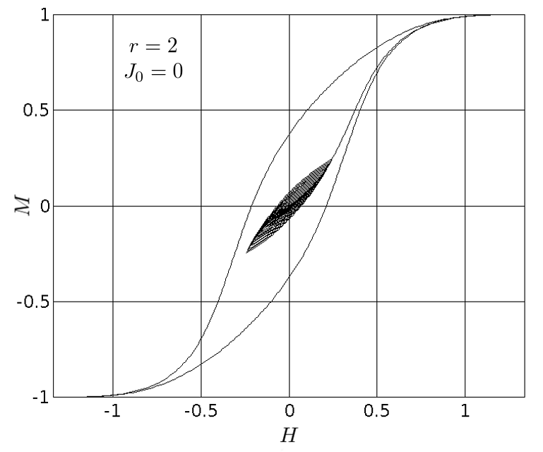
(a)

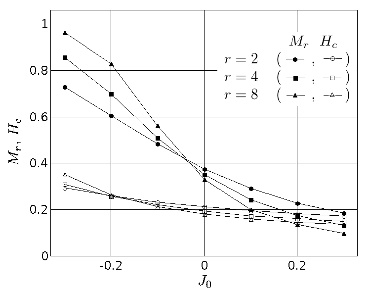
(b)

Figure 2: Main hysteresis loop and a series of symmetric minor loops for $r=2$, $J_{0}=0$ and $\Delta J=1$ (left); Remanence and coercivity for different values of $r$, $J_{0}$, and $\Delta J=1$ (right).

The deterministic rules describing the dynamics of the model were used. When the field changes, the stability of spins is checked in the order of numbering. The first unstable spin flips and the neighboring sites are updated and checked; again, the first unstable spin flips and its neighboring sites are updated, and so on, until the spins in the group become stable. Then the remaining spins are checked and flipped in the same way, until all the spins are in the stable state. Another dynamics with random selection between the unstable spins was tested, with no noticeable difference in the shape of hysteresis curves.

In the region $-0.3\leq J_{0}\leq 0.3$ the hysteresis curves are comparable to those of ferromagnets, as shown in Fig. 2. The behavior of the model was studied in this interval of $J_{0}$. The model demonstrates noticeable but not very significant deviations from the macroscopic RPM. The deviations from the microscopic RPM are as follows. For $J_{0}=0,r=2$, RPM holds with accuracy $0.2\%$ for $M_{m}=0.2$, and with accuracy $4\%$ for $M_{m}=0.6$. Deviation from RPM increases with $r$; for $r=8$, about $9\%$ of spins change orientation after completing the symmetric hysteresis cycle with $M_{m}=0.6$.

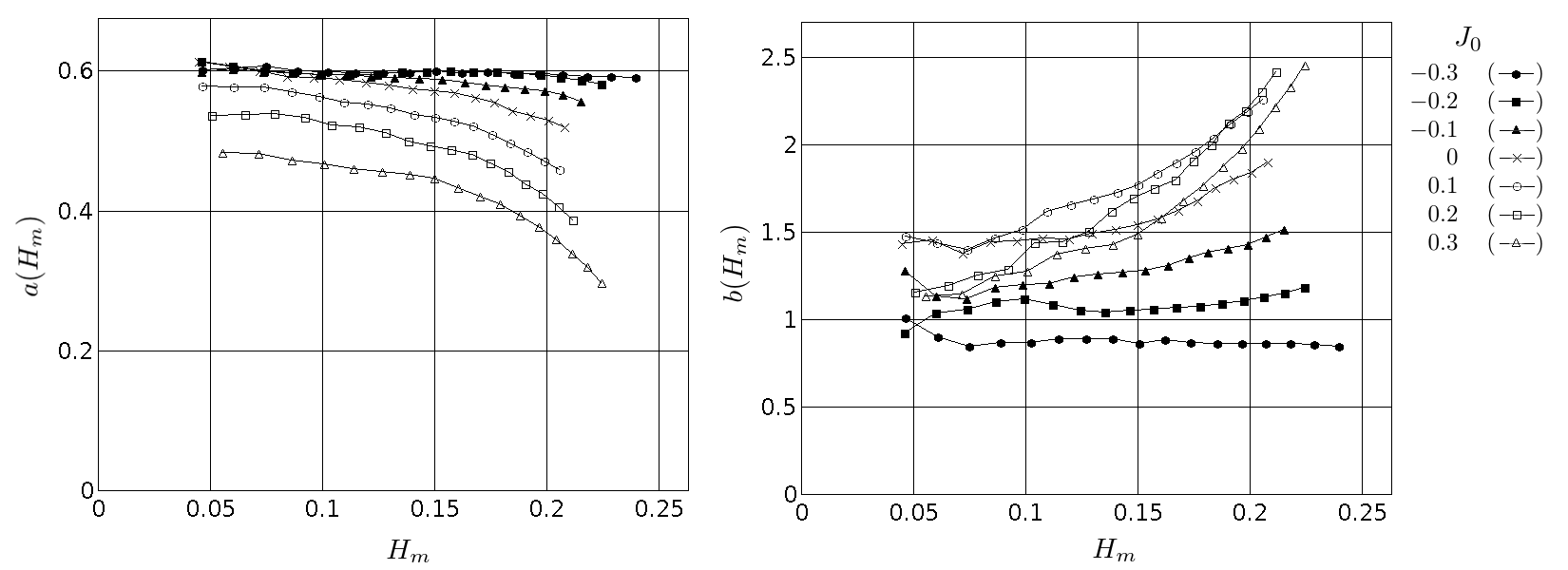
Figure 3: Rayleigh coefficients $a(H_{m})$, $b(H_{m})$ defined according to (21). Parameters of the model are $\Delta J=1$, $r=2$, $J_{0}=-0.3\,\ldots\,0.3$, $N=2\cdot 10^{5}$.

For the experiments in the neighborhood of the demagnetized state were taken $N=2\cdot 10^{5}$, $r=2$. The demagnetized state was obtained by applying a series of cycles, each one with the maximum magnetization equal to the maximum magnetization of the previous cycle multiplied by a constant coefficient $k<1$ selected close to $1$. This procedure provides fine demagnetization near the demagnetized sate, while for large $H$ the demagnetization is relatively coarse.

Parameters $a(H_{m}),\,b(H_{m})$ defined according to (21) are presented in Fig. 3. Irregular behavior of the curves could be explained by insufficient value of $N$, not fine enough demagnetization, or imperfections of the random number generator. The irregular run of the curves in Fig. 3 do not allow to make a conclusion on applicability of equations (22).

For the values of $H_{m}$ where the Rayleigh equations (1) hold true, $a(H_{m})$, $b(H_{m})$ must be equal to the Rayleigh constants $a$, $b$. Not taking into account the irregularity of the curves in Fig. 3, it can be expected that for $J_{0}=-0.3$ and for $J_{0}=-0.2$ the Rayleigh approximation (1) is applicable, with some accuracy, up to $H_{m}=0.2$. It is unclear whether the Rayleigh region is obtained or not for $J_{0}=0.2$ and $J_{0}=0.3$.

Energy Transformations

A consideration similar to that performed in Chapter 5 can be applied to Ising spins, assuming that $Q$ denotes the energy loss instead of the dissipated heat. Therefore, we can expect that equation (29) holds true in the region of fields where the Rayleigh law is applicable.

The curves with $H_{m}<0.8$ were abandoned as not reliable. For $J_{0}=-0.2$, $J_{0}=-0.3$, and $0.08\leq H_{m}\leq 0.22$, equations (1), (29) agree with the experiment as shown in Fig. 4 as an example. The model gives similar plots starting from $H_{m}\approx 0.08$ for all examined values of $J_{0}$. While $H_{m}$ increases, the disagreement becomes noticeable first with (29) and later with (1). For $J_{0}=0.3$, relatively small disagreement between (29) and the experiment is observed at $H_{m}=0.1$, the disagreement with (1) becomes apparent after $H_{m}=0.15$.

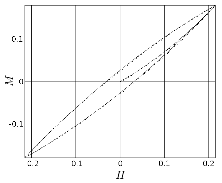
(a)

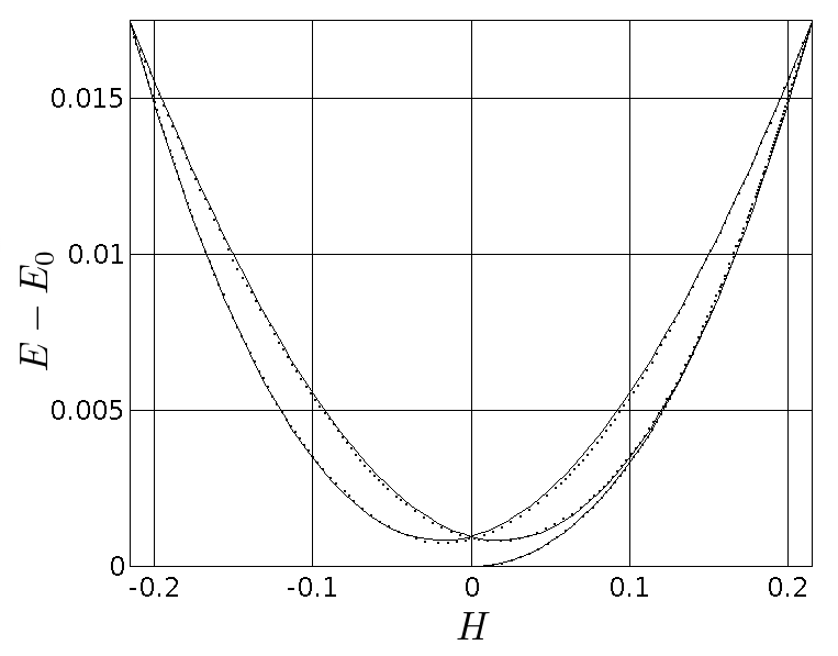
(b)

Figure 4: Rayleigh hysteresis loop in $H,M$ and $H,E$ coordinates; $J_{0}=-0.2$, $\Delta J=1$, $r=2$, and $H_{m}\approx 0.21$. Dotted curves represent the result of the numerical experiment on RBIM, solid ones are calculated according to equations (1), (29) with the same Rayleigh constants, by letting $a=a(H_{m})$, $b=b(H_{m})$.

7 Conclusions

The sequences of polynomials $\{P^{(k)}_{n}(\xi_{0},\ldots,\xi_{n})\}$ that are consistent with the return point memory and the reachability of the demagnetized state must satisfy conditions (Y0) – (Y2). These polynomials can be used for Taylor expansion of the whole set of hysteresis curves in the neighborhood of the demagnetized state. Eight sequences of polynomials listed in Table 1 form a basis in the linear space of the sequences of polynomials up to the third degree.

There are only two antisymmetric polynomials up to the second degree in the basis, and a linear combination of them (17) gives the Rayleigh law. Antisymmetric polynomials of the third degree add two terms to the Rayleigh law according to equations (19), (20).

Equation (28) describing dependence of the energy on the magnetic state $(\xi_{0},\ldots,\xi_{n})$ were derived from the following assumptions: (i) the hysteresis curves comply with the Rayleigh law according to (18), and (ii) the heat is always dissipated when the magnetic state changes. For symmetric hysteresis cycles equation (28) gives the dependence of the energy on the applied magnetic field in the Rayleigh-like form (29).

Equations (28), (29) have no adjustable parameters but are applicable only to hysteresis systems without the magnetocaloric effect. In general case, they are not applicable to real ferromagnets. However, these equations must presumably agree with hysteresis models that show the return point memory, have smooth hysteresis curves, and can be demagnetized by an alternating magnetic field. Numerical results obtained in the random bond Ising model show reasonable agreement with equation (29).

References

[1]
G. Bertotti.
Hysteresis in Magnetism (for physicists, materials scientists,
and engineers).
Academic Press, Boston, 1998.
[2]
R. M. Bozorth.
Ferromagnetism.
D. Van Nostrand Company, Inc., Toronto - New York - London, 1951.
[3]
S. Chikazumi.
Physics of Ferromagnetism.
Clarendon Press, Oxford, 1997.
[4]
F. Colaiori, A. Gabrielli, and S. Zapperi.
Rayleigh loops in the random-field Ising model on the Bethe
lattice.
Phys. Rev. B, 65(224404), 2002.
[5]
B. D. Cullity and C. D. Graham.
Introduction to Magnetic Materials.
IEEE Press, 2009.
[6]
L. Dante, G. Durin, A. Magni, and S. Zapperi.
Low field hysteresis in disordered ferromagnets.
Phys. Rev. B, 65(144441), 2002.
[7]
H. G. Katzgrabber, F. Pázmándi, C. R. Pike, K. Liu, R. T. Scalett,
K. L. Verosub, and G. T. Zimányi.
Reversal-field memory in magnetic hysteresis.
J. Appl. Phys., 93(10):6617, 2003.
[8]
S. E. Langvagen.
State-space representation of hysteresis systems exhibiting the
return point memory.
arXiv:1701.00727 [math.DS], 2017.
[9]
I. D. Mayergoyz.
Mathematical Models of Hysteresis and Their Applications: Second
Edition.
Electriomagnetism. Academic Press, 2003.
[10]
L. Neel.
Théorie des lois d’aimantation de Lord Rayleigh. I: Les
déplacements d’une paroi isolée.
Cahiers de Phys., 12:1–20, 1942.
[11]
L. Neel.
Théorie des lois d’aimantation de Lord Rayleigh. II:
Multiples domaines et champ coercitif.
Cahiers de Phys., 13:18–30, 1943.
[12]
J. Ortin and J. Goicoechea.
Dissipation in quasistatically driven disordered systems.
Phys. Rev. B, 58(9):5628 – 5631, 1998.
[13]
J. W. S. Rayleigh.
On the behaviour of iron and steel under the operation of feeble
magnetic forces.
Phil. Mag., 23:225–245, 1887.
[14]
J. P. Sethna, K. Dahmen, S. Kartha, J. A. Krumhansl, B. W. Roberts, and J. D.
Shore.
Hysteresis and hierarchies: dynamics of disorder-driven first-order
phase transformations.
Phys. Rev. Lett., 70:3347–3350, 1993.
[15]
E. Vives and A. Planes.
Avalanches in a fluctuationless first-order phase transition in a
random-bond Ising model.
Phys. Rev. B, 50(6):3839–3848, 1994.
[16]
S. Zapperi, A. Magni, and G. Durin.
Microscopic foundations of the Rayleigh law of hysteresis.
JMMM, 242-245 P2:987–992, 2002.