Exploring the nonlinear regime of light-matter interaction using electronic spins in diamond

Abstract

The coupling between defects in diamond and a superconducting microwave resonator is studied in the nonlinear regime. Both negatively charged nitrogen-vacancy and P1 defects are explored. The measured cavity mode response exhibits strong nonlinearity near a spin resonance. Data is compared with theoretical predictions and a good agreement is obtained in a wide range of externally controlled parameters. The nonlinear effect under study in the current paper is expected to play a role in any cavity-based magnetic resonance imaging technique and to impose a fundamental limit upon its sensitivity.

Cavity quantum electrodynamics (CQED) Haroche and Kleppner (1989) is the study of the interaction between photons confined in a cavity and matter. CQED has applications in a variety of fields, including magnetic resonance imaging and quantum computation Wallraff et al. (2004). The CQED interaction can be probed by measuring the response of a cavity mode. Commonly, the effect of matter on the response diminishes as the energy stored in the cavity mode under study is increased Anders (2018). This nonlinear effect, which is the focus of the current study, imposes a severe limit upon the performance of a variety of CQED systems.

In the current study we explore nonlinear CQED interaction between defects in a diamond crystal and a superconducting microwave cavity (resonator) having a spiral shape Maleeva et al. (2013, 2014). Two types of defects are investigated, a negatively charged nitrogen-vacancy NV^- defect and a nitrogen 14 (nuclear spin 1) substitutional defect (P1). Strong coupling between defects in diamond and a superconducting resonator has been demonstrated at ultra-low temperatures Zhu et al. (2011); Kubo et al. (2010, 2011); Amsüss et al. (2011); Schuster et al. (2010); Sandner et al. (2012); Grezes et al. (2014), however the regime of nonlinear response was not addressed. In this study, we find that the cavity response becomes highly nonlinear near a CQED resonance. In addition, for the case of NV^- defects, the response is strongly affected by applying optically-induced spin polarization (OISP). The experimental findings are compared with theory and good agreement is obtained.

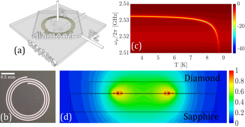
Figure 1: The experimental setup. (a) A loop antenna (LA) is coupled to the spiral resonator. Two multimode optical fibers are coupled to the diamond wafer. Fiber F1 is employed for delivering laser light of wavelength $\lambda_{\mathrm{L}}=532\operatorname{nm}$, and fiber F2 probes the emitted photoluminescence (PL). (b) The spiral resonator has $3$ turns, an inner radius of $0.59\operatorname{mm}$ and an outer radius of $0.79\operatorname{mm}$. (c) The resonance lineshape of the spiral’s fundamental mode vs. temperature. (d) The magnetic induction magnitude $\left|\mathbf{B}_{\mathrm{c}}\left(\mathbf{r}\right)\right|$ of the fundamental mode vs. position $\mathbf{r}$ in a plane perpendicular to both wafers that contains the center of the spiral.

The experimental setup is schematically depicted in Fig. 1(a). Defects in a [100] type Ib diamond are created using $2.8\operatorname{MeV}$ electron irradiation with a dose of approximately $8\times 10^{18}~{}\mathrm{e/cm^{2}}$, followed by annealing at $800^{\circ}\mathrm{C}$ for 8 hours and acid cleaning, resulting in the formation of NV^- defects with density of $1.23\times 10^{17}\operatorname{cm}^{-3}$ Farfurnik et al. (2017). The diamond wafer is then placed on top of a sapphire wafer supporting a superconducting spiral resonator made of niobium [see Fig. 1(b)]. Externally applied magnetic field $\mathbf{B}$ is employed for tuning the system into a CQED resonance. A coaxial cable terminated by a loop antenna (LA) transmits both injected and off-reflected microwave signals. The LA has a coupling given by $\gamma_{\mathrm{f}}/2\pi=0.367\operatorname{MHz}$ to the spiral’s fundamental mode, which has a frequency of $\omega_{\mathrm{c}}/2\pi=2.53\operatorname{GHz}$ and an unloaded damping rate of $\gamma_{\mathrm{c}}/2\pi=0.253\operatorname{MHz}$ [these values are extracted from a fitting based on Eq. (7) below]. All measurements are performed at a base temperature of $T=3.1\operatorname{K}$. A network analyzer (NA) measurement of the temperature dependence of the resonance lineshape is seen in Fig. 1(c). The color-coded plot depicts the reflectivity coefficient $R_{\mathrm{c}}=P_{\mathrm{r}}/P_{\mathrm{p}}$ is dB units, where $P_{\mathrm{p}}=-70$ dBm and $P_{\mathrm{r}}$ are, respectively, the injected power into the LA and the off-reflected power from the LA, as a function of both frequency of injected signal $\omega_{\mathrm{p}}/2\pi$ and temperature $T$. Laser light of wavelength $\lambda_{\mathrm{L}}=532\operatorname{nm}$ and intensity $I_{\mathrm{L}}$ (in units of power per unit area) is injected into the diamond wafer using a multimode optical fiber F1, and another multimode optical fiber F2 delivers the emitted photoluminescence (PL) to an optical spectrum analyzer [see Fig. 2(a)]. Numerical calculation is employed for evaluating the shape of the spiral’s fundamental mode [see Fig. 1(d)].

The negatively-charged $\text{NV}^{-}$ defect in diamond consists of a substitutional nitrogen atom (N) combined with a neighbor vacancy (V) Doherty et al. (2013). The ground state of the NV^- defect is a spin triplet having symmetry ${}^{3}A_{2}$ Maze et al. (2011); Wrachtrup and Jelezko (2006), composed of a singlet state $\left|m_{\mathrm{e}}=0\right\rangle$ and a doublet $\left|m_{\mathrm{e}}=\pm 1\right\rangle$. The angular resonance frequencies $\omega_{\pm}$ corresponding to the transitions between the state $\left|m_{\mathrm{e}}=0\right\rangle$ and the states $\left|m_{\mathrm{e}}=\pm 1\right\rangle$ are approximately given by Ovartchaiyapong et al. (2014); MacQuarrie et al. (2013); Rondin et al. (2014)

$$\omega_{\pm}=D\pm\sqrt{\gamma_{\mathrm{e}}^{2}B_{\parallel}^{2}+E^{2}}+\frac{3}{2}\frac{\gamma_{\mathrm{e}}^{2}B_{\perp}^{2}}{D}\;,$$ (1)

where $B_{\parallel}$ is the magnetic field component parallel to the axis of the NV defect and $B_{\perp}$ is the transverse one. The parameter $\gamma_{\mathrm{e}}=2\pi\times 28.03\operatorname{GHz}\operatorname{T}^{-1}$ is the electron spin gyromagnetic ratio. In the absence of strain and when the externally applied magnetic field vanishes one has $\omega_{\pm}=D$, where $D=2\pi\times 2.87\operatorname{GHz}$. Internal strain, however, may lift the degeneracy between the states $\left|m_{\mathrm{e}}=-1\right\rangle$ and $\left|m_{\mathrm{e}}=+1\right\rangle$, and give rise to a splitting given by $2E$ (in our sample $E=2\pi\times 10\operatorname{MHz}$). In a single crystal diamond the NV defects have four different possible orientations with four corresponding pairs of angular resonance frequencies $\omega_{\pm}$.

The technique of optical detection of magnetic resonance (ODMR) can be employed for measuring the resonance frequencies $\omega_{\pm}$ Gruber et al. (1997); Le Sage et al. (2012). The measured PL spectrum is seen in Fig. 2(a). The integrated PL signal in the band $660\operatorname{nm}-760\operatorname{nm}$ is plotted as a function of microwave input frequency $\omega_{\mathrm{p}}/2\pi$ and externally applied magnetic field $\left|\mathbf{B}\right|$ in Figs. 2(b)-(c). In this measurement the microwave input power is set to $P_{\mathrm{p}}=20\;$dBm. The direction of the externally applied magnetic field $\mathbf{B}$ is found by fitting the measured ODMR frequencies $\omega_{\pm}$ with the calculated values given by Eq. (1).

The ODMR spectrum contains a profound resonance feature at the frequency of the spiral resonator $\omega_{\mathrm{c}}/2\pi=2.53\operatorname{GHz}$ [see Fig. 2(b)]. This feature is attributed to heating-induced change in the internal stress in the diamond wafer. Two (out of four) resonance frequencies $\omega_{-}/2\pi$ can be tuned close to the spiral resonator frequency $\omega_{\mathrm{c}}/2\pi$ by setting the magnetic field $\left|\mathbf{B}\right|$ close to the value of $16\operatorname{mT}$. The two groups of NV^- defects giving rise to these two resonances have the smallest angles with respect to the externally applied magnetic field (see caption of Fig. 2). In this region, which is magnified in Fig. 2(c), the deepest ODMR is obtained when the magnetic and resonator frequencies coincide.

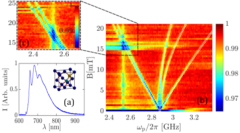
Figure 2: ODMR (a) The measured emitted PL spectrum. (b) and (c) ODMR spectrum vs. driving frequency $\omega_{\mathrm{p}}/2\pi$ and magnetic field $\left|\mathbf{B}\right|$. The white dotted lines represent the frequencies $\omega_{\pm}/2\pi$ calculated using Eq. (1). The fitting procedure yields the direction of the magnetic field $\mathbf{\hat{b}}$, which is expressed as $\mathbf{\hat{b}}=T_{\mathbf{\hat{z}}}\left(\theta_{z}\right)T_{\mathbf{\hat{y}}}\left(\theta_{y}\right)T_{\mathbf{\hat{x}}}\left(\theta_{x}\right)\mathbf{\hat{z}}$, where $\mathbf{\hat{x}}$, $\mathbf{\hat{y}}$ and $\mathbf{\hat{z}}$ are unit vectors in the crystal directions $\left[100\right]$, $\left[010\right]$ and $\left[001\right]$, respectively, and $T_{\mathbf{\hat{s}}}\left(\theta_{s}\right)$ is a rotation operator around the axis $\mathbf{\hat{s}}$, where $s\in\left\{x,y,z\right\}$. The rotation angles found from the fitting procedure are $\theta_{x}/\pi=-0.02$, $\theta_{y}/\pi=0.002$ and $\theta_{z}/\pi=0.05$.

The same two spin resonances seen in Fig. 2(c) can be detected without employing the technique of ODMR provided that their frequencies are tuned close to the spiral resonator frequency $\omega_{\mathrm{c}}/2\pi$. The plots (D: P1; L0), (D: P2; L0) and (D: P3; L0) of Fig. 3 depicts NA measurements of the microwave reflectivity coefficient $R_{\mathrm{c}}$ with three different values of the injected signal microwave power $P_{\mathrm{p}}$. No laser light is injected into the diamond wafer in these measurements (labeled by L0 in Fig. 3). Henceforth this method of spin detection is referred to as cavity-based detection of magnetic resonance (CDMR). Both CDMRs seen in Fig. 3 exhibit strong dependence on $P_{\mathrm{p}}$, indicating thus that the interaction with the spins makes the cavity response highly nonlinear.

To account for the observed spin-induced nonlinearity, the experimental results are compared with theoretical predictions Boissonneault et al. (2008). The decoupled cavity mode is characterized by an angular resonance frequency $\omega_{\mathrm{c}}$, Kerr coefficient $K_{\mathrm{c}}$, linear damping rate $\gamma_{\mathrm{c}}$ and cubic damping (two-photon absorption) rate $G_{\mathrm{c}}$. The response of the decoupled cavity in the weak nonlinear regime (in which, nonlinearity is taken into account to lowest non-vanishing order) can be described by introducing the complex and mode amplitude dependent cavity angular resonance frequency $\Upsilon_{\mathrm{c}}$, which is given by

$$\Upsilon_{\mathrm{c}}=\omega_{\mathrm{c}}-i\gamma_{\mathrm{c}}+\left(K_{\mathrm{c}}-iG_{\mathrm{c}}\right)E_{\mathrm{c}}\;,$$ (2)

where $E_{\mathrm{c}}$ is the averaged number of photons occupying the cavity mode. The imaginary part of $\Upsilon_{\mathrm{c}}$ represents the effect of damping and the terms proportional to $E_{\mathrm{c}}$ represent the nonlinear contribution to the response.

The effect of the spins on the cavity response in the weak nonlinear regime is theoretically evaluated in Buks et al. (2016). The steady state cavity mode response is found to be equivalent to the response of a mode having effective complex cavity angular resonance frequency $\Upsilon_{\mathrm{eff}}$ given by $\Upsilon_{\mathrm{eff}}=\Upsilon_{\mathrm{c}}+\Upsilon_{\mathrm{s}}$, where $\Upsilon_{\mathrm{s}}=\sum_{n}\Upsilon_{n}$ and $\Upsilon_{n}$, which represents the contribution of a spin labeled by the index $n$, is given by [see Eq. (4) in Buks et al. (2016)]

$$\Upsilon_{n}=-\frac{g_{n}^{2}}{\Delta_{n}}\frac{1-\frac{i}{\Delta_{n}T_{2,n}}}{1+\frac{1+4g_{n}^{2}T_{1,n}T_{2,n}E_{\mathrm{c}}}{\Delta_{n}^{2}T_{2,n}^{2}}}P_{z\mathrm{S},n}\;,$$ (3)

where $g_{n}$ is the coupling coefficient between the $n$th spin and the cavity mode, $T_{1,n}$ and $T_{2,n}$ are the spin’s longitudinal and transverse relaxation times, respectively, $\Delta_{n}=\omega_{\mathrm{c}}-\omega_{\mathrm{s},n}$ is the frequency detuning between the cavity frequency $\omega_{\mathrm{c}}$ and the spin’s transition frequency $\omega_{\mathrm{s},n}$, and $P_{z\mathrm{S},n}$ is the spin’s longitudinal polarization. The term proportional to $E_{\mathrm{c}}$ in the denominator of Eq. (3) gives rise to nonlinear response.

The coupling coefficients $g_{n}$ can be extracted from the numerically calculated magnetic field induction $\mathbf{B}_{\mathrm{c}}\left(\mathbf{r}\right)$ of the spiral’s fundamental mode [see Fig. 1(d)] using the expression $g_{n}=\gamma_{\mathrm{e}}\left|\mathbf{B}_{\mathrm{c}}\left(\mathbf{r}_{n}\right)\right|\sin\varphi_{n}/E_{\mathrm{c}}^{1/2}$ Kubo et al. (2010), where $\mathbf{B}_{\mathrm{c}}\left(\mathbf{r}_{n}\right)$ is the cavity mode magnetic induction at the location of the spin $\mathbf{r}_{n}$ and $\varphi_{n}$ is the angle between $\mathbf{B}_{\mathrm{c}}\left(\mathbf{r}_{n}\right)$ and the NV axis. When all contributing spins share the same detuning factor $\Delta$, polarization$P_{z\mathrm{S}}$ and the same relaxation times $T_{1}$ and $T_{2}$, and when the variance in the distribution of $g_{n}$ is taken into account to lowest nonvanishing order only, one finds that

$$\Upsilon_{\mathrm{s}}=\frac{N_{\mathrm{eff}}g_{\mathrm{s}}^{2}}{\Delta}\frac{1-\frac{i}{\Delta T_{2}}}{1+\frac{1+\frac{E_{\mathrm{c}}}{E_{\mathrm{cc}}}}{\Delta^{2}T_{2}^{2}}}{},$$ (4)

where $\rho_{\mathrm{s}}\left(\mathbf{r}\right)$ is the density of contributing NV^- defects, $N_{\mathrm{eff}}=-\int d\mathbf{r}{}\rho_{\mathrm{s}}P_{z\mathrm{S}}$ is their effective number, the effective coupling coefficient $g_{\mathrm{s}}$ is given by

$$g_{\mathrm{s}}^{2}=\frac{\gamma_{\mathrm{e}}^{2}\mu_{0}\hbar\omega_{\mathrm{c}}\int\mathrm{d}\mathbf{r}{}\rho_{\mathrm{s}}\left|\mathbf{B}_{\mathrm{c}}\right|^{2}\sin^{2}\varphi P_{z\mathrm{S}}}{\int\mathrm{d}\mathbf{r}{}\left|\mathbf{B}_{\mathrm{c}}\right|^{2}\int\mathrm{d}\mathbf{r}{}\rho_{\mathrm{s}}P_{z\mathrm{S}}}{},$$ (5)

and $E_{\mathrm{cc}}=\left(4g_{\mathrm{s}}^{2}T_{1}T_{2}\right)^{-1}$.

The underlying mechanism responsible for the spin-induced nonlinearity in the cavity mode response is attributed to the change in spin polarization that occurs via the cavity-mediated spin driving. As can be seen from Eq. (A83) of Ref. Buks et al. (2016), the normalized change in polarization is proportional to the ratio $E_{\mathrm{c}}/E_{\mathrm{cc}}$. Consequently, the induced nonlinearity is expected to be negligibly small when $E_{\mathrm{c}}\ll E_{\mathrm{cc}}$ [as is also seen from Eq. (4)]. On the other hand, when $E_{\mathrm{c}}\gg E_{\mathrm{cc}}$ spin depolarization becomes saturated. In this limit $\Upsilon_{\mathrm{eff}}=\Upsilon_{\mathrm{c}}+\Upsilon_{\mathrm{s}}\simeq\Upsilon_{\mathrm{c}}$ [see Eq. (4)], and consequently the cavity mode is expected to become effectively decoupled from the spins (this effective decoupling refers only to the averaged response, whereas noise properties remain affected by the spins). The regime of weak nonlinearity, in which nonlinearity can be taken into account to lowest nonvanishing order only, is discussed in appendix A. Note, however, that in the current experiment the nonlinearity can be considered as weak only in a narrow region, and most observations cannot be properly explained without accounting for higher order nonlinear terms.

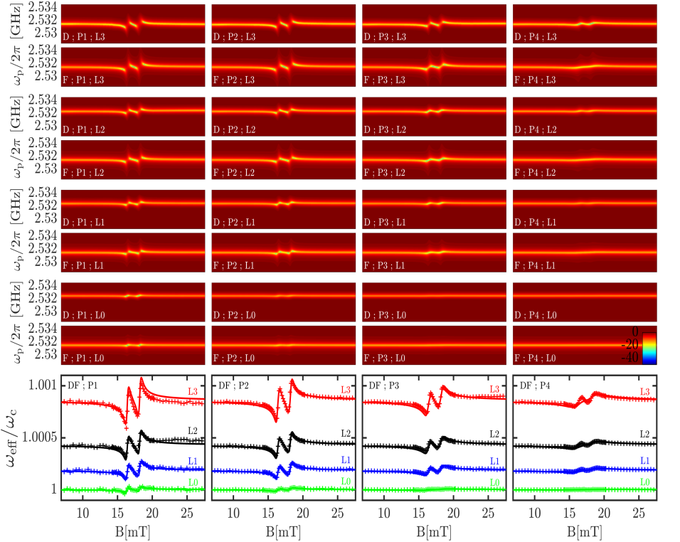
Figure 3: Cavity mode reflectivity $R_{\mathrm{c}}$ with NV^- defects for various values of injected microwave power $P_{\mathrm{p}}$ ($\mathrm{P}1=-90~{}\mathrm{dBm}$, $\mathrm{P}2=-70~{}\mathrm{dBm}$, $\mathrm{P}3=-60~{}\mathrm{dBm}$ and $\mathrm{P}4=-50~{}\mathrm{dBm}$) and laser power $I_{\mathrm{L}}$ ($\mathrm{L}0=0$, $\mathrm{L}1=5.6\operatorname{mW}\operatorname{mm}^{-2}$, $\mathrm{L}2=12.8\operatorname{mW}\operatorname{mm}^{-2}$ and $\mathrm{L}3=30\operatorname{mW}\operatorname{mm}^{-2}$). For each pair the top plot is experimental data (labeled by D) and the bottom is the theoretical prediction (labeled by F). The bottom row shows the effective normalized resonance frequency ($\omega_{\text{eff}}/\omega_{\text{c}}$), which is obtained from the minimum reflectivity signal for each magnetic field, as a function of magnetic field. Each column corresponds to a single microwave power (DF ; P1-P4) and each plot shows all four laser powers (L3 in red, L2 in black, L1 in blue and L0 in green). Cross markers denote experimental data and solid lines represent theoretical predictions. Plots are vertically shifted for clarity. The parameters used for the calculation for the case of laser on (off) are: $P_{z\mathrm{ST}}=-0.035$, $P_{z\mathrm{SO}}=-0.55$, $\rho_{\mathrm{s}}=1.23\times 10^{17}\operatorname{cm}^{-3}$, $T_{2}=219\operatorname{ns}$, $T_{1\mathrm{T}}=23\operatorname{ms}$ ($T_{1\mathrm{T}}=565\operatorname{ms}$) Loretz et al. (2017) and $g_{\mathrm{s}}/2\pi=5.05\operatorname{Hz}$ ($g_{\mathrm{s}}/2\pi=2.72\operatorname{Hz}$). The rate $T_{1\mathrm{O}}^{-1}$ of OISP is taken to be given by $T_{1\mathrm{O}}^{-1}=0.16\times\gamma_{\mathrm{O}}$, where $\gamma_{\mathrm{O}}=I_{\mathrm{L}}\sigma\lambda_{\mathrm{L}}/hc$ is rate of optical absorption, where $\sigma=3\times 10^{-17}\operatorname{cm}^{2}$ Wee et al. (2007) is the optical cross section, $h$ is the Plank’s constant and $c$ is the speed of light in vacuum. The effective coupling coefficient $g_{\mathrm{s}}$ for both cases of laser on and off is calculated using Eq. (5) and the numerically calculated mode shape [see Fig.1 (d)]. The volume inside the diamond wafer illuminated by the laser is $0.76\operatorname{mm}^{3}$.

In general, the averaged number of photons $E_{\mathrm{c}}$ is found from the steady state solution of the equations of motion that govern the dynamics of the system Buks et al. (2016). To lowest non-vanishing order in the coupling coefficient $g_{\mathrm{s}}$ the effect of spins can be disregarded in the calculation of $E_{\mathrm{c}}$. When, in addition, the intrinsic cavity mode nonlinearity, which is characterized by the parameters $K_{\mathrm{c}}$ and $G_{\mathrm{c}}$, has a negligibly small effect, the number $E_{\mathrm{c}}$ can be approximated by the following expression [see Eq. (37) in Yurke and Buks (2006)]

$$E_{\mathrm{c}}=\frac{4\gamma_{\mathrm{f}}P_{\mathrm{p}}}{\hbar\omega_{\mathrm{c}}}\frac{1}{\left(\omega_{\mathrm{p}}-\omega_{\mathrm{c}}\right)^{2}+\left(\gamma_{\mathrm{f}}+\gamma_{\mathrm{c}}\right)^{2}}\;.$$ (6)

As can be seen from Eq. (4), $\left|\Upsilon_{\mathrm{s}}\right|$ is a monotonically decreasing function of $E_{\mathrm{c}}$. This suggests that the approximation in which Eq. (6) is employed for evaluating $E_{\mathrm{c}}$ (without taking into account both nonlinearity and the coupling to the spins) remains valid even when $4g_{\mathrm{s}}^{2}T_{1}T_{2}E_{\mathrm{c}}\gg 1$ provided that intrinsic cavity mode nonlinearity remains sufficiently small. When intrinsic cavity mode nonlinearity can be disregarded the cavity mode reflectivity $R_{\mathrm{c}}$ is given by Yurke and Buks (2006)

$$R_{\mathrm{c}}=\frac{\left(\omega_{\mathrm{p}}-\Omega_{\mathrm{c}}\right)^{2}+\left(\gamma_{\mathrm{f}}-\Gamma_{\mathrm{c}}\right)^{2}}{\left(\omega_{\mathrm{p}}-\Omega_{\mathrm{c}}\right)^{2}+\left(\gamma_{\mathrm{f}}+\Gamma_{\mathrm{c}}\right)^{2}}\ ,$$ (7)

where the real frequencies $\Omega_{\mathrm{c}}$ and $\Gamma_{\mathrm{c}}$ are related to the complex frequency $\Upsilon_{\mathrm{eff}}$ by the relation $\Upsilon_{\mathrm{eff}}=\Omega_{\mathrm{c}}-i\Gamma_{\mathrm{c}}$.

The fully-analytical theoretical predictions given by Eqs. (4), (6) and (7) are employed for generating the plots (F: P1; L0), (F: P2; L0) and (F: P3; L0) of Fig. 3, which exhibit good agreement with the corresponding CDMR data plots (D: P1; L0), (D: P2; L0) and (D: P3; L0). The parameters that have been employed for the calculation are listed in the figure caption. These findings support the hypothesis that the above-discussed spin-induced nonlinearity is the underlying mechanism responsible for the suppression of electron spin resonance (ESR) at relatively high microwave input power $P_{\mathrm{p}}$.

The CDMR data plots in Fig. 3 labeled by L1, L2 and L3 are obtained from measurements with laser intensities $2.15\operatorname{mW}\operatorname{mm}^{-2}$, $12.8\operatorname{mW}\operatorname{mm}^{-2}$ and $30\operatorname{mW}\operatorname{mm}^{-2}$, respectively. As can be seen from the comparison to the plots labeled by L0, in which the laser is turned off, the optical illumination strongly affects the measured cavity response.

The laser-induced change in the cavity response is attributed to the mechanism of OISP Loretz et al. (2017); Drake et al. (2015); Robledo et al. (2011); Redman et al. (1991); Harrison et al. (2006). Spin is conserved in the optical dipole transitions between the triplet ground state ${}^{3}A_{2}$ of NV^- and the triplet first excited state ${}^{3}E$. However, transition from the spin states $m_{\mathrm{e}}=\pm 1$ of ${}^{3}E$ to the ground state is also possible through an intermediate singlet states in a two-steps non-radiative process. Such non-radiative process is also possible for the decay of the state $m_{\mathrm{e}}=0$ of ${}^{3}E$, however, the probability of this process is about $7$ times smaller than the probability of non-radiative decay of the $m_{\mathrm{e}}=\pm 1$ states Doherty et al. (2013). The asymmetry between the decay of $m_{\mathrm{e}}=0$ state, which is almost exclusively radiative, and the decay of the states $m_{\mathrm{e}}=\pm 1$, which can occur via non-radiative process, gives rise to OISP. For our experimental conditions the probability to find any given NV^- defect at any given time not in the triplet ground state ${}^{3}A_{2}$ is about $10^{-5}$ or less Doherty et al. (2013). This fact is exploited below for taking the effect of OISP into account within the framework of a two-level model.

The effect of OISP can be accounted for by adjusting the values of the longitudinal relaxation time $T_{1}$ and longitudinal steady state polarization $P_{z\mathrm{S}}$ and make them dependent on laser intensity $I_{\mathrm{L}}$. The total rate of spin longitudinal damping $\gamma_{\mathrm{s}1}$ is given by Shin et al. (2012)

$$\gamma_{\mathrm{s}1}=-\frac{P_{z}-P_{z\mathrm{ST}}}{T_{1\mathrm{T}}}-\frac{P_{z}-P_{z\mathrm{SO}}}{T_{1\mathrm{O}}}\ ,$$ (8)

where the first term represents the contribution of thermal relaxation and the second one represents the contribution of OISP. Here $P_{z}$ is the instantaneous longitudinal polarization and $T_{1\mathrm{T}}^{-1}$ ($T_{1\mathrm{O}}^{-1}$) is the rate of thermal relaxation (OISP). In steady state and when $T_{1\mathrm{T}}^{-1}\gg T_{1\mathrm{O}}^{-1}$ (i.e. when OISP is negligibly small) the coefficient $P_{z\mathrm{ST}}=-\tanh\left(\hbar\omega_{\mathrm{s}}/2k_{\mathrm{B}}T\right)$ is the value of $P_{z}$ in thermal equilibrium, where $k_{\mathrm{B}}$ is the Boltzmann’s constant and where $T$ is the temperature. In the opposite limit of $T_{1\mathrm{O}}^{-1}\gg T_{1\mathrm{T}}^{-1}$ (i.e. when thermal relaxation is negligibly small) the coefficient $P_{z\mathrm{SO}}$ is the value of $P_{z}$ in steady state. Note that the total longitudinal damping rate $\gamma_{\mathrm{s}1}$ (8) can be expressed as $\gamma_{\mathrm{s}1}=-T_{1}^{-1}\left(P_{z}-P_{z\mathrm{S}}\right)$, where $T_{1}^{-1}=T_{1\mathrm{T}}^{-1}+T_{1\mathrm{O}}^{-1}$ is the effective longitudinal relaxation rate, and the effective steady state longitudinal polarization $P_{z\mathrm{S}}$ is given by $T_{1}^{-1}P_{z\mathrm{S}}=T_{1\mathrm{T}}^{-1}P_{z\mathrm{ST}}+T_{1\mathrm{O}}^{-1}P_{z\mathrm{SO}}$.

The theoretical expressions given above for $T_{1}^{-1}$ and $P_{z\mathrm{S}}$ are employed for generating the plots labeled by F of Fig. 3 for both cases of laser off (L0) and laser on (L1, L2 and L3). In spite of the simplicity of the model that is employed for the description of OISP, good agreement is obtained from the comparison with the CDMR data plots labeled by D in a very wide range of values for the microwave power and laser intensity (the entire explored range of $P_{\mathrm{p}}<0$ dBm and $I_{\mathrm{L}}<30\operatorname{mW}\operatorname{mm}^{-2}$). Note that no resonance splitting is observed in all CDMR measurements.

The lineshapes of both ODMR and CDMR depend on the values of spin longitudinal $T_{1}$ and transverse $T_{2}$ damping times. In order to check consistency we employ Eq. (2) of Ref. Jensen et al. (2013) in order to express the full width at half minimum (FWHM) $\Delta\nu$ of the ODMR in terms of $T_{1}$, $T_{2}$ and the driving amplitude, which is denoted by $\omega_{1}$ ($\omega_{1}$ coincides with the Rabi frequency at resonance). In the calculation of $\omega_{1}$ it is assumed that the loop antenna can be treated as a perfect magnetic dipole. By substituting the damping times $T_{1}$ and $T_{2}$ that are listed in the caption of Fig. 3 into Eq. (2) of Ref. Jensen et al. (2013) one obtains $\Delta\nu=14\operatorname{MHz}$, whereas the FWHM value extracted from the ODMR data using a fit to a Lorentzian is $13.5\operatorname{MHz}$.

A CQED resonance due to P1 defects Kaiser and Bond (1959); Smith et al. (1959) is observed when the externally applied magnetic field is tuned close to the value of $89\operatorname{mT}$ (see Fig. 4). When both nuclear Zeeman shift and nuclear quadrupole coupling are disregarded, the spin Hamiltonian of a P1 defect is given by Loubser and van Wyk (1978); Schuster et al. (2010); Wood et al. (2016) $\mathcal{H}=\gamma_{\mathrm{e}}\mathbf{B}\cdot\mathbf{S}+\hbar^{-1}A_{\perp}\left(S_{x}I_{x}+S_{y}I_{y}\right)+\hbar^{-1}A_{\parallel}S_{z}I_{z}$, where $\mathbf{S}=\left(S_{x},S_{y},S_{z}\right)$ is an electronic spin 1/2 vector operator, $\mathbf{I}=\left(I_{x},I_{y},I_{z}\right)$ is a nuclear spin 1 vector operator, $A_{\parallel}=2\pi\times 114.03\operatorname{MHz}$ and $A_{\perp}=2\pi\times 81.33\operatorname{MHz}$ are respectively the longitudinal and transverse hyperfine parameters, and the $z$ direction corresponds to the diamond $\left\langle 111\right\rangle$ axis. When the externally applied magnetic field $\mathbf{B}$ is pointing close to a crystal direction $\left\langle 100\right\rangle$, i.e. when $\cos^{2}\theta\simeq 1/3$, the electron spin resonance at angular frequency $\gamma_{\mathrm{e}}B$ is split due to the interaction with the nuclear spin into three resonances, corresponding to three transitions, in which the nuclear spin magnetic quantum number is conserved. To first order in perturbation theory the angular resonance frequencies are given by $\gamma_{\mathrm{e}}B-\omega_{\mathrm{en}}$, $\gamma_{\mathrm{e}}B$ and $\gamma_{\mathrm{e}}B+\omega_{\mathrm{en}}$, where $\omega_{\mathrm{en}}^{2}=A_{\parallel}^{2}\cos^{2}\theta+A_{\perp}^{2}\sin^{2}\theta$. For the case where $\cos^{2}\theta=1/3$ the calculated splitting is given by $\omega_{\mathrm{en}}/2\pi=93.5\operatorname{MHz}$, whereas the value extracted from the data seen in Fig. 4 is $93.82\operatorname{MHz}$. The plots labeled by F in Fig. 4 represent the theoretical prediction based on the analytical expressions (4), (6) and (7). The comparison with the CDMR data plots (labeled by D) yields a good agreement. The parameters that have been employed for the calculation are listed in the figure caption.

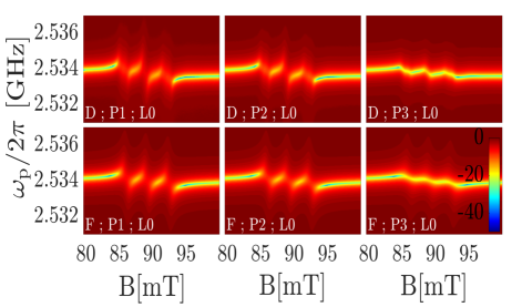
Figure 4: Cavity mode reflectivity $R_{\mathrm{c}}$ with P1 defects for various values of injected microwave power $P_{\mathrm{p}}$ ($\mathrm{P}1=-90~{}\mathrm{dBm}$, $\mathrm{P}2=-80~{}\mathrm{dBm}$ and $\mathrm{P}3=-70~{}\mathrm{dBm}$) with laser off. For each pair the top plot is experimental data (labeled by D) and the bottom is the theoretical prediction (labeled by F). The parameters used for the calculation are: $\gamma_{\mathrm{c}}/2\pi=0.304\operatorname{MHz}$, $\gamma_{\mathrm{f}}/2\pi=0.349\operatorname{MHz}$, $\rho_{\mathrm{s}}=1\times 10^{18}\operatorname{cm}^{-3}$, $T_{2}=438\operatorname{ns}$ and $T_{1\mathrm{T}}=470\operatorname{ms}$ Reynhardt et al. (1998). The values of $P_{z\mathrm{ST}}$ and $g_{\mathrm{s}}$ are the same as in Fig. 3 for the case of laser off.

The nonlinearity in cavity response has an important impact on sensitivity of spin detection. Let $S_{\mathrm{N}}$ be the minimum detectable change in the number of spins $\delta N_{\mathrm{s}}$ per a given square root of the available bandwidth (i.e. the inverse of the averaging time). It is assumed that sensitivity is limited by the fundamental bound imposed upon the signal to noise ratio by shot noise. When the cavity’s response is linear $S_{\mathrm{N}}$ is proportional to $E_{\mathrm{c}}^{-1/2}$ [see Eq. (1) in Buks et al. (2007)], and thus in this regime sensitivity can be enhanced by increasing the energy stored in the cavity $E_{\mathrm{c}}\hbar\omega_{\mathrm{c}}$. However, nonlinearity, which can be avoided only when $E_{\mathrm{c}}\ll E_{\mathrm{cc}}$ [see Eq. (4)], imposes a bound upon sensitivity enhancement. When the sensitivity coefficient $S_{\mathrm{N}}$ is calculated according to Eq. (1) in Ref. Buks et al. (2007) for the case where the number of cavity photons is taken to be $E_{\mathrm{cc}}$ and the responsivity is calculated using Eq. (11) below, one finds that $S_{\mathrm{N}}$ becomes

$$S_{\mathrm{N}}\simeq\frac{2}{\left|P_{z\mathrm{ST}}\right|^{3/2}}\left(\frac{\gamma_{\mathrm{c}}}{g_{\mathrm{s}}^{2}}\frac{2T_{1}}{T_{2}}\right)^{1/2}\ .$$ (9)

Note that in general $2T_{1}/T_{2}\geq 1$ [see Eq. (A79) in Buks et al. (2016)]. For example, for the parameters of our device with laser off Eq. (9) yields $S_{\mathrm{N}}=5\times 10^{7}\operatorname{Hz}^{-1/2}$. The estimate given by Eq. (9) is expected to be applicable for any cavity-based technique of spin detection.

To conclude, in this work we have observed strong coupling (i.e. cooperativity larger than unity) between a superconducting microwave cavity and spin ensembles in diamond (the measured values of the cooperativity parameter $N_{\mathrm{eff}}g_{\mathrm{s}}^{2}/\gamma_{\mathrm{c}}\gamma_{2}$ are $14$ with the NV^- ensemble and laser intensity of $30\operatorname{mW}\operatorname{mm}^{-2}$ and $6.2$ with the P1 ensemble). We find that the coupling imposes an upper bound upon the input microwave power, for which the cavity response remains linear. This bound has important implications on the sensitivity of traditional spin detection protocols that are based on linear response. On the other hand, in some cases nonlinearity can be exploited for sensitivity enhancement (e.g. by generating parametric amplification). However, further study is needed to explore ways of optimizing the performance of sensors operating in the nonlinear regime.

We thank Adrian Lupascu for useful discussions. This work is supported by the Israeli Science Foundation and the Binational Science Foundation.

Appendix A Weak Nonlinearity

In the weak nonlinear regime it is assumed that the averaged number of cavity mode photons $E_{\mathrm{c}}$ is sufficiently small to allow taking nonlinearity into account to lowest non-vanishing order only. In this limit the cavity mode has a nonlinear response that can be adequately described using the well-known Duffing/Kerr model Roy and Devoret (2016). However, as is discussed below, when higher order terms in $E_{\mathrm{c}}$ become significant the response can no longer be described by the Duffing/Kerr model. The distinction becomes most pronounced in the limit of high input microwave power. Both our experimental (see Figs. 3 and 4) and theoretical [see Eq. (4)] results indicate that the cavity mode becomes effectively decoupled from the spins in the limit of high microwave power. Consequently linearity is restored at high input power, provided that the input power is not made too high and it is kept below the region where intrinsic cavity mode nonlinearity, which is characterized by the intrinsic Kerr coefficient $K_{\mathrm{c}}$ and intrinsic cubic damping rate $G_{\mathrm{c}}$, becomes significant. Note that in our device the intrinsic nonlinearity becomes noticeable only when the input power exceeds a value of about $0$ dBm, which is 5-6 orders of magnitude higher than the value at which the cavity becomes effectively decoupled from the spins.

To first order in $E_{\mathrm{c}}$ the spin-induced shift $\Upsilon_{\mathrm{s}}$ in the complex cavity mode angular frequency can be expanded as [see Eq. (4)]

$$\Upsilon_{\mathrm{s}}=\omega_{\mathrm{cs}}-i\gamma_{\mathrm{cs}}+\left(K_{\mathrm{cs}}-iG_{\mathrm{cs}}\right)E_{\mathrm{c}}+O\left(E_{\mathrm{c}}^{2}\right){},$$ (10)

where the shift in linear frequency $\omega_{\mathrm{cs}}$ and the Kerr coefficient $K_{\mathrm{cs}}$ are given by

$$\omega_{\mathrm{cs}} =\frac{N_{\mathrm{eff}}g_{\mathrm{s}}^{2}}{\Delta}\frac{1}{1+\zeta_{2}^{2}}{},$$ (11)

$$K_{\mathrm{cs}} =-\frac{N_{\mathrm{eff}}g_{\mathrm{s}}^{2}}{\Delta E_{\mathrm{cc}}}\left(\frac{\zeta_{2}}{1+\zeta_{2}^{2}}\right)^{2}{},$$ (12)

the linear damping rate is given by $\gamma_{\mathrm{cs}}=\zeta_{2}\omega_{\mathrm{cs}}$ and the cubic damping rate is given by $G_{\mathrm{cs}}=\zeta_{2}K_{\mathrm{cs}}$, and where $\zeta_{2}=1/\Delta T_{2}$. In the regime of linear response (i.e. when $\Upsilon_{\mathrm{s}}=\omega_{\mathrm{cs}}-i\gamma_{\mathrm{cs}}$) Eq. (10) reproduces well-known results for spin-induced frequency shift and broadening of the cavity resonance Haroche and Kleppner (1989). The validity conditions for Eqs. (4) and (10) are discussed in Ref. Buks et al. (2016).

In general, in the weak nonlinear regime, in which higher order terms in $E_{\mathrm{c}}$ can be disregarded, the terms proportional to $E_{\mathrm{c}}$ in the complex angular frequency shift $\Upsilon_{\mathrm{s}}$ [see Eq. (10)] may give rise to bistability in the response of the system to an applied monochromatic driving. At the onset of bistability the averaged number $E_{\mathrm{c}}$ obtains a value denoted by $E_{\mathrm{co}}$. When the value of $E_{\mathrm{co}}$ is estimated based on the assumption that higher order terms in $E_{\mathrm{c}}$ may be disregarded one finds for the parameters of our device that $E_{\mathrm{co}}\simeq 2E_{\mathrm{cc}}$ (calculated using Eq. (42) in Ref. Yurke and Buks (2006)). On the other hand, the assumption that higher order terms in $E_{\mathrm{c}}$ may be disregarded is applicable only when $E_{\mathrm{c}}\ll E_{\mathrm{cc}}$, and thus the nonlinearity cannot be considered as weak in this region. When the bistability is accessible the system can be used for signal amplification Roy and Devoret (2016), which can yield a significant gain close to the onset of bistability Yurke and Buks (2006).

References

- Haroche and Kleppner (1989) S. Haroche and D. Kleppner, Phys. Today 42, 24 (1989).
- Wallraff et al. (2004) A. Wallraff, D. I. Schuster, A. Blais, L. Frunzio, R.-S. Huang, J. Majer, S. Kumar, S. M. Girvin, and R. J. Schoelkopf, Nature 431, 162 (2004).
- Anders (2018) J. Anders, in Recent Advances in Nonlinear Dynamics and Synchronization (Springer, 2018), pp. 57–87.
- Maleeva et al. (2013) N. Maleeva, M. Fistul, A. Averkin, A. Karpov, and A. Ustinov, Proceedings of Metamaterials pp. 474–477 (2013).
- Maleeva et al. (2014) N. Maleeva, M. Fistul, A. Karpov, A. Zhuravel, A. Averkin, P. Jung, and A. Ustinov, Journal of Applied Physics 115, 064910 (2014).
- Zhu et al. (2011) X. Zhu, S. Saito, A. Kemp, K. Kakuyanagi, S.-i. Karimoto, H. Nakano, W. J. Munro, Y. Tokura, M. S. Everitt, K. Nemoto, et al., Nature 478, 221 (2011).
- Kubo et al. (2010) Y. Kubo, F. Ong, P. Bertet, D. Vion, V. Jacques, D. Zheng, A. Dréau, J.-F. Roch, A. Auffèves, F. Jelezko, et al., Physical review letters 105, 140502 (2010).
- Kubo et al. (2011) Y. Kubo, C. Grezes, A. Dewes, T. Umeda, J. Isoya, H. Sumiya, N. Morishita, H. Abe, S. Onoda, T. Ohshima, et al., Physical review letters 107, 220501 (2011).
- Amsüss et al. (2011) R. Amsüss, C. Koller, T. Nöbauer, S. Putz, S. Rotter, K. Sandner, S. Schneider, M. Schramböck, G. Steinhauser, H. Ritsch, et al., Phys. Rev. Lett. 107, 060502 (2011).
- Schuster et al. (2010) D. Schuster, A. Sears, E. Ginossar, L. DiCarlo, L. Frunzio, J. Morton, H. Wu, G. Briggs, B. Buckley, D. Awschalom, et al., Physical review letters 105, 140501 (2010).
- Sandner et al. (2012) K. Sandner, H. Ritsch, R. Amsüss, C. Koller, T. Nöbauer, S. Putz, J. Schmiedmayer, and J. Majer, Physical Review A 85, 053806 (2012).
- Grezes et al. (2014) C. Grezes, B. Julsgaard, Y. Kubo, M. Stern, T. Umeda, J. Isoya, H. Sumiya, H. Abe, S. Onoda, T. Ohshima, et al., Physical Review X 4, 021049 (2014).
- Farfurnik et al. (2017) D. Farfurnik, N. Alfasi, S. Masis, Y. Kauffmann, E. Farchi, Y. Romach, Y. Hovav, E. Buks, and N. Bar-Gill, Applied Physics Letters 111, 123101 (2017).
- Doherty et al. (2013) M. W. Doherty, N. B. Manson, P. Delaney, F. Jelezko, J. Wrachtrup, and L. C. Hollenberg, Physics Reports 528, 1 (2013).
- Maze et al. (2011) J. Maze, A. Gali, E. Togan, Y. Chu, A. Trifonov, E. Kaxiras, and M. Lukin, New Journal of Physics 13, 025025 (2011).
- Wrachtrup and Jelezko (2006) J. Wrachtrup and F. Jelezko, Journal of Physics: Condensed Matter 18, S807 (2006).
- Ovartchaiyapong et al. (2014) P. Ovartchaiyapong, K. W. Lee, B. A. Myers, and A. C. B. Jayich, arXiv:1403.4173 (2014).
- MacQuarrie et al. (2013) E. MacQuarrie, T. Gosavi, N. Jungwirth, S. Bhave, and G. Fuchs, Physical review letters 111, 227602 (2013).
- Rondin et al. (2014) L. Rondin, J. Tetienne, T. Hingant, J. Roch, P. Maletinsky, and V. Jacques, Reports on Progress in Physics 77, 056503 (2014).
- Gruber et al. (1997) A. Gruber, A. Dräbenstedt, C. Tietz, L. Fleury, J. Wrachtrup, and C. Von Borczyskowski, Science 276, 2012 (1997).
- Le Sage et al. (2012) D. Le Sage, L. M. Pham, N. Bar-Gill, C. Belthangady, M. D. Lukin, A. Yacoby, and R. L. Walsworth, Physical Review B 85, 121202 (2012).
- Boissonneault et al. (2008) M. Boissonneault, J. Gambetta, and A. Blais, Physical Review A 77, 060305 (2008).
- Buks et al. (2016) E. Buks, C. Deng, J.-L. F. X. Orgazzi, M. Otto, and A. Lupascu, Phys. Rev. A 94, 033807 (2016).
- Loretz et al. (2017) M. Loretz, H. Takahashi, T. Segawa, J. Boss, and C. Degen, Physical Review B 95, 064413 (2017).
- Wee et al. (2007) T.-L. Wee, Y.-K. Tzeng, C.-C. Han, H.-C. Chang, W. Fann, J.-H. Hsu, K.-M. Chen, and Y.-C. Yu, The Journal of Physical Chemistry A 111, 9379 (2007).
- Yurke and Buks (2006) B. Yurke and E. Buks, J. Lightwave Tech. 24, 5054 (2006).
- Drake et al. (2015) M. Drake, E. Scott, and J. Reimer, New Journal of Physics 18, 013011 (2015).
- Robledo et al. (2011) L. Robledo, H. Bernien, T. van der Sar, and R. Hanson, New Journal of Physics 13, 025013 (2011).
- Redman et al. (1991) D. Redman, S. Brown, R. Sands, and S. Rand, Physical review letters 67, 3420 (1991).
- Harrison et al. (2006) J. Harrison, M. Sellars, and N. Manson, Diamond and related materials 15, 586 (2006).
- Shin et al. (2012) C. S. Shin, C. E. Avalos, M. C. Butler, D. R. Trease, S. J. Seltzer, J. P. Mustonen, D. J. Kennedy, V. M. Acosta, D. Budker, A. Pines, et al., Journal of Applied Physics 112, 124519 (2012).
- Jensen et al. (2013) K. Jensen, V. Acosta, A. Jarmola, and D. Budker, Physical Review B 87, 014115 (2013).
- Kaiser and Bond (1959) W. Kaiser and W. Bond, Physical Review 115, 857 (1959).
- Smith et al. (1959) W. Smith, P. Sorokin, I. Gelles, and G. Lasher, Physical Review 115, 1546 (1959).
- Loubser and van Wyk (1978) J. Loubser and J. van Wyk, Reports on Progress in Physics 41, 1201 (1978).
- Wood et al. (2016) J. D. Wood, D. A. Broadway, L. T. Hall, A. Stacey, D. A. Simpson, J.-P. Tetienne, and L. C. Hollenberg, Physical Review B 94, 155402 (2016).
- Reynhardt et al. (1998) E. Reynhardt, G. High, and J. Van Wyk, The Journal of chemical physics 109, 8471 (1998).
- Buks et al. (2007) E. Buks, S. Zaitsev, E. Segev, B. Abdo, and M. P. Blencowe, Phys. Rev. E 76, 26217 (2007).
- Roy and Devoret (2016) A. Roy and M. Devoret, Comptes Rendus Physique 17, 740 (2016).