Quantum equivalence of $f(R)$ gravity and scalar-tensor theories

Abstract

We investigate whether the classical equivalence of $f(R)$ gravity and its formulation as scalar-tensor theory still holds at the quantum level. We explicitly compare the corresponding one-loop divergences and find that the equivalence is broken by off-shell quantum corrections, but recovered on-shell.

I Introduction

Scalar-tensor-theories and $f(R)$ theories have important applications in cosmological models, which describe the early and late time acceleration of the universe Sotiriou and Faraoni (2010); De Felice and Tsujikawa (2010); Nojiri and Odintsov (2011); Clifton et al. (2012); Nojiri et al. (2017). Conceptually, scalar-tensor theories and $f(R)$ theories are different. While scalar-tensor theories introduce scalar “matter” degrees of freedom to the unmodified Einstein-Hilbert action, $f(R)$ theories correspond to a modification of the underlying gravitational theory without adding any new matter degrees of freedom.

In contrast to Einstein’s theory, which involves at most second derivatives of the metric field, a generic $f(R)$ theory is a fourth order theory. Beside the massless spin two graviton, present in the spectrum of Einstein’s theory, higher derivatives propagate additional degrees of freedom Stelle (1977, 1978). Generically, fourth order theories of gravity lead to an additional massive spin zero degree of freedom, the “scalaron” and an additional massive spin two ghost Stelle (1977, 1978); Starobinsky (1980). Among higher derivative theories of gravity, $f(R)$ gravity is special. Despite being a fourth order theory, $f(R)$ gravity does not propagate the ghost and therefore avoids the classical Ostrogradski instability and the associated problems with unitarity violation at the quantum level Stelle (1977, 1978); Woodard (2007).

Beside the aforementioned differences between the interpretation of scalar-tensor theories and $f(R)$ theories, both introduce an additional scalar degree of freedom and share many similarities. For example, the predictions of two natural and successful models of inflation, Starobinsky’s $R^{2}$-model Starobinsky (1980) and non-minimal Higgs inflation Bezrukov and Shaposhnikov (2008); Barvinsky et al. (2008); Bezrukov et al. (2009); De Simone et al. (2009); Barvinsky et al. (2009); Bezrukov and Shaposhnikov (2009); Barvinsky et al. (2012); Bezrukov et al. (2011), are almost indistinguishable for strong non-minimal coupling Barvinsky et al. (2008); Bezrukov and Gorbunov (2012); Kehagias et al. (2014). This is a manifestation of the fact that $f(R)$ gravity admits a classically equivalent formulation as a scalar-tensor theory.

In this paper we investigate whether this classical equivalence between $f(R)$ gravity and scalar-tensor still holds at the quantum level. The one-loop divergences $\varGamma_{1}^{f}$ for $f(R)$ gravity have been calculated recently on an arbitrary background Ruf and Steinwachs (2017). Likewise, the one-loop divergences $\hat{\varGamma}_{1}^{\text{\tiny EF}}$ for a scalar field minimally coupled to gravity have been calculated in Barvinsky et al. (1993); Kamenshchik and Steinwachs (2015).

We use the transformation between the classical action of a scalar-tensor theory in the Einstein frame parametrization $S^{\text{\tiny EF}}$ and its $f(R)$ formulation $S^{f}$ to transform $\hat{\varGamma}_{1}^{\text{\tiny EF}}$ to its $f(R)$ formulation $\varGamma_{1}^{\text{\tiny EF}}$. We then compare $\varGamma_{1}^{\text{\tiny EF}}$ to the one-loop result $\varGamma_{1}^{f}$, obtained directly in the $f(R)$ formulation. The question of quantum equivalence can be summarized pictorially by the question of whether the diagram in FIG. 1 commutes or not.

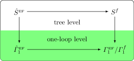
Figure 1: Transition between different formulations

The question of the equivalence between $f(R)$ gravity and its scalar-tensor formulation is related to the similar question of equivalence between different field parametrizations in scalar-tensor theories. In particular, there is a rather old but still ongoing debate about the equivalence of the so-called Jordan frame and Einstein frame parametrizations used in cosmological models Dicke (1962); Bergmann (1968); Magnano and Sokolowski (1994); Faraoni and Gunzig (1999); Nojiri and Odintsov (2001); Capozziello et al. (2010); Calmet and Yang (2013); Steinwachs and Kamenshchik (2013); Prokopec and Weenink (2013); Chiba and Yamaguchi (2013); Kamenshchik and Steinwachs (2015); Postma and Volponi (2014); Jarv et al. (2015); Domènech and Sasaki (2015); Herrero-Valea (2016); Kamenshchik et al. (2016); Pandey et al. (2016); Jarv et al. (2017); Bahamonde et al. (2017); Bhattacharya and Majhi (2017); Karam et al. (2017). The quantum equivalence between the Jordan frame and the Einstein frame has been investigated in Kamenshchik and Steinwachs (2015), by an explicit comparison of the one-loop divergences – similar to the analysis in this paper. Beside the similarity to Kamenshchik and Steinwachs (2015) in the method of comparison, the underlying problem for $f(R)$ gravity is different.

The transition between Einstein frame and Jordan frame maps a second order scalar-tensor theory of the two fields $(\hat{g}_{\mu\nu},\hat{\varphi})$ to a second order scalar-tensor theory of the two fields $(g_{\mu\nu},\varphi)$. In contrast, the transition between the Einstein frame scalar-tensor theory and $f(R)$ gravity maps a second order theory of the fields $(\hat{g}_{\mu\nu},\hat{\varphi})$ to a purely gravitational fourth order theory of one field $g_{\mu\nu}$. Therefore, the explicit transformation rules are not only non-linear but also involve derivatives.

The paper is structured as follows. In Sec. II, we present the Jordan frame and the Einstein frame formulation of scalar-tensor theories and provide the result for the one-loop divergences of the latter. In Sec. III, we discuss $f(R)$ gravity and its one-loop divergences. In Sec. IV, we derive the explicit transformation laws for the transition from the Einstein frame scalar-tensor formulation to $f(R)$ gravity. In Sec. V, we transform the one-loop divergences for the Einstein frame scalar-tensor formulation to its $f(R)$ formulation and compare the result to the one-loop divergences obtained directly for $f(R)$ gravity. In Sec. VI, we summarize our main results and discuss their implications.

II Scalar tensor theory

The Euclidean action of a scalar-tensor theory for a single scalar field $\varphi$ can be parametrized by three arbitrary functions $U(\varphi)$, $G(\varphi)$ and $V(\varphi)$,

$$S^{\text{\tiny JF}}[g,\varphi]=\int{\rm d}^{4}x\,g^{\nicefrac{{1}}{{2}}}\left(-UR+\frac{G}{2}g^{\mu\nu}\partial_{\mu}\varphi\,\partial_{\nu}\varphi+V\right)\,.$$ (1)

This representation of scalar-tensor theories is called Jordan frame (JF) parametrization. Performing a conformal transformation of the metric field $g_{\mu\nu}$ and a redefinition of the scalar field $\varphi$,

$$\tensor{\hat{g}}{{}_{\mu}{}_{\nu}}=\frac{U}{U_{0}}\tensor{g}{{}_{\mu}{}_{\nu}}\,,\;\;\left(\frac{\partial\hat{\varphi}}{\partial\varphi}\right)^{2}=\left(\frac{U_{0}}{U}\right)\frac{G\,U+3\,(U_{1})^{2}}{U}\,,$$ (2)

where $U_{1}=\partial U(\varphi)/\partial\varphi$, the action (1) transforms into

$$\hat{S}^{\text{\tiny EF}}[\hat{g},\hat{\varphi}]=\int{\rm d}^{4}x\,\hat{g}^{\nicefrac{{1}}{{2}}}\left(-U_{0}\,\hat{R}+\frac{1}{2}\hat{g}^{\mu\nu}\partial_{\mu}\hat{\varphi}\,\partial_{\nu}\hat{\varphi}+\hat{V}\right)\,.$$ (3)

The action (3) resembles the Einstein-Hilbert action for $\hat{g}_{\mu\nu}$ with a minimally coupled scalar field $\hat{\varphi}$. Consequently, the parametrization in terms of the variables $(\hat{g}_{\mu\nu},\hat{\varphi})$ is called Einstein frame (EF). Here, $U_{0}$ is a constant, usually identified with the Planck mass ${U_{0}=M_{\mathrm{P}}^{2}/2}$ and $\hat{V}$ is the EF potential, defined by

$$\hat{V}(\hat{\varphi})\coloneqq U_{0}^{2}\,\frac{V(\varphi)}{U^{2}(\varphi)}\Big{|}_{\varphi=\hat{\varphi}}\,.$$ (4)

Extremizing the EF action (3) with respect to $\hat{g}_{\mu\nu}$ and $\hat{\varphi}$ gives rise to the Einstein equation for $\hat{g}_{\mu\nu}$ and the Klein-Gordon equation for $\hat{\varphi}$,

$$\tensor{\hat{R}}{{}_{\mu}{}_{\nu}}-\frac{1}{2}\hat{R}\,\tensor{\hat{g}}{{}_{\mu}{}_{\nu}} =\frac{1}{2U_{0}}\tensor{*}{T}{{}^{\hat{\varphi}}_{\mu}{}_{\nu}}\,,\qquad\hat{\Delta}\,\hat{\varphi}=-\hat{V}_{1}\,.$$ (5)

Here, $\hat{\Delta}\coloneqq-\tensor{\hat{g}}{{}^{\mu}{}^{\nu}}\tensor{\hat{\nabla}}{{}_{\mu}}\!\tensor{\hat{\nabla}}{{}_{\nu}}$ is the Laplacian and $\tensor{*}{T}{{}^{\hat{\varphi}}_{\mu}{}_{\nu}}$ is the scalar field energy momentum tensor

$$\tensor{*}{T}{{}^{\hat{\varphi}}_{\mu}{}_{\nu}}\coloneqq{} \tensor{\partial}{{}_{\mu}}\hat{\varphi}\,\tensor{\partial}{{}_{\nu}}\hat{\varphi}-\frac{1}{2}\tensor{\hat{g}}{{}_{\mu}{}_{\nu}}\left(\tensor{\hat{g}}{{}^{\alpha}{}^{\beta}}\tensor{\partial}{{}_{\alpha}}\hat{\varphi}\,\tensor{\partial}{{}_{\beta}}\hat{\varphi}+2\hat{V}\right)\,.$$ (6)

We denote derivatives of the EF potential $\hat{V}$ with respect to the EF scalar field $\hat{\varphi}$ by

$$\hat{V}_{n}\coloneqq\frac{\partial^{n}\hat{V}}{\partial\hat{\varphi}^{n}}\,.$$ (7)

The calculation of the one-loop effective action requires a proper gauge fixing. In Barvinsky et al. (1993); Kamenshchik and Steinwachs (2015), the background covariant de Donder gauge condition is used

$$\tensor{\hat{\chi}}{{}^{\alpha}}[\hat{g},\hat{h}] =-\tensor{\hat{g}}{{}^{\alpha}{}^{\mu}}\tensor{\hat{g}}{{}^{\beta}{}^{\nu}}\left(\tensor{\hat{\nabla}}{{}_{\beta}}\tensor{\hat{h}}{{}_{\mu}{}_{\nu}}-\frac{1}{2}\tensor{\hat{\nabla}}{{}_{\mu}}\tensor{\hat{h}}{{}_{\beta}{}_{\nu}}\right)\,.$$ (8)

The covariant derivative $\hat{\nabla}_{\mu}$ is defined with respect to the metric $\hat{g}_{\mu\nu}$. The one-loop divergences for the EF action (3), obtained in Barvinsky et al. (1993); Kamenshchik and Steinwachs (2015), read

$$\hat{\varGamma}_{1}^{\text{\tiny EF}}\big{|}^{\mathrm{div}}=\frac{1}{32\,\pi^{2}\varepsilon}\int{\rm d}^{4}x\,\hat{g}^{\nicefrac{{1}}{{2}}} \Bigg{\{}-\frac{71}{60}\hat{\mathcal{G}}-\frac{43}{60}\hat{R}_{\mu\nu}\hat{R}^{\mu\nu}-\frac{1}{40}\hat{R}^{2}+\frac{1}{6}\hat{R}\hat{V}_{2}-\frac{1}{2}\left(\hat{V}_{2}\right)^{2}$$

$$+U_{0}^{-1}\left[\frac{13}{3}\hat{R}\,\hat{V}+\frac{1}{3}\hat{R}\,\left(\partial_{\mu}\hat{\varphi}\partial^{\mu}\hat{\varphi}\right)+2\,\left(\hat{V}_{1}\right)^{2}+2\,\hat{V}_{2}\left(\partial_{\mu}\hat{\varphi}\partial^{\mu}\hat{\varphi}\right)\right]$$

$$-U_{0}^{-2}\left[5\,\hat{V}^{2}+\hat{V}\left(\partial_{\mu}\hat{\varphi}\partial^{\mu}\hat{\varphi}\right)+\frac{5}{4}\left(\partial_{\mu}\hat{\varphi}\partial^{\mu}\hat{\varphi}\right)^{2}\right]\Bigg{\}}\,.$$ (9)

The Gauss-Bonnet term in the EF parametrization is defined as

$$\mathcal{\hat{G}}\coloneqq{} \tensor{\hat{R}}{{}_{\mu\nu\rho\sigma}}\tensor{\hat{R}}{{}^{\mu\nu\rho\sigma}}-4\tensor{*}{\hat{R}}{{}_{\mu\nu}}\tensor{*}{\hat{R}}{{}^{\mu\nu}}+\hat{R}^{2}\,.$$ (10)

It is understood that the indices in (9) and (10) are raised and lowered with the metric $\hat{g}_{\mu\nu}$.

III $f(R)$ gravity

The Euclidean action functional for $f(R)$ theories is given by

$$S^{f}[g]=-\int\mathop{}\!\mathrm{d}^{4}x\,g^{\nicefrac{{1}}{{2}}}\,f(R).$$ (11)

We denote derivatives of the function $f$ with respect to its argument by a subindex

$$f_{n}\coloneqq\frac{\partial^{n}\!f(R)}{\partial R^{n}}\,.$$ (12)

The extremal is defined as

$$\tensor{\mathscr{E}}{{}_{\mu}{}_{\nu}}\coloneqq{} \tensor{g}{{}_{\mu}{}_{\alpha}}\tensor{g}{{}_{\nu}{}_{\beta}}\,g^{-\nicefrac{{1}}{{2}}}\,\frac{\delta S[g]}{\delta\tensor{g}{{}_{\alpha}{}_{\beta}}}$$

$$={} -\Delta f_{1}\,\tensor{g}{{}_{\mu}{}_{\nu}}-\nabla_{\mu}\nabla_{\nu}f_{1}+f_{1}\tensor{*}{R}{{}_{\mu}{}_{\nu}}-\frac{1}{2}f\tensor{g}{{}_{\mu}{}_{\nu}}\,.$$ (13)

The classical equations of motion are satisfied, if $\tensor{\mathscr{E}}{{}_{\mu}{}_{\nu}}=0$. The trace of the extremal reads

$$\mathscr{E}\coloneqq\tensor{g}{{}^{\mu}{}^{\nu}}\mathscr{E}_{\mu\nu}=-3\,\Delta f_{1}+Rf_{1}-2f\,.$$ (14)

We also define the rescaled extremal and its trace

$$\tensor{E}{{}_{\mu}{}_{\nu}}\coloneqq\frac{\tensor{\mathscr{E}}{{}_{\mu}{}_{\nu}}}{(-f_{1})},\qquad E\coloneqq\tensor{g}{{}^{\mu}{}^{\nu}}E_{\mu\nu}=\frac{\mathscr{E}}{(-f_{1})}\,.$$ (15)

Both, $E_{\mu\nu}$ and $E$, are homogeneous functions of degree zero in $f$ and its derivatives $f_{n}$. The one-loop divergences for $f(R)$ gravity have been calculated recently Ruf and Steinwachs (2017) in the extended de Donder gauge

$$\tensor{\chi}{{}^{\alpha}}[g,h] =-\tensor{g}{{}^{\alpha}{}^{\mu}}\tensor{g}{{}^{\beta}{}^{\nu}}\left(\tensor{\nabla}{{}_{\beta}}\tensor{h}{{}_{\mu}{}_{\nu}}-\frac{1}{2}\tensor{\nabla}{{}_{\mu}}\tensor{h}{{}_{\beta}{}_{\nu}}+\tensor{\Upsilon}{{}_{\beta}}\tensor{h}{{}_{\mu}{}_{\nu}}\right)\,.$$ (16)

The additional term is linear in

$$\tensor{\Upsilon}{{}_{\mu}}\coloneqq\partial_{\mu}\ln f_{1}=\frac{f_{2}}{f_{1}}\partial_{\mu}R\,.$$ (17)

The divergent part of the one-loop effective action for $f(R)$ gravity on an arbitrary background reads Ruf and Steinwachs (2017)

$$\varGamma_{1}^{f}\big{|}^{\mathrm{div}}={} \frac{1}{32\pi^{2}\varepsilon}\int{\rm d}^{4}x\,g^{\nicefrac{{1}}{{2}}}\left[-\frac{71}{60}\mathcal{G}-\frac{609}{80}\tensor{*}{R}{{}_{\mu}{}_{\nu}}R^{\mu\nu}+\frac{1}{3}\frac{f}{f_{2}}-\frac{115}{288}\left(\frac{f}{f_{1}}\right)^{2}-\frac{1}{18}\left(\frac{f_{1}}{f_{2}}\right)^{2}\right.$$

$$\left.-\frac{15}{64}\frac{f}{f_{1}}\,R+\frac{3919}{1440}R^{2}+\frac{15}{64}R\,\Delta\ln f_{1}+E\left(\frac{55}{108}E-\frac{419}{432}\frac{f}{f_{1}}+\frac{2933}{864}R+\frac{221}{288}\Delta\ln f_{1}\right)\right.$$

$$\left.-\tensor{E}{{}_{\mu}{}_{\nu}}\left(\frac{403}{96}\tensor{E}{{}^{\mu}{}^{\nu}}+\frac{2987}{288}\tensor{*}{R}{{}^{\mu}{}^{\nu}}\right)\right]\,,$$ (18)

with the Gauss-Bonnet term

$$\mathcal{G}\coloneqq{} \tensor{R}{{}_{\mu\nu\rho\sigma}}\tensor{R}{{}^{\mu\nu\rho\sigma}}-4\tensor{*}{R}{{}_{\mu\nu}}\tensor{*}{R}{{}^{\mu\nu}}+R^{2}\,.$$ (19)

IV Transition between $f(R)$ theories and scalar-tensor theories in the Einstein frame

The action (11) for $f(R)$ gravity admits a scalar-tensor formulation, where the extra scalar degree of freedom, included in the higher derivative structure of $f(R)$ gravity, becomes manifest. The transformation can be performed in two steps. First we introduce an auxiliary scalar field $\chi$, perform a Legendre transformation and represent the action for $f(R)$ gravity as a scalar-tensor theory (1) in the JF formulation for the JF scalar field $\varphi$. In a second step, we perform the transformation (2) to the EF formulation (3). In this way, all information about the original function $f(R)$ is encoded in the EF potential (4) and the EF field $\hat{\varphi}$.

Starting from the action (11), we introduce the auxiliary scalar field $\chi$ and perform a Legendre transformation

$$S_{\mathrm{aux}}[g,\chi]=-\int{\rm d}^{4}x\,g^{\nicefrac{{1}}{{2}}}\left[f(\chi)+f_{1}(\chi)(R-\chi)\right]\,.$$ (20)

Extremizing (20) with respect to $\chi$ leads to the equation

$$f_{2}\left(R-\chi\right)=0\,.$$ (21)

For $f_{2}\neq 0$ this implies

$$\chi=R\,.$$ (22)

Therefore, “on-shell” the action (20) is equivalent to the original action (11). We define the scalar function $U(\varphi)$

$$U(\varphi)\coloneqq f_{1}(\chi)\,.$$ (23)

Given a function $f(\chi)$, this relation has to be inverted and explicitly solved for $\chi(\varphi)=\chi(U(\varphi))$. In terms of (23), the action (20) acquires the form of a scalar-tensor theory (1) with $G(\varphi)=0$,

$$S_{\mathrm{aux}}[g,\varphi]=\int{\rm d}^{4}x\,g^{\nicefrac{{1}}{{2}}}\left[-U(\varphi)R+V(\varphi)\right]\,.$$ (24)

The JF potential is given by

$$V(\varphi)\coloneqq U(\varphi)\chi(\varphi)-f(\chi(\varphi))\,.$$ (25)

Using (2) with $G=0$, we obtain the EF scalar-tensor formulation (3) for $f(R)$ gravity.

In order to compare the different formulations, we provide the explicit transformations that bring the EF scalar-tensor theory back to its corresponding $f(R)$ formulation. First, we present the transformations for the scalar field and its derivatives as well as for the scalar field potential and its derivatives. The special property $G=0$ of $f(R)$ theories allows to immediately integrate the differential relation (2). Using (23), we express the EF field $\hat{\varphi}$ in terms of the scalar curvature $R$,

$$\hat{\varphi}(R)=(3\,U_{0})^{\nicefrac{{1}}{{2}}}\ln\,f_{1}(R)\,.$$ (26)

This implies the relation

$$\frac{\partial R}{\partial\hat{\varphi}}=(3\,U_{0})^{-\nicefrac{{1}}{{2}}}\frac{f_{1}}{f_{2}}\,.$$ (27)

Combining (26) with (17), we obtain

$$\partial_{\mu}\hat{\varphi}=(3\,U_{0})^{\nicefrac{{1}}{{2}}}\,\tensor{\Upsilon}{{}_{\mu}}\,.$$ (28)

Using (4), (22) and (23), the EF potential can be expressed as a function of scalar curvature $R$,

$$\hat{V}(R)=U_{0}^{2}\,\frac{R\,f_{1}-f}{f_{1}^{2}}\,.$$ (29)

With (27), we find for the first and second derivatives

$$\hat{V}_{1}(R)={} U_{0}^{2}\,(3\,U_{0})^{-\nicefrac{{1}}{{2}}}\left[\frac{2\,f-R\,f_{1}}{\left(f_{1}\right)^{2}}\right],$$ (30)

$$\hat{V}_{2}(R)={} \frac{U_{0}}{3f_{2}}\left[\frac{\left(f_{1}\right)^{2}+R\,f_{1}\,f_{2}-4f\,f_{2}}{\left(f_{1}\right)^{2}}\right].$$ (31)

Second, we collect the conformal transformation rules. Combing (2) with (22) and (23), we find

$$\tensor{\hat{g}}{{}_{\mu}{}_{\nu}}={} \frac{f_{1}}{U_{0}}\tensor{g}{{}_{\mu}{}_{\nu}}\,,$$ (32)

$$\tensor{\hat{g}}{{}^{\mu}{}^{\nu}}={} \frac{U_{0}}{f_{1}}\tensor{g}{{}^{\mu}{}^{\nu}}\,,$$ (33)

$$\hat{g}^{\nicefrac{{1}}{{2}}}={} \left(\frac{f_{1}}{U_{0}}\right)^{2}g^{\nicefrac{{1}}{{2}}}\,,$$ (34)

$$\tensor{\hat{\Gamma}}{{}^{\lambda}_{\mu\nu}}={} \tensor{\Gamma}{{}^{\lambda}_{\mu\nu}}+\tensor{*}{\delta}{{}^{\lambda}_{(\mu}}\tensor{\Upsilon}{{}_{\nu)}}-\frac{1}{2}\tensor{g}{{}_{\mu\nu}}\tensor{\Upsilon}{{}^{\lambda}}\,,$$ (35)

$$\tensor{\hat{R}}{{}^{\lambda}_{\mu}{}_{\nu}{}_{\rho}}={} \tensor{R}{{}^{\lambda}_{\mu}{}_{\nu}{}_{\rho}}-\frac{1}{2}\tensor{*}{\delta}{{}^{\lambda}_{[\nu}}\tensor{g}{{}_{\rho]}{}_{\mu}}\tensor{g}{{}^{\alpha}{}^{\beta}}\tensor{\Upsilon}{{}_{\alpha}}\tensor{\Upsilon}{{}_{\beta}}$$

$$+\frac{1}{2}\left(\tensor{*}{\delta}{{}^{\lambda}_{[\nu}}\tensor{\Upsilon}{{}_{\rho]}}\tensor{\Upsilon}{{}_{\mu}}-\tensor{g}{{}^{\lambda}{}^{\alpha}}\tensor{g}{{}_{\mu}{}_{[\nu}}\tensor{\Upsilon}{{}_{\rho]}}\tensor{\Upsilon}{{}_{\alpha}}\right)$$

$$-\left(\tensor{*}{\delta}{{}^{\lambda}_{[\nu}}\tensor{\nabla}{{}_{\rho]}}\tensor{\Upsilon}{{}_{\mu}}-\tensor{g}{{}^{\lambda}{}^{\alpha}}\tensor{g}{{}_{\mu}{}_{[\nu}}\tensor{\nabla}{{}_{\rho]}}\tensor{\Upsilon}{{}_{\alpha}}\right)\,,$$ (36)

$$\tensor{\hat{R}}{{}_{\mu}{}_{\nu}}={} \tensor{*}{R}{{}_{\mu}{}_{\nu}}-\frac{1}{2}\tensor{g}{{}_{\mu}{}_{\nu}}\tensor{g}{{}^{\alpha}{}^{\beta}}\left(\tensor{\Upsilon}{{}_{\alpha}}\tensor{\Upsilon}{{}_{\beta}}+\tensor{\nabla}{{}_{\alpha}}\tensor{\Upsilon}{{}_{\beta}}\right)$$

$$+\frac{1}{2}\tensor{\Upsilon}{{}_{\mu}}\tensor{\Upsilon}{{}_{\nu}}-\tensor{\nabla}{{}_{\mu}}\tensor{\Upsilon}{{}_{\nu}}\,,$$ (37)

$$\hat{R}={} \frac{U_{0}}{f_{1}}\left[R-\frac{3}{2}\tensor{g}{{}^{\alpha}{}^{\beta}}\left(\tensor{\Upsilon}{{}_{\alpha}}\tensor{\Upsilon}{{}_{\beta}}+2\tensor{\nabla}{{}_{\alpha}}\tensor{\Upsilon}{{}_{\beta}}\right)\right]\,,$$ (38)

In particular, combining (28) with (33) and (35), the Laplacian of the EF scalar field transforms as

$$\hat{\Delta}\hat{\varphi}={} (3\,U_{0})^{\nicefrac{{1}}{{2}}}\frac{U_{0}}{f_{1}^{2}}\Delta f_{1}\,.$$ (39)

V Comparison

Using the explicit transition formulas, provided in the last section, we transform all quantities in the EF formulation to the corresponding expressions in the $f(R)$ formulation and compare them at the classical and quantum level. For the explicit transformations (26) – (39) not to be singular, we require $f_{1}\neq 0$. Moreover, for (23) to be invertible, we require $f_{2}\neq 0$.

V.1 Tree-level comparison

By construction, the action of the scalar-tensor theory (3) in the EF parametrization is equivalent to the action of $f(R)$ gravity (11), which can be easily verified by applying the transformation laws (26) – (39) to (3).

Likewise, the Einstein equation is easily seen to be equivalent to the equation of motion $E_{\mu\nu}=0$ for $f(R)$ gravity by applying (26) – (39) to (5). In addition, the Klein-Gordon equation for the scalar field in (5) transforms into the trace of the on-shell condition $E=0$, which therefore does not encode any new information. In particular, the equivalence of the equations of motion for scalar-tensor theories and $f(R)$ gravity implies that the on-shell condition can be imposed in either formulation.

V.2 One-loop comparison

We apply the transformation formulas (26) – (39) to the divergent part of the off-shell one-loop effective action $\hat{\varGamma}_{1}^{\text{\tiny EF}}$, calculated in the EF (9). In this way, we express $\hat{\varGamma}_{1}^{\text{\tiny EF}}$ in terms of its $f(R)$ formulation $\varGamma_{1}^{\text{\tiny EF}}$. Subsequent use of the integration by parts identities, provided in Appendix A, allows to write $\varGamma_{1}^{\text{\tiny EF}}$ in terms of the rescaled extremal $E_{\mu\nu}$,

$$\left.\varGamma_{1}^{\text{\tiny EF}}\right|^{\mathrm{div}} =\frac{1}{32\pi^{2}\varepsilon}\int{\rm d}^{4}x\,g^{\nicefrac{{1}}{{2}}}\left[-\frac{71}{60}\mathcal{G}-\frac{609}{80}\tensor{*}{R}{{}_{\mu}{}_{\nu}}R^{\mu\nu}+\frac{1}{3}\frac{f}{f_{2}}-\frac{115}{288}\left(\frac{f}{f_{1}}\right)^{2}-\frac{1}{18}\left(\frac{f_{1}}{f_{2}}\right)^{2}\right.$$

$$\left.-\frac{15}{64}\frac{f}{f_{1}}\,R+\frac{3919}{1440}R^{2}+\frac{15}{64}R\,\Delta\ln f_{1}+E\left(-\frac{1}{3}E+\frac{47}{48}\frac{f}{f_{1}}+\frac{1}{18}\frac{f_{1}}{f_{2}}+\frac{695}{288}R+\frac{117}{32}\Delta\ln f_{1}\right)\right.$$

$$\left.-\tensor{E}{{}_{\mu}{}_{\nu}}\left(\frac{331}{96}\tensor{E}{{}^{\mu}{}^{\nu}}+\frac{331}{32}\tensor{*}{R}{{}^{\mu}{}^{\nu}}\right)\right]\,.$$ (40)

Note that there is one additional structure in (40), proportional to $E\,f_{1}/f_{2}$, which is not present in (18). Comparing (40) to the off-shell one-loop divergences (18), obtained directly for $f(R)$ gravity, we find that the two off-shell results do not coincide. The difference is given by

$$\varGamma_{1}^{f}\big{|}^{\mathrm{div}}-\varGamma_{1}^{\text{\tiny EF}}\big{|}^{\mathrm{div}}$$

$$={} \frac{1}{32\pi^{2}\varepsilon}\int{\rm d}^{4}x\,g^{\nicefrac{{1}}{{2}}}E_{\mu\nu}\left[-\frac{3}{4}\tensor{E}{{}^{\mu}{}^{\nu}}-\frac{1}{36}\tensor{*}{R}{{}^{\mu}{}^{\nu}}+\left(\frac{91}{108}E\right.\right.$$

$$\left.\left.+\frac{53}{54}R-\frac{421}{216}\frac{f}{f_{1}}-\frac{1}{18}\frac{f_{1}}{f_{2}}-\frac{26}{9}\Delta\ln f_{1}\right)g^{\mu\nu}\right].$$ (41)

Independent of the choice for the scalar function $f$, the difference between the off-shell divergences never vanishes due to terms proportional to $\tensor{R}{{}_{\mu\nu}}\tensor{R}{{}^{\mu\nu}}$ in the first line of (41). It is clear that the non-equivalence is a pure off-shell effect, as the difference (41) vanishes on-shell $E_{\mu\nu}=0$. Therefore, on-shell, the one-loop divergences for $f(R)$ gravity and its scalar-tensor formulation in the EF are equivalent at the quantum level.

VI Conclusion

We have investigated the quantum equivalence of $f(R)$ theories and scalar-tensor theories by explicitly comparing the one-loop divergences in both formulations for arbitrary background fields. We find that the off-shell one-loop divergences are ambiguous, as they depend on the formulation, while their on-shell reduction is not. Our on-shell agreement also provides a strong independent check of the on-shell structures in the result for the one-loop divergences of $f(R)$ gravity obtained in Ruf and Steinwachs (2017).

On-shell equivalence of $f(R)$ gravity and scalar-tensor theories has also been found in Bamba et al. (2014) for certain cosmological models on a de Sitter background. The equivalence of $f(R)$ gravity and Brans-Dicke theory has been studied previously in the context of the exact renormalization group Benedetti and Guarnieri (2014). Although we do not fully agree with their interpretation of the result, their conclusion also seems to support the statement that the off-shell divergences depend on the formulation. A similar result has been obtained in Kamenshchik and Steinwachs (2015), where the quantum equivalence of scalar-tensor theories in the JF and EF formulation has been analyzed. There, it has been found that the off-shell divergences are parametrization dependent while on-shell the equivalence is retained. This on-shell equivalence is to be expected on the grounds of formal equivalence theorems Chisholm (1961); Kamefuchi et al. (1961); Coleman et al. (1969); Kallosh and Tyutin (1973); Tyutin (1982).

The off-shell non-equivalence is not a physical effect but a defect of the underlying mathematical formalism. The significance of this problem in cosmology might be best explained in the context of inflationary models. In general, off-shell UV divergences lead to running couplings, whose Renormalization Group (RG) flow is controlled by the corresponding beta functions. Any ambiguity in the off-shell divergences will therefore induce a corresponding ambiguity in the beta functions and consequently an ambiguity in the values of the coupling constants. The ambiguity of the beta functions and the couplings is not yet a real problem because neither of them are physical observables. The problem in inflationary cosmology arises when these running couplings are evaluated at the energy scale of inflation and simply inserted into the cosmological parameters. These parameters, which inherit the ambiguity from the coupling constants, are then compared to observational data. But what meaning does such a procedure really have?

In order to obtain reliable predictions, it seems to be of crucial importance to define unambiguous cosmological quantum observables, which are in particular manifestly gauge and parametrization independent.

Appendix A Integration by parts identities

We can express the $\tensor{\Upsilon}{{}_{\mu}}$-dependent invariants in terms of $\tensor{E}{{}_{\mu}{}_{\nu}}$ and its trace $E$ by the following set of identities derived in Ruf and Steinwachs (2017),

$$\tensor{\Upsilon}{{}^{\mu;\nu}}={} \tensor{E}{{}^{\mu}{}^{\nu}}-\frac{1}{3}\left(E+R-\frac{1}{2}\frac{f}{f_{1}}\right)\tensor{g}{{}^{\mu}{}^{\nu}}$$

$$+\tensor{*}{R}{{}^{\mu}{}^{\nu}}-\tensor{\Upsilon}{{}^{\mu}}\tensor{\Upsilon}{{}^{\nu}}\,,$$ (42)

$$(\tensor{\Upsilon}{{}_{\mu}}\tensor{\Upsilon}{{}^{\mu}})^{2}\overset{\bullet}{=}{} -\frac{1}{3}\left(E+R-\frac{f}{f_{1}}\right)(\tensor{\Upsilon}{{}_{\mu}}\tensor{\Upsilon}{{}^{\mu}})$$

$$+\frac{2}{3}\left(\tensor{E}{{}_{\mu}{}_{\nu}}+\tensor{*}{R}{{}_{\mu}{}_{\nu}}\right)\tensor{\Upsilon}{{}^{\mu}}\tensor{\Upsilon}{{}^{\nu}}\,,$$ (43)

$$\frac{f_{1}}{f_{2}}(\tensor{\Upsilon}{{}_{\mu}}\tensor{\Upsilon}{{}^{\mu}})\overset{\bullet}{=}{} R\,\Delta\ln f_{1}\,,$$ (44)

$$\frac{f}{f_{1}}(\tensor{\Upsilon}{{}_{\mu}}\tensor{\Upsilon}{{}^{\mu}})\overset{\bullet}{=}{} -\frac{1}{6}\left(E+R-2\frac{f}{f_{1}}\right)\frac{f}{f_{1}}$$

$$+\frac{1}{2}R\,\Delta\ln f_{1}\,,$$ (45)

$$R\,(\tensor{\Upsilon}{{}_{\mu}}\tensor{\Upsilon}{{}^{\mu}})\overset{\bullet}{=}{} -\frac{1}{3}\left(E+R-2\frac{f}{f_{1}}\right)R$$

$$+R\,\Delta\ln f_{1}\,,$$ (46)

$$E\,(\tensor{\Upsilon}{{}_{\mu}}\tensor{\Upsilon}{{}^{\mu}})\overset{\bullet}{=}{} -\frac{1}{3}\left(E+R-2\frac{f}{f_{1}}\right)E$$

$$+E\,\Delta\ln f_{1}\,,$$ (47)

$$\tensor{E}{{}_{\mu}{}_{\nu}}\tensor{\Upsilon}{{}^{\mu}}\tensor{\Upsilon}{{}^{\nu}}\overset{\bullet}{=}{} \frac{1}{2}\tensor{E}{{}_{\mu}{}_{\nu}}\tensor{E}{{}^{\mu}{}^{\nu}}+\frac{1}{2}\tensor{E}{{}_{\mu}{}_{\nu}}\tensor{*}{R}{{}^{\mu}{}^{\nu}}$$

$$-\frac{1}{6}E\left(E+R-\frac{1}{2}\frac{f}{f_{1}}\right)\,,$$ (48)

$$\tensor{*}{R}{{}_{\mu}{}_{\nu}}\tensor{\Upsilon}{{}^{\mu}}\tensor{\Upsilon}{{}^{\nu}}\overset{\bullet}{=}{} \tensor{E}{{}_{\mu}{}_{\nu}}\tensor{*}{R}{{}^{\mu}{}^{\nu}}+\tensor{*}{R}{{}_{\mu}{}_{\nu}}\tensor{*}{R}{{}^{\mu}{}^{\nu}}$$

$$-\frac{R}{3}\left(E+R-\frac{1}{2}\frac{f}{f_{1}}\right)$$

$$+\frac{1}{2}R\,\Delta\ln f_{1}\,.$$ (49)

References

- Sotiriou and Faraoni (2010) T. P. Sotiriou and V. Faraoni, Rev. Mod. Phys. 82, 451 (2010), arXiv:0805.1726 [gr-qc] .
- De Felice and Tsujikawa (2010) A. De Felice and S. Tsujikawa, Living Rev. Rel. 13, 3 (2010), arXiv:1002.4928 [gr-qc] .
- Nojiri and Odintsov (2011) S. Nojiri and S. D. Odintsov, Phys. Rept. 505, 59 (2011), arXiv:1011.0544 [gr-qc] .
- Clifton et al. (2012) T. Clifton, P. G. Ferreira, A. Padilla, and C. Skordis, Phys. Rept. 513, 1 (2012), arXiv:1106.2476 [astro-ph.CO] .
- Nojiri et al. (2017) S. Nojiri, S. D. Odintsov, and V. K. Oikonomou, Phys. Rept. 692, 1 (2017), arXiv:1705.11098 [gr-qc] .
- Stelle (1977) K. S. Stelle, Phys. Rev. D16, 953 (1977).
- Stelle (1978) K. S. Stelle, Gen. Rel. Grav. 9, 353 (1978).
- Starobinsky (1980) A. A. Starobinsky, Phys. Lett. 91B, 99 (1980).
- Woodard (2007) R. P. Woodard, The invisible universe: Dark matter and dark energy. Proceedings, 3rd Aegean School, Karfas, Greece, September 26-October 1, 2005, Lect. Notes Phys. 720, 403 (2007), arXiv:astro-ph/0601672 [astro-ph] .
- Bezrukov and Shaposhnikov (2008) F. L. Bezrukov and M. Shaposhnikov, Phys. Lett. B659, 703 (2008), arXiv:0710.3755 [hep-th] .
- Barvinsky et al. (2008) A. O. Barvinsky, A. Yu. Kamenshchik, and A. A. Starobinsky, JCAP 11, 021 (2008), arXiv:0809.2104 [hep-ph] .
- Bezrukov et al. (2009) F. L. Bezrukov, A. Magnin, and M. Shaposhnikov, Phys. Lett. B675, 88 (2009), arXiv:0812.4950 [hep-ph] .
- De Simone et al. (2009) A. De Simone, M. P. Hertzberg, and F. Wilczek, Phys. Lett. B678, 1 (2009), arXiv:0812.4946 [hep-ph] .
- Barvinsky et al. (2009) A. O. Barvinsky, A. Yu. Kamenshchik, C. Kiefer, A. A. Starobinsky, and C. Steinwachs, JCAP 0912, 003 (2009), arXiv:0904.1698 [hep-ph] .
- Bezrukov and Shaposhnikov (2009) F. Bezrukov and M. Shaposhnikov, JHEP 07, 089 (2009), arXiv:0904.1537 [hep-ph] .
- Barvinsky et al. (2012) A. O. Barvinsky, A. Yu. Kamenshchik, C. Kiefer, A. A. Starobinsky, and C. F. Steinwachs, Eur. Phys. J. C72, 2219 (2012), arXiv:0910.1041 [hep-ph] .
- Bezrukov et al. (2011) F. Bezrukov, A. Magnin, M. Shaposhnikov, and S. Sibiryakov, JHEP 01, 016 (2011), arXiv:1008.5157 [hep-ph] .
- Bezrukov and Gorbunov (2012) F. L. Bezrukov and D. S. Gorbunov, Phys. Lett. B713, 365 (2012), arXiv:1111.4397 [hep-ph] .
- Kehagias et al. (2014) A. Kehagias, A. Moradinezhad Dizgah, and A. Riotto, Phys. Rev. D89, 043527 (2014), arXiv:1312.1155 [hep-th] .
- Ruf and Steinwachs (2017) M. S. Ruf and C. F. Steinwachs, (2017), arXiv:1711.04785 [gr-qc] .
- Barvinsky et al. (1993) A. O. Barvinsky, A. Yu. Kamenshchik, and I. P. Karmazin, Phys. Rev. D48, 3677 (1993), arXiv:gr-qc/9302007 [gr-qc] .
- Kamenshchik and Steinwachs (2015) A. Yu. Kamenshchik and C. F. Steinwachs, Phys. Rev. D91, 084033 (2015), arXiv:1408.5769 [gr-qc] .
- Dicke (1962) R. H. Dicke, Phys. Rev. 125, 2163 (1962).
- Bergmann (1968) P. G. Bergmann, Int. J. Theor. Phys. 1, 25 (1968).
- Magnano and Sokolowski (1994) G. Magnano and L. M. Sokolowski, Phys. Rev. D50, 5039 (1994), arXiv:gr-qc/9312008 [gr-qc] .
- Faraoni and Gunzig (1999) V. Faraoni and E. Gunzig, Int. J. Theor. Phys. 38, 217 (1999), arXiv:astro-ph/9910176 [astro-ph] .
- Nojiri and Odintsov (2001) S. Nojiri and S. D. Odintsov, Int. J. Mod. Phys. A16, 1015 (2001), arXiv:hep-th/0009202 [hep-th] .
- Capozziello et al. (2010) S. Capozziello, P. Martin-Moruno, and C. Rubano, Phys. Lett. B689, 117 (2010), arXiv:1003.5394 [gr-qc] .
- Calmet and Yang (2013) X. Calmet and T.-C. Yang, Int. J. Mod. Phys. A28, 1350042 (2013), arXiv:1211.4217 [gr-qc] .
- Steinwachs and Kamenshchik (2013) C. F. Steinwachs and A. Yu. Kamenshchik, Proceedings, Multiverse and Fundamental Cosmology (Multicosmofun’12): Szczecin, Poland, September 10-14, 2012, (2013), 10.1063/1.4791748, [AIP Conf. Proc.1514,161(2012)], arXiv:1301.5543 [gr-qc] .
- Prokopec and Weenink (2013) T. Prokopec and J. Weenink, JCAP 1309, 027 (2013), arXiv:1304.6737 [gr-qc] .
- Chiba and Yamaguchi (2013) T. Chiba and M. Yamaguchi, JCAP 1310, 040 (2013), arXiv:1308.1142 [gr-qc] .
- Postma and Volponi (2014) M. Postma and M. Volponi, Phys. Rev. D90, 103516 (2014), arXiv:1407.6874 [astro-ph.CO] .
- Jarv et al. (2015) L. Jarv, P. Kuusk, M. Saal, and O. Vilson, Phys. Rev. D91, 024041 (2015), arXiv:1411.1947 [gr-qc] .
- Domènech and Sasaki (2015) G. Domènech and M. Sasaki, JCAP 1504, 022 (2015), arXiv:1501.07699 [gr-qc] .
- Herrero-Valea (2016) M. Herrero-Valea, Phys. Rev. D93, 105038 (2016), arXiv:1602.06962 [hep-th] .
- Kamenshchik et al. (2016) A. Yu. Kamenshchik, E. O. Pozdeeva, S. Yu. Vernov, A. Tronconi, and G. Venturi, Phys. Rev. D94, 063510 (2016), arXiv:1602.07192 [gr-qc] .
- Pandey et al. (2016) S. Pandey, S. Pal, and N. Banerjee, (2016), arXiv:1611.07043 [gr-qc] .
- Jarv et al. (2017) L. Jarv, K. Kannike, L. Marzola, A. Racioppi, M. Raidal, M. Runkla, M. Saal, and H. Veermae, Phys. Rev. Lett. 118, 151302 (2017), arXiv:1612.06863 [hep-ph] .
- Bahamonde et al. (2017) S. Bahamonde, S. D. Odintsov, V. K. Oikonomou, and P. V. Tretyakov, Phys. Lett. B766, 225 (2017), arXiv:1701.02381 [gr-qc] .
- Bhattacharya and Majhi (2017) K. Bhattacharya and B. R. Majhi, Phys. Rev. D95, 064026 (2017), arXiv:1702.07166 [gr-qc] .
- Karam et al. (2017) A. Karam, T. Pappas, and K. Tamvakis, Phys. Rev. D96, 064036 (2017), arXiv:1707.00984 [gr-qc] .
- Shapiro and Takata (1995) I. L. Shapiro and H. Takata, Phys. Rev. D52, 2162 (1995), arXiv:hep-th/9502111 [hep-th] .
- Steinwachs and Kamenshchik (2011) C. F. Steinwachs and A. Yu. Kamenshchik, Phys. Rev. D84, 024026 (2011), arXiv:1101.5047 [gr-qc] .
- Narain and Percacci (2010) G. Narain and R. Percacci, Class. Quant. Grav. 27, 075001 (2010), arXiv:0911.0386 [hep-th] .
- Percacci and Vacca (2015) R. Percacci and G. P. Vacca, Eur. Phys. J. C75, 188 (2015), arXiv:1501.00888 [hep-th] .
- Chakraborty and SenGupta (2016) S. Chakraborty and S. SenGupta, Eur. Phys. J. C76, 552 (2016), arXiv:1604.05301 [gr-qc] .
- (48) Martín-García, José M., “xAct: Efficient tensor computer algebra for the Wolfram Language,” http://www.xact.es, Accessed: 2017-11-17.
- Brizuela et al. (2009) D. Brizuela, J. M. Martin-Garcia, and G. A. Mena Marugan, Gen. Rel. Grav. 41, 2415 (2009), arXiv:0807.0824 [gr-qc] .
- Nutma (2014) T. Nutma, Comput. Phys. Commun. 185, 1719 (2014), arXiv:1308.3493 [cs.SC] .
- Bamba et al. (2014) K. Bamba, G. Cognola, S. D. Odintsov, and S. Zerbini, Phys. Rev. D90, 023525 (2014), arXiv:1404.4311 [gr-qc] .
- Benedetti and Guarnieri (2014) D. Benedetti and F. Guarnieri, New J. Phys. 16, 053051 (2014), arXiv:1311.1081 [hep-th] .
- Chisholm (1961) J. S. R. Chisholm, Nucl. Phys. 26, 469 (1961).
- Kamefuchi et al. (1961) S. Kamefuchi, L. O’Raifeartaigh, and A. Salam, Nucl. Phys. 28, 529 (1961).
- Coleman et al. (1969) S. R. Coleman, J. Wess, and B. Zumino, Phys. Rev. 177, 2239 (1969).
- Kallosh and Tyutin (1973) R. E. Kallosh and I. V. Tyutin, Yad. Fiz. 17, 190 (1973), [Sov. J. Nucl. Phys.17,98(1973)].
- Tyutin (1982) I. V. Tyutin, Yad. Fiz. 35, 222 (1982).
- Moss (2014) I. G. Moss, (2014), arXiv:1409.2108 [hep-th] .
- Bounakis and Moss (2017) M. Bounakis and I. G. Moss, (2017), arXiv:1710.02987 [hep-th] .