Extinction and Survival in Two-Species Annihilation

Abstract

We study diffusion-controlled two-species annihilation with a finite number of particles. In this stochastic process, particles move diffusively, and when two particles of opposite type come into contact, the two annihilate. We focus on the behavior in three spatial dimensions and for initial conditions where particles are confined to a compact domain. Generally, one species outnumbers the other, and we find that the difference between the number of majority and minority species, which is a conserved quantity, controls the behavior. When the number difference exceeds a critical value, the minority becomes extinct and a finite number of majority particles survive, while below this critical difference, a finite number of particles of both species survive. The critical difference $\Delta_{c}$ grows algebraically with the total initial number of particles $N$, and when $N\gg 1$, the critical difference scales as $\Delta_{c}\sim N^{1/3}$. Furthermore, when the initial concentrations of the two species are equal, the average number of surviving majority and minority particles, $M_{+}$ and $M_{-}$, exhibit two distinct scaling behaviors, $M_{+}\sim N^{1/2}$ and $M_{-}\sim N^{1/6}$. In contrast, when the initial populations are equal, these two quantities are comparable $M_{+}\sim M_{-}\sim N^{1/3}$.

I Introduction

Theoretical studies of non-equilibrium dynamics are primarily concerned with the behavior of infinitely extended systems krb ; ut . Indeed, the statistical physics of time-dependent phenomena such as ordering krb ; ut ; ajb , avalanches dd ; sdm ; pld and reaction processes otb ; bh ; thv typically focus on scaling laws for unbounded systems composed of infinitely many interacting particles (or spins). In most cases, theoretical techniques which successfully describe infinite systems, cannot be specialized to finite ones kpwh ; fds . Yet, experimental ak ; dbm ; se and computational nb studies necessarily involve finite systems.

Reaction-diffusion processes (see krb ; otb ; bh ; thv for a review) constitute an important class of non-equilibrium dynamics cg . Recent studies show that these processes exhibit phenomena that are unique to finite systems bk ; bk1 . In particular, for reaction-controlled single-species annihilation, it was recently found that a finite number of particles may survive indefinitely. Specifically, starting with a finite number of particles which are confined to a bounded domain, a small subset of particles may “escape” far outside the initially occupied region and thereby avert annihilation. Here, we study two-species annihilation and find another phenomena, a transition from survival to extinction, together with scaling laws that are unique to finite systems.

We investigate a random process where two distinct species diffuse in unbounded space and additionally, the two species annihilate each other. While we also present results for general spatial dimensions, we focus primarily on the most interesting case of three dimensions. When a finite number of particles is initially localized within a compact domain, there are two greatly different outcomes. In the first scenario, a finite number of particles of each species survives the annihilation process. In the second scenario, one species vanishes and one species partially survives. The initial population difference controls this transition from survival to extinction.

Generally, one species outnumbers the other. Moreover, the difference between the number of majority particles and the number of minority particles is conserved throughout the annihilation process. This population difference controls the outcome of the reaction process and moreover, there is a critical difference $\Delta_{c}$. When the number difference exceeds the critical difference, all minority particles eventually vanish, but in the complementary regime, some minority particles do survive.

A number of finite-size scaling laws characterize these behaviors. First, the critical difference grows algebraically with the total number of particles $N$,

$$\Delta_{c}\sim N^{1/3}\,.$$ (1)

We investigate the total number of surviving particles from each species, and we consider two initial conditions: (i) equal populations of the two species, and (ii) equal concentrations of the two species. For equal populations, the behavior is very similar to that found for single-species annihilation bk . In this case, the average number of surviving particles $M$ grows algebraically with system size,

$$M\sim N^{1/3}\,.$$ (2)

For equal concentrations, the average number of surviving majority particles, $M_{+}$, is much larger than the average number of surviving minority particles, $M_{-}$. Interestingly, these two averages exhibit different scaling laws,

$$M_{+}\sim N^{1/2},\qquad M_{-}\sim N^{1/6}\,.$$ (3)

Neither one of these two scaling behaviors coincides with Eq. (2). Our theoretical analysis combines the rate equation approach with scaling estimates for the finite duration of the reaction process. Results of extensive numerical simulations confirm the theoretical predictions.

II Two-Species Annihilation

In the two-species annihilation process, particles are initially distributed randomly in space with a uniform concentration. There are two types of particles, denoted by $A$ and $B$. Each particle moves diffusively, the diffusion coefficient $D$ is assumed to be the same for both species. Particles of the same type do not interact but two particles of the opposite type annihilate upon contact, as represented by the reaction scheme

$$A+B\to\emptyset\,.$$ (4)

This stochastic process can be realized in continuous or discrete space. Our numerical simulations implement the discrete version where particles occupy sites of a regular lattice. Each particle performs a random walk as it moves from one lattice site to a randomly-chosen neighboring site. Annihilation occurs whenever a particle lands on a site that is occupied by a particle of the opposite type. Two-species annihilation has been used to model bimolecular chemical reactions otb ; se , particle-antipaticle annihilation in the early universe tw , and particle-hole recombination in irradiated semiconductors ak .

Two-species annihilation has been studied extensively for unbounded systems populated by infinitely many particles, typically starting with equal concentrations of the two species. The spatial dimension $d$ controls the behavior and there are two regimes. In sufficiently low spatial dimensions, $d<4$, $A$-rich domains and $B$-rich domains develop and since spatial correlations are significant, the particle concentration $c$ decays slowly with time $t$, namely $c\sim t^{-d/4}$ ybz ; bur ; zo ; boo ; dba ; bl ; gr ; br ; lr ; ik ; ea ; hvb ; rd . In sufficiently large dimensions, $d>4$, spatial correlations do not play a significant role, and the concentration decays more rapidly, $c\sim t^{-1}$. In the latter case, the decay exponent is universal and further, the prefactor does not depend on the initial concentration.

Here we study the annihilation process (4) when the number of particles is finite. Initially, $N$ particles are randomly distributed inside a bounded domain bms , which is embedded in infinite space. Without loss of generality, we set the initial concentration to unity such that the volume of the domain $V$ equals the number of particles, $V=N$. In the simulations, we used spherical domains for the initial configuration. This set-up mimics physical processes such as the recombination of vacancies and interstitials produced in crystals by neutron, ion or electron radiation dbm .

A recent study bk of a diffusion-controlled annihilation process involving a single type of particles has shown that starting with a finite number of particles, on average, a finite number of particles avoid annihilation as these surviving particles “escape” far outside the initially confining domain. Our goal is to study this escape phenomena when there are two species.

While in the case of equal concentrations the populations of both species are equal on average, for a given realization, one population is larger than the other. Let $N_{+}$ be the initial majority population and $N_{-}$ be the initial minority population. The total initial population is $N=N_{+}+N_{-}$, and we consider the case where the minority constitutes a finite fraction of the population $N_{-}\propto N$. The population difference $\Delta$ is defined as

$$\Delta=N_{+}-N_{-}\,.$$ (5)

Each annihilation event decreases the number of majority and minority particles by one and therefore, the population difference is a conserved quantity.

We denote the average number of surviving majority (minority) particles by $M_{+}$ ($M_{-}$). Conservation of the population difference implies $M_{+}-M_{-}=\Delta$. As long as the two initial populations are not equal, $\Delta>0$, some majority particles do survive, $M_{+}\geq\Delta$.

However, there is no guarantee that minority particles survive, and indeed, in sufficiently small dimensions, all minority particles are annihilated. In dimension $d\leq 2$, a random walk is recurrent as it is guaranteed to return to its starting position mp . Since each particle performs a random walk, the distance between any two particles itself performs a random walk. Hence, even if a minority particle survives to a very late time, it is bound to eventually encounter a majority particle. This argument shows that in spatial dimensions $d\leq 2$, the minority species becomes extinct while the number of surviving majority particles is deterministic, $M_{-}=0$ and $M_{+}=\Delta$. We now consider the behavior in three dimensions.

III Rate Equations

Our approach generalizes the methods previously used to analyze the one-species annihilation process bk . We assume that particles are confined to a domain with volume $V$ and that they are uniformly distributed inside this region. Ignoring spatial correlations, the average numbers of majority and minority particles, $n_{+}(t)$ and $n_{-}(t)$, at time $t$, obey the rate equations

$$\frac{dn_{+}}{dt}=-\frac{n_{+}n_{-}}{V}\,,\qquad\frac{dn_{-}}{dt}=-\frac{n_{+}n_{-}}{V}\,.$$ (6)

Without loss of generality, we set the reaction rate to unity. Equation (6) can be derived from the rate equations for the concentrations $c_{+}$ and $c_{-}$ inside the occupied domain with volume $V$: we simply substitute $c_{+}=n_{+}/V$ into the canonical rate equation $dc_{+}/dt=-c_{+}c_{-}$ krb ; mvs . By subtracting one equation in (6) from the other, we confirm that the population difference, $n_{+}-n_{-}$, is conserved.

As shown in bk , there are two regimes of behavior. At early times, particles remain inside the initially confining region with volume $V=N$. At late times, particles manage to diffuse outside the initial domain but are confined to an expanding region whose linear dimension grows diffusively with time. Hence,

$$V(t)\sim\begin{cases}N&\quad t\ll T;\\ t^{3/2}&\quad t\gg T.\end{cases}$$ (7)

The crossover time $T$ can be estimated by matching the two behaviors,

$$T\sim N^{2/3}\,.$$ (8)

The quantity $T$ is simply the diffusion time, $T\sim L^{2}$, that characterizes the time it takes a particle to exit the initially occupied domain with linear size $L\sim N^{1/3}$.

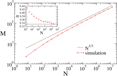
Figure 1: The average number of surviving particles $M$ versus system size $N$ for equal populations. The inset shows the quantity $\alpha\equiv d\ln M/d\ln N$ versus $N$. Fitting the data to the powerlaw $M\sim N^{\alpha}$ in the range for $N>10^{4}$ yields the exponent $\alpha=0.34$.

For single-species annihilation, it was found that the bulk of the reaction events occur during the early phase. Furthermore, while rare additional annihilation events may occur in the late phase, the number of such reactions does not alter the scaling laws for the ultimate number of surviving particles. It is thus possible to estimate the final number of surviving particles by evaluating the solution to Eq. (6) when $V=N$ at time $t\sim T\sim N^{2/3}$. According to the above definitions, $M_{+}=\displaystyle\lim_{t\to\infty}n_{+}(t)$ and similarly, $M_{-}=\displaystyle\lim_{t\to\infty}n_{-}(t)$. We anticipate that

$$M_{+}\sim n_{+}(T),\qquad M_{-}\sim n_{-}(T)\,.$$ (9)

As discussed below, our numerical simulations confirm these behaviors for a wide range of initial conditions.

IV Equal Populations

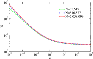
Figure 2: The scaling function $F(z)$ defined in (13). Shown is the scaled number of particles $F\equiv n/N^{1/3}$ versus the scaled time $z\equiv t/N^{2/3}$ for the case of equal number of particles for thee different system size.

We first consider the simplest case of equal populations, $\Delta=0$. Since the number difference is conserved, the two populations are identical $n_{+}=n_{-}=n/2$ with $n=n_{+}+n_{-}$ the total population. From the rate equations (6), the total population decays according to

$$\frac{dn}{dt}=-\frac{n^{2}}{2N},$$ (10)

during the early phase $t\ll T$. For the initial condition $n(0)=N$, the population decays as the inverse of time,

$$n(t)\sim N\,t^{-1}\,.$$ (11)

Let $M=\displaystyle\lim_{t\to\infty}n(t)$ be the average number of surviving particles. At the crossover time, the number of particles $M\sim n(T)$ is therefore (see figure 1)

$$M\sim N^{1/3}\,.$$ (12)

Our numerical simulations, shown in figure 1, confirm this scaling relation. As expected, the vast majority of annihilation events occur during the early phase when particles are inside the initially occupied region. A finite fraction of the particles that manage to survive at time $T$ persists forever.

The scaling relations (8) and (12) specify the typical time scale and the typical surviving population. These scaling laws fully characterize the time dependent behavior as the scaled population $n/M$ is a universal function of the scaled time $t/T$ for large systems (figure 2)

$$n(t)\sim N^{1/3}F\left(t/N^{2/3}\right)\,,$$ (13)

where $F(u)\sim u^{-1}$ for $u<<1$ and $F(u)\sim u^{0}$ for $u>>1$.

The average number of surviving particles (12) and the finite-size scaling behavior (13) agree with the corresponding behaviors for the single-species annihilation process. Hence, a finite and equal number of particles from each species survive the annihilation process when the initial populations are identical.

V The Critical Difference

In the rest of this study, we consider situations where the two populations differ in size, $\Delta>0$. In this section, we analyze the case where the population difference is fixed, that is, the disparity between the two populations is always equal to $\Delta$.

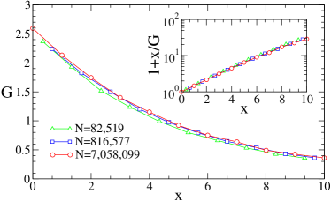
Figure 3: The scaling function $G(x)$, defined in equation (18). Shown is the scaled number of surviving minority particles $G\equiv M_{-}/N^{1/3}$ versus the scaled difference $x\equiv\Delta/N^{1/3}$ for the case of fixed population difference $\Delta$. Inset shows the function $1+x/G$, which according to Eq. (19) should increase exponentially with $x$.

Since the population difference is conserved, we may consider the minority population without loss of generality. By substituting $n_{+}=n_{-}+\Delta$ and $V=N$ into (6), we see that the minority population decays according to

$$\frac{dn_{-}}{dt}=-\frac{n_{-}(n_{-}+\Delta)}{N}\,.$$ (14)

The solution of this equation subject to the initial conditions $n_{-}(0)=N_{-}$ can be readily obtained,

$$n_{-}(t)=N_{-}\,\frac{\Delta}{N_{-}(e^{t\Delta/N}-1)+\Delta}\,.$$ (15)

Hereinafter, the dependence of $n_{-}(t)$ on $\Delta$ and $N$ is left implicit. We can recover the decay (11) from (15) in the limit $\Delta\to 0$.

The average number of surviving minority particles can be estimated by evaluating the minority population (15) at the crossover time (8),

$$M_{-}\sim N_{-}\,\frac{\Delta}{N_{-}(e^{\Delta/N^{1/3}}-1)+\Delta}\,.$$ (16)

According to this expression, the number of surviving minority particles grows algebraically with system size as in (12) when $\Delta\ll N^{1/3}$, but it decays exponentially when $\Delta\gg N^{1/3}$. Therefore, there is a critical difference, given by (1), and drastically different behaviors occur above and below this threshold,

$$M_{-}\sim\begin{cases}N^{1/3}&\Delta\ll\Delta_{c},\cr\Delta\,\exp\!\left(-c\,\Delta/N^{1/3}\right)&\Delta\gg\Delta_{c}.\end{cases}$$ (17)

Here, $c$ is a constant. For subcritical differences, a finite number of minority particles survive and the same hold for the majority species. Essentially, the system behaves as if the two populations are equal. However, for supercritical differences, extinction of the minority species is inevitable and the number of surviving majority particles is always equal to the initial difference. In the $N\to\infty$ limit, we have $M_{-}\to 0$ and $M_{+}\to\Delta$. Hence, the initial disparity dictates if the minority species survives or if it becomes extinct. Also, the final number of surviving particles fluctuates in the subcritical case but it is deterministic in the supercritical case.

We note that in the supercritical region, $\Delta\gg\Delta_{c}$, there is an additional characteristic time scale. Initially, the two populations are comparable and consequently, the decay (11) holds. However, the two populations are no longer comparable, $n_{-}(\tau)\sim\Delta$ at time $\tau\sim N/\Delta$. The majority population becomes dominant, $n_{+}\gg n_{-}$ when $t\gg\tau$, and according to (6), the minority population decays exponentially, $dn_{-}/dt=-\Delta n_{-}/N$, thereby leading to the exponential decay in (17).

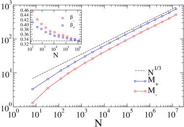
Figure 4: The surviving populations $M_{+}$ and $M_{-}$ versus system size $N$ for the special case $\Delta=N^{1/3}$. A fit of $M_{+}$ and $M_{-}$ to a power-law, $M_{\pm}\sim N^{\beta_{\pm}}$ in the range $N>10^{4}$ yields the exponents $\beta_{+}=0.34$ and $\beta_{-}=0.35$ respectively. The inset shows the quantity $\beta_{\pm}\equiv d\ln M_{\pm}/d\ln N$ versus $N$.

Numerically, we can confirm that the critical difference (1) characterizes the final population $M_{-}$. The scaled number $M_{-}/N^{1/3}$ becomes a universal function of the scaled difference $\Delta/N^{1/3}$ in the large-$N$ limit (figure 3)

$$M_{-}\sim N^{1/3}\,G\left(\Delta/N^{1/3}\right)\,.$$ (18)

The underlying scaling function is simply

$$G(x)=\frac{x}{e^{c\,x}-1}\,.$$ (19)

Results of our numerical simulations support this functional form as well (see inset in figure 3). The limiting behaviors of the scaling function are

$$G(x)\sim\begin{cases}1&x\ll 1\cr x\,e^{-c\,x}&x\gg 1\,.\end{cases}$$ (20)

The small-$x$ behavior shows that the problem reduces to the equal population case in the subcritical regime. The large-$x$ behavior reflects the extinction in the supercritical regime.

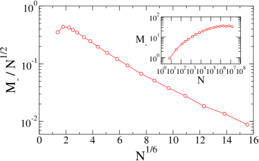
Figure 5: The normalized population $M_{-}/N^{1/2}$ versus $N^{1/6}$ for the special case $\Delta=N^{1/2}$. The inset shows the surviving population $M_{-}$ versus system size $N$.

To further verify the predictions of (16), we examined two special cases: $\Delta=N^{1/3}$ and $\Delta=N^{1/2}$. In the first case, which corresponds to the critical difference, we can confirm that $M_{+}\sim M_{-}\sim N^{1/3}$ (figure 4). In the second case, which is typical for equal initial concentrations, we expect a stretched exponential decay with a rather small characteristic exponent

$$M_{-}\sim\sqrt{N}\,\exp\!\left(-c\,N^{\frac{1}{6}}\right)\,.$$ (21)

Our numerical simulations are consistent with this behavior, despite the fact that $M_{-}$ grows with system size over the range of system sizes we probed numerically.

VI Equal Concentrations

We now consider the situation where the initial concentrations are equal. In this case, we have $N_{+}/N\to 1/2$ and $N_{-}/N\to 1/2$ in the limit $N\to\infty$. The disparity between the two populations is a fluctuating quantity, characterized by the typical difference $\Delta\sim N^{1/2}$. Moreover, the difference is normally-distributed and fully characterized by the distribution

$$P(\Delta)=\left(\frac{1}{2\pi N}\right)^{1/2}\exp\left(-\frac{\Delta^{2}}{2N}\right)\,.$$ (22)

We are interested in the average number of surviving particles $M_{+}$ and $M_{-}$, where the average is performed over all initial conditions and all realizations of the annihilation process.

The scaling law for $M_{+}$ in (3) follows from conservation of the number difference. As discussed in Section II, the initial difference provides a lower bound for the final number of majority particles, $M_{+}\geq\Delta$. For equal concentrations, $\Delta\sim N^{1/2}$, and according to (1) the system is typically in the supercritical regime. Consequently, the majority is dominant and $M_{+}\sim N^{1/2}$.

The scaling law for $M_{-}$ can also be obtained using heuristic arguments. According to equation (17), the minority population disappears when $\Delta\gg N^{1/3}$, but some minority particles do remain when $\Delta\ll N^{1/3}$. For equal concentrations, initial conditions of the former type occur with high probability, but initial conditions of the latter type may still be realized with a small probability. To estimate this small probability we conveniently replace the Gaussian in (22) with a uniform distribution with support in the compact interval $[-N^{1/2}:N^{1/2}]$. The initial difference is subcritical with probability $\sim N^{-1/2}\times\Delta_{c}\sim N^{-1/6}$. Therefore, the average size of the surviving minority population is $M_{-}\sim N^{-1/6}\times N^{1/3}\sim N^{1/6}$.

Thus, there are two different scaling laws for majority and minority survivors, $M_{+}\sim N^{1/2}$ and $M_{-}\sim N^{1/6}$. Yet neither of these behaviors resembles the scaling behavior (2) when the populations are equal. These two scaling relations give the survival probability of a majority particle, $S_{+}\sim N^{-1/2}$, and that of a minority particle, $S_{-}\sim N^{-5/6}$. The former survival probability increases by a factor $\sim N^{1/6}$, while the latter decreases by a similar factor when compared with the equal population case where $S_{+}\sim S_{-}\sim N^{-2/3}$.

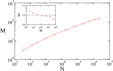
Figure 6: The average number of surviving minority particles $M_{-}$ versus $N$ for the equal concentration case. The inset shows the quantity $\beta_{-}=d\ln M_{-}/d\ln N$ versus $N$.

The surviving minority population may also be obtained by calculating the weighted average $\int_{0}^{\infty}d\Delta P(\Delta)M_{-}$ with $M_{-}$ given in (16). To estimate this integral, we use (16) to separate contributions corresponding to the subcritical phase and the supercritical phase,

$$M_{-} \sim \int_{0}^{N^{1/3}}d\Delta\left(\frac{1}{2\pi N}\right)^{1/2}\!\!N^{1/3}\,\exp\left(-\frac{\Delta^{2}}{2N}\right)\,$$

$$+ \int_{N^{1/3}}^{\infty}d\Delta\left(\frac{1}{2\pi N}\right)^{1/2}\!\!\Delta\,\exp\left(-\frac{\Delta^{2}}{2N}-\frac{\Delta}{N^{1/3}}\right)\,.$$

The first integral, which corresponds to the subcritical phase, is much larger than the second one, and indeed it gives $M_{-}\sim N^{1/6}$ . Our numerical simulations show that $M_{-}\sim N^{\beta_{-}}$ with $\beta_{-}<1/3$ (figure 6), but the exponent $\beta_{-}$ converges very slowly to the asymptotic value. While we are unable to provide direct numerical evidence for $\beta_{-}=1/6$, when taken as a whole, the rest of our simulation results do support this theoretical prediction.

We stress that the algebraic behavior $M_{-}\sim N^{1/6}$ characterizes an average over all realizations of the stochastic process and over all initial conditions. The initial difference $\Delta$ fluctuates from realization to realization and it is governed by the distribution (22). Once the initial conditions are set, the fate of the system is determined from the initial difference $\Delta$. There is a critical threshold $\Delta_{c}\sim N^{1/3}$. Below this threshold, $\Delta\ll\Delta_{c}$, a finite number of particles from both the majority and the minority survive ad infinitum and $M_{-}\sim M_{+}\sim N^{1/3}$. Above this threshold, however, all minority particles are annihilated and a finite number of majority particles survive: $M_{-}\to 0$ and $M_{+}\sim\Delta$.

Clearly, there are wild fluctuations from realization to realization. In the most probable scenario, the minority species goes extinct, but there are rare cases where the minority species survives and its population is comparable with that of the majority species. One way to characterize these fluctuations is through moments of the fluctuating number of minority survivors, $n_{-}(\infty)$. It is simple to generalize (VI) and find a continuous spectrum of scaling exponents that characterizes these moments

$$\langle n_{-}(\infty)^{m}\rangle\sim N^{\frac{2m-1}{6}}\,.$$ (24)

The decaying zeroth moment reflects that initial conditions with $\Delta\sim N^{1/3}$ are realized with probability $N^{-1/6}$. The behavior of large moments is controlled by the scaling law (2) for equal populations.

VII Monte Carlo Algorithms

Numerical simulations of two-species annihilation with a finite, yet large, number of particles are challenging for multiple reasons. First, the system is three dimensional. Even sophisticated Monte Carlo algorithms sb , developed recently, have not been able to produce numerical verification of the decay $c\sim t^{-3/4}$ in unbounded systems because the convergence to the ultimate asymptotic behavior is extremely slow bulatov . Second, large memory is required because particles may escape far outside the initially occupied domain. Third, the computing time is large because the very last annihilation event is unknown apriori and it fluctuates greatly from one realization to another. Knowledge of the time scale (8) is helpful with respect to this third challenge, and we run our simulation to time $t_{f}$ much larger than this scale, $t_{f}\propto 10^{4}\times N^{2/3}$.

In our numerical simulations, $N$ sites that fall within a fixed distance from the origin are occupied initially, but all remaining lattice sites are vacant. In each elementary simulation step, one randomly-selected particle moves to a randomly-selected nearest neighbor. If the target site contains a particle of the opposite type, the two particle are removed from the system. Time is augmented by the inverse number of remaining particles after each such elementary simulation step. We used two different algorithms to simulate this process. The two implementations differ in one respect only: in the first algorithm we do allow multiple occupancy, but in the second, we restrict occupancy to one particle per site. In the first implementation each of the $N$ sites are occupied by one majority particle and one minority particle but then $\Delta$ randomly-selected minority particles are removed from the system. In the second implementation each of the $N$ sites are occupied by a single particle. These two implementations yield very similar results which become essentially indistinguishable for large systems.

Our first simulation method is a brute force algorithm in which a one-dimensional array is used to keep track of each particle’s location. The advantage of this algorithm is that the memory required scales linearly with the initial number of particles $N$. However, the number of operations per unit time grows quadratically with the total number of active particles. This algorithm performs surprisingly well because most reaction events occur in the early phase, and in particular, the number of required operations scales as ${\cal O}(N^{2}\ln N)$ in the subcritical phase bk . We used this straightforward algorithm to produce the results shown in figures 1-5 and in figure 7.

Our second algorithm is more sophisticated in that it is efficient in both computation time and memory. To optimize the number of operations, we implement the standard approach for simulating diffusion-controlled reaction processes. Particles occupy an actual three-dimensional lattice and each lattice site contains a “pointer” to the particle occupying it such that one does not need to search through all particles in each move. With this approach, the number of operations per unit time scales linearly with the number of active particles. To optimize memory use, we take advantage of the fact the system becomes sparse with time. We thus map every lattice site in our very large array to a much smaller array using a hash function clrs ; sa . This approach allows us to simulate a large system with much less memory than would be needed if we stored the entire original lattice, and yields a speed up of up to a factor $10$ for $N\approx 10^{6}$. Results of this simulation algorithm are shown in Fig. 6.

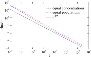
Figure 7: The reaction rate $-dn/dt$ versus time $t$ for the case $N=7,153$.

Our basic assumption, stated in equation (9), is that the number of surviving particles at time $T\sim N^{2/3}$ yields the correct scaling behavior for the surviving populations. To further test this assertion, we examined the reaction rate at late times. According to the rate equation (6) and the confining volume in (7), we expect $dn_{+}/dt\sim n_{+}n_{-}/t^{3/2}$. Our simulations confirm this behavior for both equal populations and equal concentrations. Hence, the residual correction to the ultimate number of surviving particles decays algebraically, $n(t)-M\sim t^{-1/2}$, and from this behavior it is simple to show that the total number of reaction events in the late-time regime $t\gg N^{2/3}$ is small enough so that (9) holds.

VIII General Spatial Dimensions

We now briefly discuss the behavior in general spatial dimensions; we restrict our attention to the equal concentration case and dimensions $d>2$ where the final state is nontrivial. It is straightforward to generalize the main results (1) and (3) to arbitrary dimension by replacing the characteristic time scale in (8) with $T\sim N^{2/d}$. The critical difference grows algebraically with the number of particles,

$$\Delta_{c}\sim N^{\delta}\qquad{\rm with}\qquad\delta=\frac{d-2}{d}\,,$$ (25)

when $d>2$. The surviving majority population exhibits two regimes of behavior

$$M_{+}\sim N^{\beta_{+}},\qquad\beta_{+}=\begin{cases}\frac{1}{2}&d\leq 4\cr\frac{d-2}{d}&4\leq d\,.\cr\end{cases}$$ (26)

The behavior agrees with (3) below the critical dimension, and the behavior coincides with that of single-species annihilation above the critical dimension. Finally, the surviving minority population exhibits three regimes of behavior

$$M_{-}\sim N^{\beta_{-}},\qquad\beta_{-}=\begin{cases}0&d\leq\frac{8}{3},\cr\frac{3d-8}{2d}&\frac{8}{3}\leq d\leq 4,\cr\frac{d-2}{d}&4\leq d\,.\cr\end{cases}$$ (27)

Interestingly, the quantity $M_{-}$ does not grow with system size below the lower critical dimension $d<8/3$ kr . However, the two surviving populations are comparable, and both are much larger than the initial difference $\Delta\sim N^{1/2}$ above the upper critical dimension, $d>4$.

IX conclusions

To summarize, we studied diffusion-controlled two-species annihilation in an unbounded space with a finite number of particles. Specifically, we addressed initial conditions where a finite number of particles is confined to a compact domain. We found that the disparity between the two populations controls the behavior. When the disparity is small enough, the two populations remain comparable throughout the reaction process, and a finite number survives the annihilation process. These particles manage to escape far outside the initial domain. However, when the initial disparity is large enough, the minority population becomes extinct while a finite number of majority particles survives. We used the rate equation approach to obtain a number of scaling laws for equal initial populations and for equal initial concentrations. Our numerical simulations support the theoretical predictions.

Our study focused on the most interesting case of three dimensions which is below the critical dimension $d_{c}=4$ for a homogeneous infinite-particle systems krb . For such systems, spatial correlations spontaneously develop and the result is a mosaic of $A$-rich and $B$-rich domains. These correlations play a crucial role and consequently, predictions based on the mean-field rate equations do not hold in three dimensions. The qualitative behavior is quite different when the number of particles is finite. No matter how large the initial number of particles is, the system remains well-mixed and spatial correlations are not strong enough to affect the scaling behavior. As a result, the rate equation predictions hold for finite systems fds .

Survival occurs only when $d>2$ and in some sense this escape phenomena is counter to the behavior when the number of particles is infinite. In an infinite system, the reaction rate is smaller in low dimensions whereas in a finite system, the total number of reaction events is smaller in high dimensions. Hence, the system size and dimensionality generally compete in reaction-diffusion processes as both affect the survival probability.

Our study highlights the serious challenge of developing theoretical tools for describing strongly interacting particle systems such as reaction-diffusion processes involving a large but finite number of particles. Existing theoretical methods are inadequate to handle such problems. As a rather straightforward extension of our work one may investigate two-species annihilation with unequal initial concentrations where according to (17), the survival probability of minority particles decays as a stretched exponential, $S_{-}\sim\exp(-{\rm const.}\times N^{2/d})$. Finally, we mention that it would be interesting to investigate another basic reaction-diffusion process, Brownian coagulation mvs ; sc , for initial conditions with a finite number of clusters.

References

- (1) P. L. Krapivsky, S. Redner and E. Ben-Naim, A Kinetic View of Statistical Physics (Cambridge University Press, Cambridge, 2010).
- (2) U.C. Täuber, Critical Dynamics (Cambridge University Press, Cambridge, 2014).
- (3) A. J. Bray, Adv. Phys. 43, 357 (1994).
- (4) D. Dhar, Physica A 263, 4 (1999).
- (5) J. P. Sethna, K. A. Dahmen, and C. R. Myers, Nature 410, 242 (2001).
- (6) P. Le Doussal and K. J. Wiese, Phys. Rev. E 88, 022106 (2013).
- (7) A. A. Ovchinnikov, S. F. Timashev and A. A. Belyi, Kinetics of Diffusion Controlled Chemical Processes (Nova Science Pub. Inc., 1989).
- (8) D. ben-Avraham and S. Havlin, Diffusion and Reactions in Fractals and Disordered Systems (Cambridge University Press, Cambridge, UK, 2000).
- (9) U. C. Tauber, M. Howard, and B. P. Vollmayr-Lee, J. Phys. A 38, R79 (2005).
- (10) K. Krebs, M. P. Pfannmuller, B. Wehefritz, and H. Hinrichsen, J. Stat. Phys. 78, 1429 (1995).
- (11) G. Foltin, K. A. Dahmen, and N. M. Shnerb, arXiv:cond-mat/0005015.
- (12) P. Argyrakis and R. Kopelmann, Phys. Rev. A 41, 2121 (1990).
- (13) C. Domain, C. S. Becquart, and L. Malerba, J. Nucl. Mater. 335, 121 (2004).
- (14) A. Savara and E. Weitz, Jour. Phys. Chem. C 114, 20621 (2010).
- (15) M. E. J. Newman and G. T. Barkema, Monte Carlo Methods in Statistical Physics, (Oxford University Press, Oxford, 1999).
- (16) M. Cross and H. Greenside, Pattern Formation and Dynamics in Nonequilibrium Systems (Cambridge University Press, Cambridge, 2009).
- (17) E. Ben-Naim and P. L. Krapivsky, J. Phys. A 49, 504004 (2016).
- (18) E. Ben-Naim and P. L. Krapivsky, J. Phys. A 49, 504005 (2016).
- (19) D. Toussaint and F. Wilczek, J. Chem. Phys. 78, 2642 (1983).
- (20) Ya. B. Zeldovich, Zh. Tekh. Fiz. 19, 1199 (1949); Ya. B. Zeldovich and A. S. Mikhailov, Sov. Phys. Usp. 30, 23 (1988).
- (21) S. F. Burlatsky, Teor. Eksp. Khim. 14, 52 (1978).
- (22) Ya. B. Zeldovich and A. A. Ovchinnikov, Chem. Phys. 28, 215 (1978).
- (23) S. F. Burlatsky, A. A. Ovchinnikov, and G. S. Oshanin, Sov. Phys. JETP 68, 1153 (1989).
- (24) D. ben-Avraham, J. Chem. Phys. 88, 941 (1988).
- (25) M. Bramson and J. L. Lebowitz, J. Stat. Phys. 65, 941 (1991).
- (26) L. Galfi and Z. Racz, Phys. Rev. A 38, 3151 (1988).
- (27) E. Ben-Naim and S. Redner, J. Phys. A 25, L575 (1992).
- (28) F. Leyvraz and S. Redner, Phys. Rev. A 46, 3132 (1992).
- (29) I. Ispolatov and P. L. Krapivsky, Phys. Rev. E 53, 3154 (1996).
- (30) E.V. Albano, J. Phys. Chem. C 115, 24267 (2011).
- (31) C.P Haynes, R. Voituriez, and O. Benichou, J. Phys. A 45, 415001 (2012).
- (32) R. Dandekar, arXiv:1602.05483.
- (33) B. M. Shipilevsky, Phys. Rev. E 95, 062137 (2017).
- (34) P. Mörters and Y. Peres, Brownian Motion (Cambridge: Cambridge University Press, 2010).
- (35) M. V. Smoluchowski, Phys. Z. 17, 557 (1916); Z. Phys. Chem. 92, 129 (1917); ibid 92, 155 (1917).
- (36) Y. Shafrir and D. ben-Avraham, Phys. Lett. A 278, (2001).
- (37) T. Oppelstrup, V. V. Bulatov, A. Donev, M. H. Kalos, G. H. Gilmer, and B. Sadigh, Phys. Rev. Lett. 97, 230602 (2006); Phys. Rev. E 80, 066701 (2009).
- (38) T. H. Cormen, C.E. Leiserson, R.L. Rivest, C. Stein, Introduction to Algorithms (MIT press, Cambrdidge, 2009).
- (39) E.H. Sabbar and J.G. Amar, Surf. Sci. 664, 38 (2017).
- (40) P. L. Krapivsky and S. Redner, J. Phys.: Condens. Matter 19, 065119 (2007).
- (41) S. Chandrasekhar, Rev. Mod. Phys. 15, 1 (1943).