Variable selection with genetic algorithms using repeated cross-validation of PLS regression models as fitness measure

Abstract

Genetic algorithms are a widely used method in chemometrics for extracting variable subsets with high prediction power. Most fitness measures used by these genetic algorithms are based on the ordinary least-squares fit of the resulting model to the entire data or a subset thereof. Due to multicollinearity, partial least squares regression is often more appropriate, but rarely considered in genetic algorithms due to the additional cost for estimating the optimal number of components.

We introduce two novel fitness measures for genetic algorithms, explicitly designed to estimate the internal prediction performance of partial least squares regression models built from the variable subsets. Both measures estimate the optimal number of components using cross-validation and subsequently estimate the prediction performance by predicting the response of observations not included in model-fitting. This is repeated multiple times to estimate the measures’ variations due to different random splits. Moreover, one measure was optimized for speed and more accurate estimation of the prediction performance for observations not included during variable selection. This leads to variable subsets with high internal and external prediction power.

Results on high-dimensional chemical-analytical data show that the variable subsets acquired by this approach have competitive internal prediction power and superior external prediction power compared to variable subsets extracted with other fitness measures.

Keywords: Variable selection, Genetic algorithm, Cross-validation, QSPR, Prediction performance

1 Introduction

Building models from chemical-analytical data suitable for predicting future observations is challenging and often requires the reduction of dimensionality. In lots of situations, too many variables can dramatically increase the noise in the data and thereby decrease the descriptive and predictive power of a model. However, deciding which variables carry most of the relevant information highly depends on the problem. Variables that can represent the data very well may be less important for predicting future observations and vice versa. Thus, most variable selection procedures are designed for specific problem settings and data structures.

Predicting future observations is a prevalent use case for models of chemical-analytical data. Quantitative structure-property relationship models (QSPR), for instance, relate structural data (molecular descriptors) to properties of the compounds. Predicting the properties of compounds when only the molecular descriptors are known is an important use of these models. QSPR data often comprises a huge number of molecular descriptors but the property is known only for a few compounds. As many of these molecular descriptors are also highly correlated, PLS regression models^{19, 23} are frequently used to fit the model to the data. Therefore, in order to fully specify the PLS regression model, the complexity of the PLS model must be estimated. This poses the necessity of estimating the number of PLS components and finding the molecular descriptors most important to predicting the property at question for other compounds simultaneously.

Once the use of the model and the structure of the data is known, a validation criterion that can assess the quality of the model with respect to this intended use must be specified. The validation criteria discussed in this paper have the sole purpose of finding variable subsets with high prediction power. The need to estimate the number of PLS components complicates the validation even further. Repeated double cross-validation (rdCV)⁷ is a useful method for validating the prediction power of PLS regression models. As discussed by Gramatica ¹⁰, internal and external prediction power have to be differentiated as well as considered when choosing the validation criterion. Due to its favorable properties, rdCV will be used as reference for the internal prediction performance of PLS models throughout this paper.

Many different strategies for variable selection have been intensively studied in the chemometrics literature. Simple methods for variable selection are based on the empirical correlation coefficient between the covariates and the response variable. Another class of methods is stepwise regression. A single variable is added/removed to/from the model such that a previously defined model performance criterion is optimized in each step. As ordinary least-squares regression estimates are used for most stepwise regression approaches, multicollinearity and too many covariates are a strong limitation for these methods⁸. A comprehensive listing of these simple variable selection methods is given in Varmuza et al. ²⁰. Recently, an enhanced version of well-known sequential replacement methods was published¹², which gives very promising results for QSPR models and is also quite fast to compute. Other methods directly use PLS regression models to search for variable subsets. One form of these methods is based on significance tests, for instance by iteratively removing variables that are insignificant according to a t-test on the estimated coefficients²².

Genetic algorithms (GA) are another prevalent class of methods used for variable selection in chemometrics. ¹⁶ As GAs are highly adaptable, different forms were used in research in the past. However, all methods share the need for an easy to compute internal fitness measure. As this fitness measure has to be calculated for many different models, its computational speed is of high priority. Too complex validation criteria take long time to compute and therefore simple, fit-based criteria where the regression estimates are only calculated once for the entire data are dominant in the literature. The mature GA in Gramatica et al. ¹¹ uses the coefficient of determination ($R^{2}$), a fit-based criterion, calculated from the leave-one-out (LOO) residuals obtained from an OLS regression model. These LOO residuals can be easily calculated from an OLS regression model that is once fit to the entire (training) data. However, as multicollinearity is a big issue for OLS regression, the risk is that variables that are highly correlated with each other are removed before employing the GA. Predictive abilities of PLS regression models have already been considered in genetic algorithms.¹⁵ However, to simplify computation, the number of optimal PLS components was estimated only once using all variables, and the chosen criterion to be optimized was the cross-validated explained variance ($Q^{2}$). A similar approach² was to fit a PLS regression model to a fixed training set and validate the prediction power on a fixed model test set within the GA. Both methods do not account for inherent variation between different cross-validation segmentation as well as splits into training and validation sets. In this paper we propose new measures of prediction power to be used within GAs that take the variation between different splits of the data into consideration.

We will emphasize the need of accurate estimation of the prediction power within the genetic algorithm. First, the considered validation criteria are discussed in detail. What follows is a short description of the genetic algorithm used for the comparison of the validation criteria. After comparison of the variable subsets extracted by using the different validation criteria in the GA, the best performing models will be put into relation with variable subsets proposed in previous papers.

2 Validation

To compare two variable subsets, the purpose of the resulting model and the properties of the data must be taken into account. In chemometrics, the number of covariates is often a multitude of the sample size and many of these covariates can be highly correlated. Also, as prediction power of the model is of major interest, the complexity of the model has to be optimized. Partial least squares (PLS) regression was designed to cope with these issues. Both, the covariates $\mathbf{X}\in\mathbb{R}^{N\times p}$ and the response $\mathbf{y}\in\mathbb{R}^{N}$ are assumed to be generated by the same latent variables (components). With the number of PLS components $A$, the complexity of the model can be adjusted to avoid overfitting and increase prediction power. Due to these favorable properties, PLS regression is a prevalent tool in chemometrics^{23, 21}.

2.1 Estimating the Number of PLS Components

As the number of PLS components determines the complexity of the resulting model and is generally not known beforehand, it must be chosen sensibly. Too few components will result in an inappropriate model that is not able to fit the essential structure of the data, while too many components will result in a model overfitted to the available samples. Considering this, cross-validation (CV) is a widely used method for estimating the optimal number of components.

Cross-validation works by repeatedly fitting the model to a portion of the data and validating the prediction performance on the other part of the data. First, the data is split randomly into $K$ almost equally sized segments. $K-1$ segments are then used to fit PLS models with one to the maximum of $A_{\mathrm{max}}$ components. These fitted PLS models are used to predict the values from the left out segment (validation set). When this procedure has been repeated $K$ times, such that each segment takes the role of the validation set exactly once, $A_{\text{max}}$ predicted values $\hat{y}_{i}^{(a)}$ are available for every observation $y_{i}$. Let $\mathcal{J}_{k}$ denote the indices of observations belonging to segment $k$, $k=1,\dotsc,K$. The mean squared error of prediction $\text{MSEP}_{a}$ can be calculated for each number of components $a$ according to

$$\text{MSEP}_{a}=\frac{1}{K}\sum_{k=1}^{K}\frac{1}{|\mathcal{J}_{k}|}\sum_{j\in\mathcal{J}_{k}}\left(y_{j}-\hat{y}_{j}^{(a)}\right)^{2},\quad a=1,\dotsc,A_{\text{max}}.$$ (1)

$\text{MSEP}_{a}$ guides the search for the optimal number of components. $A_{\text{opt}}$ can now be chosen as the number of components that results in the minimal $\text{MSEP}_{a}$ or by other heuristics. An often used strategy is taking the smallest number of components that results in a $\text{MSEP}_{a}$ that is still less than the minimal $\text{MSEP}_{a}$ plus one standard error (the one standard error rule as described in Hastie et al. ¹³, Figure 3.7), given by

$$A_{\text{opt}}:=\min\left\{a:\text{MSEP}_{a}\leq\text{MSEP}_{m}+\frac{\text{SE}_{m}}{\sqrt{K}}\right\}\quad\text{with }m=\operatorname*{arg\,min}_{a}\text{MSEP}_{a},$$ (2)

whereas the standard error $SE_{a}$ of the MSEP for the model with $a$ components is defined as

$$\text{SE}_{a}=\sqrt{\frac{1}{K-1}\sum_{k=1}^{K}\left(\text{MSEP}_{a}-\frac{1}{|\mathcal{J}_{k}|}\sum_{j\in\mathcal{J}_{k}}\left(y_{j}-\hat{y}_{j}^{(a)}\right)^{2}\right)^{2}}.$$ (3)

Once the optimal number of components is estimated, validation of the model for the desired use is mandatory. For validating the prediction power of the model, an independent set of observations is desirable but seldom extant. To circumvent the need of an independent set of observations, different strategies have been proposed in the literature. Measures acquired during the CV for model-calibration are too optimistic,⁷ so other measures to validate the model have to be used.

The easiest and fastest way to validate any model is to quantify how well the model fits the data. No independent data set is needed for validation and the computational burden is very low as only one model with $A_{\text{opt}}$ number of components has to be fit to the data. Prominent methods to assess the model-fit are well-known information criteria like Akaike’s information criterion (AIC) and the Bayes information criterion (BIC) or the coefficient of determination ($R^{2}$). Because $R^{2}$ gets larger the more covariates are used in the model, the adjusted $R^{2}$ is usually preferred when models with different numbers of predictors are to be compared as it penalizes greater numbers of predictors. However, if prediction power of the model is of primary interest, fit-based criteria are not able to quantify the desired properties.

2.2 Repeated Double Cross-Validation

Especially when the number of available observations in the data set is small, which is often the case for QSPR models,²⁰ resampling methods are the only way to estimate the prediction performance of the model.¹⁰

Filzmoser et al. ⁷ proposed the repeated double cross-validation (rdCV) strategy, an extension to double cross-validation,¹ as reliable estimate for the prediction performance of PLS regression models. Similar to double cross-validation it consists of an outer CV loop and an inner CV loop. In the outer CV loop, the data are split into $S$ segments. The calibration set consist of $S-1$ segments and the remaining segment is used as test set (see Figure 1). Using the calibration set, the optimal number of components $A_{\text{opt}}$ is estimated in the inner CV loop. The model with $A_{\text{opt}}$ components is then fit to this calibration set. The fitted model is finally used to predict the response in the test set. This is repeated such that each of the $S$ outer segments is used as test set exactly once, hence for every observation $y_{i}$ a predicted value $\hat{y}_{i}$ is available and the information of $y_{i}$ and $\mathbf{x}_{i}$ is not used for this prediction. With these predictions the Standard Error of Prediction (SEP) can be calculated as

$$\begin{split}\text{SEP}&=\sqrt{\frac{1}{N-1}\sum_{i=1}^{N}\left(y_{i}-\hat{y}_{i}-\text{bias}\right)^{2}}\\ \text{where }\text{bias}&=\frac{1}{N}\sum_{i=1}^{N}\left(y_{i}-\hat{y}_{i}\right).\end{split}$$ (4)

A similar concept and also often used for model assessment is the Root Mean Squared Error of Prediction (RMSEP). It is given by

$$\text{RMSEP}=\sqrt{\frac{1}{N}\sum_{i=1}^{N}(y_{i}-\hat{y_{i}})^{2}}$$ (5)

and can be expressed in terms of the standard error of prediction $\text{RMSEP}=\sqrt{\frac{N-1}{N}\text{SEP}^{2}+\text{bias}^{2}}$.

Although double cross-validation gives a reliable estimate of the prediction error,¹ the segmentations in both the outer and the inner CV loop is random and hence the estimated SEP is a random quantity as well. To get viable information about it’s variance, a single value is insufficient. In rdCV, the procedure is therefore repeated with different splits in the outer as well as in the inner CV loop. A final estimate for the prediction performance is then the arithmetic mean of all SEP replications.

The outer and inner CV loop make the rdCV estimate computationally expensive, which can be a huge handicap when many different models need to be validated. Also, in case of data sets with only a small number of observations, the single segments and thus the test set in rdCV contains only a few observations ($N_{\text{test}}$ is very small). As this can lead to inappropriate estimates and long computation times, a simplified version is introduced.

2.3 Simple Repeated Cross-Validation

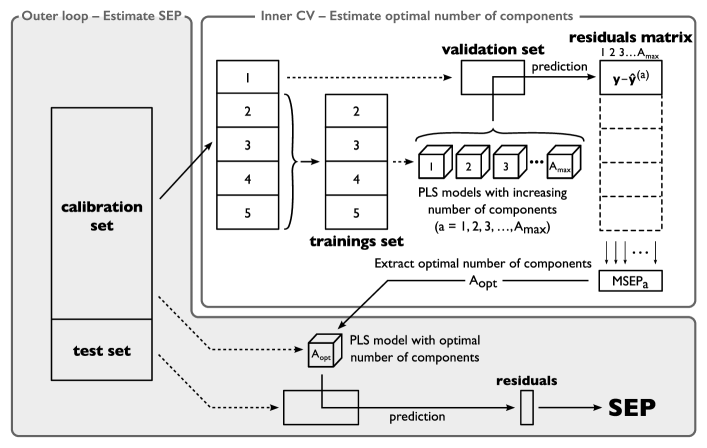
Figure 1: Scheme of a single replication for simple repeated cross-validation (modified from Varmuza et al. ²⁰, p. 3)

Simple repeated cross-validation (srCV) is a simplified and hence faster version of rdCV. In contrast to rdCV, the outer loop is not a cross-validation loop, but the data set is only split at random into a calibration set and a test set. The calibration set is again used to estimate the optimal number of components according to the scheme described in the above section. Likewise, the resulting model with $A_{\text{opt}}$ components is then fit to the complete calibration set. This fitted model is subsequently used to predict the responses from the test set. Finally, the standard deviation of the resulting residuals is used as an estimate for the SEP.

As with rdCV, the estimate varies with different splits into calibration and test sets. To assess the variability and to get a more reliable estimate for the SEP, the procedure is repeated multiple times with different splits into calibration and test set. The arithmetic mean of all replicated SEP values is taken as the final estimate of the prediction power.

The simplification engenders another advantage over rdCV. The size of the test set is not fixed to one segment of the outer cross-validation loop, but can be adjusted to include an arbitrary number of observations.

2.4 External Validation

According to Gramatica ¹⁰, external and internal validation methods must be differentiated. Although above methods use one part of the data for fitting the model(s) and the other part for assessing the prediction power, due to the replications, information from the entire data is used nevertheless. Therefore, they are considered as internal validation criteria and tend to overestimate the prediction power. To estimate the prediction power for totally new – external – observations, the model has to be validated with data that was never used during model selection. This is particularly challenging when only few observations are available.

3 Genetic Algorithm

To compare the different validation criteria in the variable selection setting, a simple genetic algorithm (GA) was used. Genetic algorithms⁹ are a very general class of methods for finding a global optimum in a large search space with no assumptions on the objective function, by combining a guided and a random search, mimicking strategies from evolution. To reduce the size of the search space and therefore the time complexity, only variable subsets within a minimum and maximum number of variables are considered. For this, a GA following the scheme described in Leardi ¹⁴ that supports all aforementioned validation criteria was implemented for the statistical software environment R¹⁷ and is available as package gaselect on CRAN.

Genetic algorithm terminology highly draws from genetics. Points in the search space are denominated as chromosomes and they are defined by their genes. Every chromosome has an associated fitness value that forms the objective function the GA optimizes. In GAs for variable selection, every possible variable subset is represented by a chromosome and the fitness of a chromosome is calculated with one of the validation criteria previously defined.

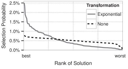
Figure 2: Impact of transforming the selection probabilities with the exponential function on exemplary fitness values. The left-most chromosome has the highest fitness and the right-most chromosome the lowest fitness. Without transformation, the selection probabilities for most chromosomes are similar, causing the algorithm to converge to the minimum at a slower rate.

The search starts by selecting a large number of different chromosomes and evaluating their fitness. Starting from this initial generation, evolution is imitated by randomly combining two chromosomes (mating) to form two offsprings and randomly adding/removing variables (mutation) to/from these offsprings. Like in evolution, chromosomes with higher fitness have a greater chance to be selected for mating and thus have a higher chance to produce offsprings. For selecting the chromosomes, the fitness $f(c)$ of chromosome $c$ is standardized by $f^{\ast}(c)=\frac{f(c)-\overline{f(c)}}{SD(f(c))}$ before the selection probabilities are assigned. As extremely bad chromosomes result in almost equal selection probabilities for all solutions, even for very good ones, the scaled fitness $f^{\ast}(c)$ is optionally transformed with the exponential function $f^{\ast\ast}(c)=exp\left(f^{\ast}(c)\right)$. Figure 2 shows the difference between $f^{\ast}(c)$ and $f^{\ast\ast}(c)$ in the selection probabilities of chromosomes in a generation with only few bad solutions present.

Once two chromosomes are selected, the mating process takes place. The two most common ways to combine two chromosomes are single crossover or uniform crossover.¹⁴ For single crossover, one gene is randomly selected as splitting point. The first offspring is formed by the genes left and including the selected gene from the first parent and the genes to the right of the selected gene from the second parent. The second offspring is formed in a similar fashion by exchanging the two parents’ roles. Uniform crossover randomly selects an arbitrary number of genes. The selected genes from the first parent and the non-selected genes from the second parent shape the first offspring. Again, by exchanging the role of the two parents, the second offspring is created.

To give the GA a chance to elude local optima, the offspring’s genes can mutate with a small probability. The number of mutated genes follows a double truncated geometric distribution with probability mass function shown in Figure 3 and given by

$$g(k)=\frac{p\left((1-p)^{2+k+l-2\max(l,k-u)}-(1-p)^{k+l-2\min(0,k)}\right)}{(p-2)(1-(1-p)^{1+u})(p-1+(1-p)^{l})}\quad k\in[l,u]$$ (6)

where $1-p$ is the mutation probability, $u$ ($>0$) is the upper truncation point and $l$ ($<0$) is the lower truncation point, hence the support of the distribution is between $l$ and $u$. The distribution needs to be truncated to guarantee that the number of variables stays between the set limits. This distribution arises as the difference between two truncated geometric distributed random variables,¹⁸ one with truncation point $u$ and the other one with truncation point $-l$. Thus, it is improbable that many genes mutate and the number of variables in a subset will never be outside the specified bounds.

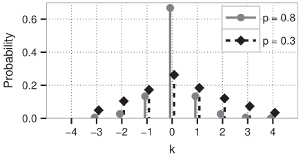
Figure 3: Probability mass function $g(k)$ of a truncated double geometric distribution with $l=-3$ and $u=4$.

The fitness of the new offspring has to be evaluated with a selected validation criterion. However, an offspring will not be accepted if it is a certain degree worse than the parent with the lower fitness, thus very bad combinations or mutations are discarded right away. The offspring will also be rejected if it is a duplicate of another chromosome in the offspring-generation. Consequently, a high level of diversity in the new generation is maintained and the average fitness of the population increases.

If an offspring is extraordinary fit it will join the elite. Elite chromosomes have the chance for mating in every generation, but if the group gets too large, the worst chromosome from the elite will be discarded.

When there are as many offsprings as there were chromosomes in the previous generation, these offsprings form the new generation and may produce offsprings themselves. The GA will stop once a predefined number of generations are generated. More details about genetic algorithms can be found in previously published literature.^{9, 21, 14}

The computationally most expensive step is to evaluate a chromosome’s fitness. To mitigate the computational burden, genetic algorithms can be parallelized to distribute the work load to multiple processing units. One way is to split the entire population into a number of completely independent subpopulations of smaller size. This could be extended to allow some chromosomes to switch the subpopulation at certain times. Another approach, implemented in the GA utilized to compare the validation criteria in this work, is to use one big population and distribute the mating, mutation, and evaluation step to multiple nodes. Every node produces a fixed number of offsprings according to the above steps, without need for interaction between the nodes and therefore almost no overhead caused by parallel computation.

We have implemented the SIMPLS algorithm⁴ to calculate the PLS regression estimates. As it is performed numerous times, we aggressively optimized the algorithm for single response models. As pointed out by Faber and Ferré ⁵, the SIMPLS algorithm is numerically quite unstable due to the orthogonality requirement for the loadings. To mitigate this problem, we employ the modified Gram-Schmidt (MGS) orthogonalization process, but avoided the recommended reorthogonalization due to the performance penalty. Thus, the algorithm may give inaccurate results for models with an extraordinary large number of components.

4 Applications

Performance of the validation criteria for variable selection is compared by checking the internal and external prediction power of the resulting variable subsets. Two real-life QSPR data sets will be used for this analysis.

Additionally to the rdCV and the srCV, two fit-based validation criteria are also considered in the following. The most naive approach is to use the BIC value

BIC $$=N\log(\text{RSS}/N)+p\log(N)$$ (7)

where RSS $$=\sum_{i=1}^{N}\left(y_{i}-\hat{y}_{i}\right)^{2}$$

obtained from an ordinary least squares fit to the entire data (denoted by $\text{BIC}_{\text{OLS}}$). This method is of course only applicable when the number of variables in the considered model is less than the number of observations and no pair of selected variables is perfectly collinear. In the examples considered in this paper, we always try to find models with only a few variables and therefore the only problem is multicollinearity. When the OLS estimate for a model can not be computed, the model is not considered further in the GA. The other fit-based method considered is the BIC value obtained from a PLS regression model, also fit to the entire data (denoted by $\text{BIC}_{\text{PLS}}$). The number of PLS components is estimated with the cross-validation procedure described above. We include these two methods to compare our proposed validation criteria to commonly used ones.

Performance of the new internal fitness measures is compared to the established fit-based fitness measures by employing them in the GA applied to two high-dimensional QSPR data sets. Both data sets have more variables than observations and multiple highly correlated variables. The validation criteria will be compared to each other and to results obtained in previously published papers ^{11, 20} concerned with these data sets.

4.1 Data sets

KOC data set.

Data of the soil sorption coefficient, normalized on organic carbon ($\mathrm{K_{\mathrm{oc}}}$) for $N=643$ heterogeneous organic compounds¹¹ with $p=1266$ molecular descriptors. Because the compounds are very heterogeneous, it is difficult to find variable subsets that give a good prediction for all different kinds of compounds.

PAC data set.

The GC retention index for $N=209$ polycyclic aromatic compounds (PAC) with $p=2688$ molecular descriptors.²⁰ This data set is particularly demanding for variable selection algorithms due to the very high number of variables, multicollinearity and comparatively few observations. In Varmuza et al. ²⁰ different variable selection procedures were used to find good variable subsets for prediction and their results will be compared to the results in this work.

4.2 Results

The GA described in the previous section is used with the different validation criteria to search for suitable variable subsets. For both data sets, the GA was employed with a population size of 4000 chromosomes and generated 300 generations. The three validation criteria using PLS regression models (rdCV, srCV, and $\text{BIC}_{\text{PLS}}$) were configured to estimate the optimal number of components with 10 CV segments (inner loop). The rdCV criterion was used with four outer CV segments, while the srCV criterion used 60 percent of the data for calibration and the other 40 percent as test set. Both criteria were employed with 30 replications. Due to the larger number of variables and therefore larger search-space, the mutation probability for the GA applied to the PAC data set was set to $0.5$ percent, compared to $0.25$ percent for the GA applied to the KOC data set. For the PAC data set, the GA was searching for variable subsets with 3 to 30 variables, whereas for the KOC data set, the number of variables was limited to 10.

Numerous variable subsets of the PAC data set give extremely large SEP values. The average fitness of the initial population is more than 4.5 times as large as the fitness of the final solution. Variable subsets from the KOC data set have similar properties, albeit less severe. As this has a significant influence on the chromosome selection during the GA, the fitness values have been transformed as outlined in the previous section.

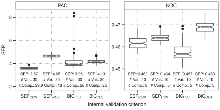
Figure 4: Distribution of the estimated SEP using the rdCV implementation provided by the R package chemometrics⁶ for variable subsets found with the GA using different internal validation criteria.

Internal prediction power was verified for the ten top ranked variable subsets (according to the used validation criterion) with the rdCV implementation provided in the R package chemometrics ⁶. The procedure was run with 50 replications, 10 inner and 4 outer CV segments using the kernelpls algorithm for PLS regression (“algorithm 1” in Dayal and MacGregor ³) as this algorithm is numerically more stable than SIMPLS. For rdCV and srCV, the results of the R procedure were very similar to the internal prediction power estimated by the GA.

Of these ten top ranked variable subsets, the SEP of the best subset according to the verified internal prediction power for each data set and validation criterion is shown as boxplot in Figure 4. Additionally, the size of the variable subset as well as the estimated optimal number of components is given in the graph. The variable subset for PAC found using rdCV as validation criterion gives the best results in terms of SEP. However, it is interesting that the two fit-based validation criteria result in variable subsets with a lower SEP than the srCV criterion. Moreover, the variability of the SEP of variable subsets extracted with the fit-based criteria is much higher than for the other two criteria. The notches of the boxes do not overlap, which is an indication that the differences of the medians are significant. All four validation criteria combined with the GA give significantly better variable subsets than the simple variable selection methods demonstrated in Varmuza et al. ²⁰. The best (in terms of rdCV) variable subset in Varmuza et al. ²⁰ leads to a SEP of approximately $5.6$, compared to the minimum SEP of $3.57$ reported here.

With regard to the internal prediction power of the variable subsets found for the KOC data set, the fit-based criterion using PLS regression models gives the best result. However, the SEP is only 1 percent smaller than the SEP of the variable subset found with rdCV and variability of the SEP is quite large. Such solutions which result in large SEP values for certain CV splits will less likely be considered by rdCV and srCV, as both criteria use the arithmetic mean over all different splits and are therefore more affected by these extreme values. Therefore, the internal prediction power of the variable subsets obtained with rdCV is very competitive.

A major weakness of the GA is immediately apparent from the found variable subsets: almost all variable subsets have the maximum allowed number of variables. The main reason for this is the very primitive mating procedure implemented in the GA. We do not take the number of variables of the parents into account before the mating takes place. Therefore, child chromosomes can have up to double the number of allowed variables. The excessive variables are randomly removed to constrain the number of variables to the specified range. Thus, a reasonable enhancement to the GA would be to take the number of variables of the parents into account prior to mating.

Visualization of the average and best SEP during the run of the genetic algorithm in Figure 5 supports the statement from above, that the average fitness increases over generations. The GA applied to the KOC data set could have been stopped earlier, as the fitness did not increase at all after the first 100 generations. However, unlike many other GAs, the utilized GA does not use any form of stopping criterion when the fitness is not improving anymore. Additionally, the graph shows that there exist multitudinous variable subsets which yield an extremely large SEP, underlining the need for transformation of the fitness $f(c)$ to $f^{\ast\ast}(c)$ when assigning the selection probabilities.

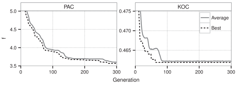
Figure 5: Progression of the average fitness and the fitness of the best chromosome over generations. Results taken from the GA run that resulted in the variable subset with the lowest SEP.

External prediction power of the variable subsets selected with the different criteria was estimated by applying the GA to a subset of the data (external training set) and calculating the root mean squared error of prediction for the predictions of the other part of the data (external validation set). For the PAC data set, 60 percent of the observations were randomly chosen to form the external training set. To get an estimate of the variability induced by the random split, we repeated the entire process 10 times. In the case of the KOC data set, we used the same 93 samples as in the paper by Gramatica et al. ¹¹ for variable selection and the other 550 samples for validation in order to make the results comparable.

Table 1: External prediction power of variable subsets extracted by the GA using different validation criteria for the two data sets.

Data set	Valid. criterion	No. obj. training	No. obj. validation	No. var.	No. comp.	RMSEP ext. training	RMSEP ext. validation	RMSEP total
PAC	$\text{SEP}_{\text{rdCV}}$	125	84	30	13 – 23	$3.33\pm 0.54$	$8.31\pm 1.2$	$5.66\pm 0.6$
PAC	$\text{SEP}_{\text{srCV}}$	125	84	30	9 – 17	$4.17\pm 0.23$	$7.33\pm 0.74$	$5.37\pm 0.44$	*
PAC	$\text{BIC}_{\text{PLS}}$	125	84	30	25 – 30	$2.8\pm 0.45$	$8.92\pm 0.79$	$5.83\pm 0.52$
PAC	$\text{BIC}_{\text{OLS}}$	125	84	30	26 – 30	$3.34\pm 0.74$	$8.9\pm 1.7$	$5.81\pm 0.95$
KOC	$\text{SEP}_{\text{rdCV}}$	93	550	10	4	$0.407$	$0.519$	$0.5$
KOC	$\text{SEP}_{\text{srCV}}$	93	550	10	4	$0.374$	$0.503$	$0.487$	*
KOC	$\text{BIC}_{\text{PLS}}$	93	550	10	8	$0.372$	$0.592$	$0.559$
KOC	$\text{BIC}_{\text{OLS}}$	93	550	10	8	$0.387$	$0.616$	$0.581$

The external training and external validation set are randomly chosen for the PAC data set, hence the median and median absolute deviation calculated from 10 runs are presented. The variable subset with the best external prediction power for each dataset is highlighted with an asterisk

In terms of external prediction power, the srCV validation criterion outperforms the other two criteria. As listed in Table 1, the rdCV criterion and the fit-based methods find variable subsets with better internal prediction power (RMSEP ext. training). However, the variable subsets extracted with the srCV criterion is superior when predicting observations that were not used during the GA to find the variable subset (RMSEP ext. validation) and when considering the RMSEP for all observations (RMSEP total). Moreover, variable subsets found with srCV tend to result in simpler PLS regression models with less numbers of components. We can also see that the RMSEP for the training data is significantly lower than the RMSEP for the validation set with all validation criteria, hence prediction power of the model is overestimated by all criteria. The simplifications in srCV were initially targeted to speed up the computations. However, by loosing the restrictions on the size of the test set, the validation criterion is able to estimate the external prediction power of the model more accurately.

The variable subsets found with srCV using only 93 samples from the KOC data set is very competitive. It is superior to the variable subsets reported in Gramatica et al. ¹¹ in terms of RMSEP for external as well as internal observations. Therefore, the RMSEP for the total data set is almost 10 percent lower than for the best performing subset reported in their paper ($\text{RMSEP}=0.532$).

Currently the major drawback of the proposed validation criteria is the high computation time required. The computations for each run were distributed to 32 threads and the times recorded (Figure 6). The simplifications in srCV from rdCV are very effective, decreasing computation time by more than 500 percent compared to rdCV. Of course, the simple fit based criteria are still significantly faster, but the resulting variable subsets are suboptimal. Also, as discussed above, the genetic algorithm generated 300 generations regardless of significant improvements between generations. The current GA implementation leaves room for many more improvements in terms of fitness of the solution as well as speed. For instance, a more sophisticated GA could stop the evolution as soon as the fitness does not improve significantly over some generations and therefore finish faster.

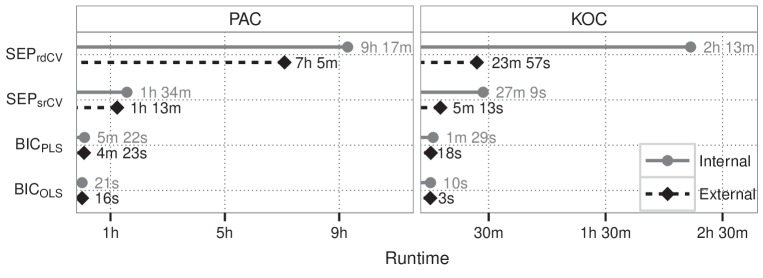
Figure 6: Runtime of the GA (distributed to 32 threads) with different validation criteria applied to the entire data (Internal) or a subset of the data (External).

5 Conclusion

In summary, the selection of variable subsets from data sets is highly dependent on the purpose of the final model. By using PLS regression, the models are able to cope with multiple obstacles often observed in chemometrics: more variables than observations and multicollinearity. The examples given showed that both validation criteria presented in this paper, repeated double cross-validation and simple repeated cross-validation, give more realistic estimates of the internal and external prediction performance of the resulting PLS regression model then other criteria.

The PLS regression models returned by a GA with rdCV and srCV have a very high internal and external prediction power. Altough the smaller number of variables facilitates interpretation of the resulting model, interpretability was not the primary goal in the design and selection of the validation criteria. Compared to models previously published for the examined data sets, both validation criteria perform considerably better. By applying a GA with srCV, variable subsets with extremely high external prediction power are extracted. The srCV validation criterion is applicable to a wide range of data sets when variable subsets with high prediction power are needed.

The genetic algorithm with the repeated double cross-validation, simple repeated cross-validation measures, and the other presented internal fitness measures are implemented in the R package gaselect and available for download from CRAN.

6 Acknowledgement

This work was supported by the Austrian Science Fund (FWF), project 26871-N20.

References

- Baumann and Baumann 2014 D. Baumann and K. Baumann. Reliable estimation of prediction errors for qsar models under model uncertainty using double cross-validation. J. Cheminf., 6(1):47, 2014. ISSN 1758-2946.
- Broadhurst et al. 1997 D. Broadhurst, R. Goodacre, A. Jones, J. J. Rowland, and D. B. Kell. Genetic algorithms as a method for variable selection in multiple linear regression and partial least squares regression, with applications to pyrolysis mass spectrometry. Anal. Chim. Acta, 348(1–3):71–86, 1997.
- Dayal and MacGregor 1997 B. S. Dayal and J. F. MacGregor. Improved PLS algorithms. J. Chemom., 11(1):73–85, 1997. ISSN 1099-128X.
- de Jong 1993 S. de Jong. SIMPLS: an alternative approach to partial least squares regression. Chemom. Intell. Lab. Syst., 18:251–263, 1993.
- Faber and Ferré 2008 N. M. Faber and J. Ferré. On the numerical stability of two widely used PLS algorithms. J. Chemom., 22(2):101–105, 2008. ISSN 1099-128X.
- Filzmoser and Varmuza 2012 P. Filzmoser and K. Varmuza. chemometrics: Multivariate Statistical Analysis in Chemometrics, 2012. R package version 1.3.8.
- Filzmoser et al. 2009 P. Filzmoser, B. Liebmann, and K. Varmuza. Repeated double cross validation. J. Chemom., 23(4):160–171, 2009. ISSN 1099-128X.
- Gauchi and Chagnon 2001 J.-P. Gauchi and P. Chagnon. Comparison of selection methods of explanatory variables in PLS regression with application to manufacturing process data. Chemom. Intell. Lab. Syst., 58(2):171 – 193, 2001. ISSN 0169-7439.
- Goldberg 1989 D. Goldberg. Genetic Algorithms in Search, Optimization, and Machine Learning. Artificial Intelligence. Addison-Wesley, Boston, MA, 1989. ISBN 9780201157673.
- Gramatica 2014 P. Gramatica. External evaluation of QSAR models, in addition to cross-validation: Verification of predictive capability on totally new chemicals. Mol. Inf., 33(4):311–314, 2014. ISSN 1868-1751.
- Gramatica et al. 2007 P. Gramatica, E. Giani, and E. Papa. Statistical external validation and consensus modeling: A QSPR case study for prediction. J. Mol. Graphics Modell., 25(6):755–766, 2007.
- Grisoni et al. 2014 F. Grisoni, M. Cassotti, and R. Todeschini. Reshaped sequential replacement for variable selection in QSPR: comparison with other reference methods. J. Chemom., 28(4):249–259, 2014. ISSN 1099-128X.
- Hastie et al. 2009 T. Hastie, R. Tibshirani, and J. Friedman. The Elements of Statistical Learning: Data Mining, Inference, and Prediction. Springer Verlag, New York, 2nd edition, 2009.
- Leardi 2007 R. Leardi. Genetic algorithms in chemistry. J. Chromatogr. A, 1158:226–233, 2007.
- Leardi and González 1998 R. Leardi and A. L. González. Genetic algorithms applied to feature selection in PLS regression: how and when to use them. Chemom. Intell. Lab. Syst., 41(2):195–207, 1998. ISSN 0169-7439.
- Niazi and Leardi 2012 A. Niazi and R. Leardi. Genetic algorithms in chemometrics. J. Chemom., 26(6):345–351, 2012. ISSN 1099-128X.
- R Core Team 2013 R Core Team. R: A Language and Environment for Statistical Computing. R Foundation for Statistical Computing, Vienna, Austria, 2013.
- Thomasson and Kapadia 1968 R. Thomasson and C. Kapadia. On estimating the parameter of a truncated geometric distribution. Ann. Inst. Statist. Math., 20(1):519–523, 1968. ISSN 0020-3157.
- Varmuza and Filzmoser 2009 K. Varmuza and P. Filzmoser. Introduction to Multivariate Statistical Analysis in Chemometrics. CRC Press, Boca Raton, FL, 2009. ISBN 978-1-4200-5949-6.
- Varmuza et al. 2013 K. Varmuza, P. Filzmoser, and M. Dehmer. Multivariate linear QSPR/QSAR models: Rigorous evaluation of variable selection for PLS. Comput. Struct. Biotechnol. J., 5: e201302007(6):1–10, February 2013.
- Wehrens 2011 R. Wehrens. Chemometrics with R. Use R! Springer, Berlin Heidelberg, 2011.
- Westad and Martens 2000 F. Westad and H. Martens. Variable selection in near infrared spectroscopy based on significance testing in partial least squares regression. J. Near Infrared Spectrosc., 8(2):117–124, 2000.
- Wold et al. 2001 S. Wold, M. Sjöström, and L. Eriksson. PLS-regression: a basic tool of chemometrics. Chemom. Intell. Lab. Syst., 58(2):109 – 130, 2001. ISSN 0169-7439.