Integrability of Conformal Blocks I:
Calogero-Sutherland Scattering Theory
DESY-17-178
WIS/05/17-Nov-DPPA
Integrability of Conformal Blocks I:
Calogero-Sutherland Scattering Theory
Mikhail Isachenkova and Volker Schomerusb
aDepartment of Particle Physics and Astrophysics, Weizmann Institute of Science, Rehovot 76100, Israel
bDESY Theory Group, DESY Hamburg, Notkestraße 85, D-22607 Hamburg, Germany
mikhail.isachenkov@weizmann.ac.il
Abstract
Conformal blocks are the central ingredient of the conformal bootstrap programme. We elaborate on our recent observation that uncovered a relation with wave functions of an integrable Calogero-Sutherland Hamiltonian in order to develop a systematic theory of conformal blocks. Our main goal here is to review central ingredients of the Heckman-Opdam theory for scattering states of Calogero-Sutherland models with special emphasis to the relation with scalar 4-point blocks. We will also discuss a number of direct consequences for conformal blocks, including a new series expansion for blocks of arbitrary complex spin and a complete analysis of their poles and residues. Applications to the Froissart-Gribov formula for conformal field theory, as well as extensions to spinning blocks and defects are briefly discussed before we conclude with an outlook on forthcoming work concerning algebraic consequences of integrability.
1 Introduction
The conformal bootstrap programme [1, 2, 3, 4, 5, 6] was initially designed as an analytical approach to the non-perturbative dynamics of critical systems. It relies on the careful separation of kinematical (or group theoretic) input from dynamical data. In spite of significant early efforts to develop the necessary background in representation theory of the conformal group, see [7] and references therein, concrete implementations of the bootstrap programme suffered from the fact that much of the relevant mathematics could not be developed at the time. It took more than a decade before the real impact of the conformal bootstrap was first demonstrated in the context of 2-dimensional conformal field theories where the conformal symmetry in enhanced to the infinite dimensional Virasoro algebra [8]. Up until a few years ago, it was commonly assumed that such a success of the bootstrap programme was only possible in 2-dimensional systems. But since the recent numerical incarnation of the conformal bootstrap programme has delivered data e.g. on scaling weights and operator products in the dimensional Ising model with unprecedented precision, see [9, 10, 11, 12, 13, 14, 15] and [16, 17, 18, 19, 20, 21, 22, 23] for some similar results in other theories, the conformal bootstrap has attracted new attention.
The key kinematical data in the conformal bootstrap are the conformal blocks along with the so-called crossing kernel. Explicit analytical results on conformal blocks in dimensional were scarce until the work of Dolan and Osborn [24, 25, 26] on scalar conformal blocks. In a few cases, such as for four scalar external fields in even dimensions, Dolan and Osborn were able to construct blocks explicitly in terms of ordinary single variable hypergeometric functions. Extensions to generic dimensions and external field with spin or general defect blocks proved more difficult, even though some remarkable progress has been achieved during the last few years, e.g. through the use of differential operators, the concept and construction of seed blocks etc., see e.g. [27, 28, 29, 30, 31, 32, 33, 34, 35, 36, 37, 38, 39, 40] and references therein. In most cases, however, a construction of blocks in terms of ordinary hypergeometric functions could not be found. In order to evaluate such more general blocks, Zamolodchikov-like recurrence relations have become the most efficient tool. While these may suffice to provide the required input for the numerical bootstrap, it is fair to say that a systematic and universal theory of conformal blocks has not been developed to date. It is our main goal to fill this important gap.
In some sense, the mathematical foundations for a modern and systematic theory of conformal blocks, including those for external fields with spin, were actually laid at about the same time at which the bootstrap programme was formulated, though very much disguised at first. It gradually emerged from the systematic study of solvable Schrödinger problems starting with the work by Calogero, Moser and Sutherland [41, 42, 43]. The quantum mechanical models that were proposed in these papers describe a 1-dimensional multi-particle system whose members are subject to an external potential and exhibit pairwise interaction. It turned out that for appropriate choices of the potentials and interactions, such models can be integrable. One distinguishes two important series of such theories known as and models. While the former describe particles that move on the entire real line, particles are restricted to the half-line in the case of -type models.
The study of eigenfunctions for Calogero-Sutherland (CS) models advanced rapidly after a very influential series of papers by Heckman and Opdam that was initiated in [44, 45] (inspired by earlier papers of Koornwinder [46]) and provided the basis for much of the modern theory of multivariable hypergeometric functions. Subsequently, many different approaches were developed that emphasize algebraic aspects (most notably due to Cherednik [47]), combinatorial identities [48] or relations to matrix models. The general techniques that were developed in this context are fairly universal. On the other hand, explicit formulas were often only worked out for models, with trailing a bit behind.
These two different strands of seemingly unrelated developments were brought together by our recent observation [49] that conformal blocks of scalar 4-point functions in a -dimensional conformal field theory can be mapped to eigenfunctions of a 2-particle hyperbolic Calogero-Sutherland Hamiltonian. Thereby, the modern theory of multivariable hypergeometric functions and its integrable foundation enters the court of the conformal bootstrap. This is the first of a series of papers in which we describe, and at various places advance, the mathematical theory of Calogero-Sutherland models and develop the applications to conformal blocks. Here we shall focus mainly on the classical Heckman-Opdam theory for scattering states of Calogero-Sutherland models. Algebraic consequences of integrability as well as advanced analytical features are subject of a subsequent paper [50], see also concluding section 6 for a detailed outline.
The plan of this paper is as follows. In the next section we introduce the relevant hyperbolic Calogero-Sutherland models for BCN root systems. After setting up some notations, we spell out the Hamiltonian and describe its symmetries, the associated fundamental domain and different coordinate choices. The we turn to the scattering theory. In section 3 we introduce the notion of Harish-Chandra wave functions and discuss their analytic properties both in coordinate space and in the space of eigenvalues. The former are controlled by a special class of representations of an affine braid group which is discussed in detail. This will allow us to construct the true wave functions of Calogero-Sutherland models as special linear combinations of Harish-Chandra functions. We also describe the position of poles of Harish-Chandra functions in the space of eigenvalues and provide explicit formulas for their residues, at least for . The latter have not appeared in the mathematical literature before and they are obtained from a new series expansion for Harish-Chandra functions that we derive in appendix A. The aim of section 4 is to embed scalar conformal blocks into the general theory of Calogero-Sutherland wave functions. Our discussion includes details on the choice of boundary conditions. This will enable us to discuss a number of direct applications to scalar blocks in section 5. These include a full classification of poles of conformal blocks for arbitrary (complex) values of the spin variable . We also calculate the corresponding residues. When the spin variable is specialized to an integer (and the dimension is integer), our results for poles and residues agree with those that were obtained using representation theory of the conformal Lie algebra [32]. The extension to complex spins may be seen as the main new advance of this work in the context of conformal field theory. Blocks with non-integer spin play an important role e.g. in the recent conformal Froissart-Gribov formula of Caron-Huot [51], see also [52]. We will sketch how such inversion formulas arise within the theory of Calogero-Sutherland models and employ the algebraic structure of the monodromy representation to explain a crucial numerical ‘coincidence’ in Caron-Huot’s derivation of the Froissart-Gribov formula. The paper concludes with a extensive outlook, in particular to the second part where we will discuss and exploit the rich algebraic structure of Calogero-Sutherland models. While some of the more advanced results we describe are geared to the root system BC2 which appears in the context of scalar 4-point functions, most of the more general discussion is presented for general . Larger values turn out to be relevant [53] in the context of defect blocks [54, 55].
2 The BCN Calogero-Sutherland problem
In this section we shall review the setup of the Calogero-Sutherland problem for the BCN root system. After a short discussion the simplest example, the famous Pöschl-Teller potential, we discuss the general setup. In our description we will put some emphasis on the symmetries of the Calogero-Sutherland potential, possible domains for the associated Schrödinger problem and the singularities at the boundary of these domains.
2.1 The Pöschl-Teller Hamiltonian
The simplest example of what is now known as Calogero-Sutherland model goes back to the work of Pöschl and Teller in [56]. The so-called modified Pöschl-Teller Hamiltonian takes the form
| (2.1) |
and defines a 1-dimensional Schrödinger problem with a potential that depends on two continuous parameters and . Pöschl and Teller noticed that the corresponding eigenvalue problem can be mapped to the hypergeometric differential equation and constructed the eigenfunctions in terms of hypergeometric functions. All this is fairly standard, but there are a few things we would like to emphasize in this example that will become important for extensions to the multi-particle generalizations.
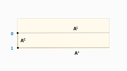
For the moment we will consider as a complex variable. In the complex -plane, the Pöschl-Teller potential possesses some symmetries. On the one hand it is symmetric with respect to shifts of in the imaginary direction. These give rise to an action of on the complex plane. In addition, the potential is also reflection symmetric, i.e. it is invariant under the reflection . Together, these two transformations generate the symmetry group of the Pöschl-Teller potential. The fundamental domain
for the action of in the complex -plane is shown in Figure 1. After the appropriate identifications of boundary points it has the form of a semi-infinite pillow, i.e. a semi-infinite cylinder whose end is squashed to an interval. The two corners of this semi-infinite pillow correspond to the two points and at which the Pöschl-Teller potential diverges. At the same time, these points are fixed under the action of a non-trivial subgroup of the symmetry on the complex -plane.111When , the fundamental domain is further reduced to . In this case, the complex torus has non-trivial (so called) center [44], which is related to existence of a minuscule weight for the reduced root system . The denominator is called an extended affine Weyl group, and the additional accounts for a permutation of an affine and a non-affine simple root. The reduced fundamental domain has , instead of . When , there is a remnant of this symmetry which we call , see below.
The group exhausts all the symmetries of the Pöschl-Teller potential that are associated with a transformation of the variable alone. But there exists one additional symmetry that involves a shift in combined with a reflection of the coupling .222This symmetry is a twist of an ordinary translation symmetry of the Pöschl-Teller problem, where is acts on coordinates only since the parameter vanishes. It may be regarded as a translation of the coordinate by a times a minuscule coweight of the root system , see below. More precisely, it acts as
| (2.2) |
while leaving the couplings invariant, i.e. . In fact, the Pöschl-Teller potential is invariant under these replacements
Note that the symmetry maps the two singular points and in the fundamental domain onto each other.
After these comments on the symmetries of the Pöschl-Teller potential let us now discuss the possible setups for the Schrödinger problem. These correspond to different 1-dimensional subsets on which the Pöschl-Teller potential is real. There are essentially three such choices which we shall denote by and . We define the set as
| (2.3) |
For this set, the Schrödinger equation reads
| (2.4) |
Note that the potential creates a wall at which shields the positive half-line from the negative one. In this case, there is a continuum of states with energy . We will discuss these in the next section. A second possible choice is
| (2.5) |
On this set, the corresponding Schrödinger equation is the same as on , except that the parameter is sent to . Our previous comments on the structure of the spectrum apply to this case as well.
There exists a qualitatively quite different choice for a domain on which the Calogero-Sutherland Hamiltonian is real. It is given by
| (2.6) |
where the superscript stands for compact. On the Schrödinger equation takes the form
| (2.7) |
Once again, there are infinite walls at . This setup describes a particle in a 1-dimensional box with infinitely high walls on both sides. In this case the spectrum is discrete. We will recall the precise form of the wave functions in the next section.
2.2 The Calogero-Sutherland potential
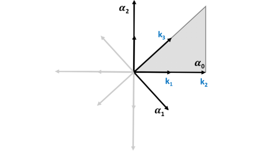
Before we can spell out the Calogero-Sutherland Hamiltonian, we need a bit of notation. In general integrable Calogero-Sutherland Hamiltonians are associated with a root system . Here we shall focus on BCN root systems, see Figure 2, whose positive roots are given
| (2.8) |
We have used to denote a basis of that is orthonormal with respect to the canonical scalar product . Note that this root system is not reduced, i.e. it contains roots that are related by a factor of two.333The integrality condition in the definition of a root system demands that a projection of a root onto any other root is a half-integer multiple of the latter. One can easily see that this can indeed happen if some roots possess a collinear partner differing by a factor of two, but not more. From time to time we will have to remove the shortest positive roots, i.e. the roots . The remaining set of positive roots is denoted by . Of course, are simply the positive roots of the Lie algebra . Let us also select a basis of consisting of
for . Indeed, all elements of may be obtained as linear combinations of with non-negative integer coefficients. The unique highest root is given by . For any root , we define
This concludes our short description of the root system and the special roots that will play an important role below.
The potential of the associated Calogero-Sutherland model takes the form
| (2.9) |
It involves the parameters , often referred to as multiplicities, that are assumed to be invariant under the action of the Weyl group of , i.e. for . Since the BC root lattice decomposes into three orbits under the action of the Weyl group, see Figure 2, the potential contains three independent parameters, which we parametrize as
| (2.10) |
in terms of the three parameters and . The reason for this choice of parameters will become clear in the fourth section. In addition, we agree that if . Finally, we have also introduced . It is easy to see that the formula (2.9) reduces to the Pöschl-Teller potential upon setting . Note that the root system for BC1 consists of two orbits under the action of the Weyl group . Hence, the potential only contains two parameters, and . Let us also note that the case is somewhat special since there are no contributions from the short roots in the potential. This means that the underlying root system is rather than BCN.
Example: The case we are most interested in appears for . The corresponding Calogero-Sutherland potential now contains all three parameters,
| (2.11) |
One may think of this potential as describing two Pöschl-Teller particles in the half-line that are interacting with an interaction strength depending on . Alternatively, one can think of a single particle that moves in an external potential on a 2-dimensional domain , see below.
2.3 Affine Weyl group and the domain
The analysis of symmetries of the Calogero-Sutherland potential proceeds pretty much in the same way as for the Pöschl-Teller problem. Once again, we will think of as complex variables so that the potential is a function on . Obviously, it is invariant under the independent discrete shifts
| (2.12) |
These generate the abelian group . In addition, the potential is also left invariant by the action of the Weyl group of the BCN root system. This Weyl group can be generated by the Weyl reflections that are associated with our basis . We shall denote these Weyl reflections by . It is not difficult to work out all relations among these generators. They are given by
| (2.13) |
for . All other pairs of generators simply commute with each other, i.e.
The Weyl group acts on the translations by permutation and inversion. More precisely one has the following set of non-trivial relations
| (2.14) |
for . Here we used a multiplicative notation for the generators of the abelian group , i.e. we denote the shift of by as rather than . Together, the elements and with generate the so-called affine Weyl group
| (2.15) |
The affine Weyl group describes all symmetries of the Calogero-Sutherland potential (2.9) that act on the coordinates alone. It generalizes the group we had introduced in our discussion of the Pöschl-Teller potential to the case with .
Here we have described the affine Weyl group in terms of generators and with . There exists a second description in terms of generators with . While with are the same Weyl reflections we used before, the new generator is given by
| (2.16) |
One may check by explicit computation that this new element satisfies the following relations with
| (2.17) |
for . Note that the relation between and is identical to the one between and . Obviously, one can reconstruct the generator from the element and the Weyl reflections . The other elements are then obtained by conjugation with .
As in the case of the Pöschl-Teller potential there exists one additional shift symmetry that requires a combined action on the coordinates and the coupling constants. It is given by
| (2.18) |
while leaving the other two couplings and invariant. Note that involves a simultaneous action on all coordinates. Following the same steps as in the section 2.1 one finds that
| (2.19) |
Let us stress that this symmetry is not part of the affine Weyl group which acts only on coordinates.444As in the Pöschl-Teller case, this symmetry is a twist of an ordinary translation symmetry of the Pöschl-Teller problem for which it acts on the coordinates only. The latter may be considered as a translation of by times a minuscule coweight of the reduced root system .
We are now well prepared to discuss the domain(s) on which we will consider the Calogero-Sutherland system. We start with a set of complex coordinates and implement the identification furnished by the the discrete shifts . This leaves us with an -dimensional complex manifold
The manifold contains an -dimensional real submanifold that is parametrized by , modulo identification with . We can shift with to obtain . The latter is parametrized by with real .
The Calogero-Sutherland potential diverges along the following walls of real codimension two
that are in one-to-one correspondence with the positive roots of our BCN roots system. Note that for the long roots , the set possesses two disconnected components, one of which coincides with the wall for the corresponding short root. The walls associated with the roots contain a single connected component. By construction, the walls are invariant under the action of the reflection .
The walls we have just described are subspaces along which the Calogero-Sutherland potential diverges so that the corresponding Schrödinger problem can be restricted to various subsets within the quotient space
| (2.20) |
which describes a fundamental domain555As in the Pöschl-Teller case, when the fundamental domain becomes . Again, the root system becomes of reduced, type. The denominator is an extended affine Weyl group. The nontrivial element in the additional accounts for a permutation of an affine and a non-affine simple root that preserves the Weyl alcove. When , there is a remnant of this symmetry which we again call . for the action of the Weyl group on . Representatives of the quotient space in intersect with only walls where for and are the two disconnected components of with .
Once again, the fundamental domain for the Calogero-Sutherland problem possesses several subsets along which the the potential is real. The most important is the Weyl chamber
| (2.21) |
In this case, the eigenfunctions possess continuous variables. As in the case of the Pöschl-Teller problem, we can also consider the shifted Weyl chamber . It gives rise to a similar set of wave functions except that the coupling must be replaced by . Another extreme possibility is the case
| (2.22) |
for which the spectrum of the Calogero-Sutherland model is discrete. But in the multivariable case there are many other possibilities. We will discuss a few of them for .
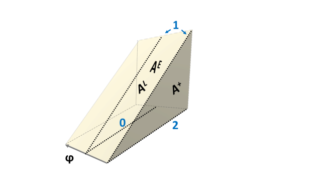
Example: Let us give some additional details for . In this case, the Weyl group consists of eight elements. It can be generated from and subject to the relations
| (2.23) |
The fundamental domain for the action of the Weyl group on , or rather a 3-dimensional subspace thereof that satisfies , is shown in Figure 3.
Once again, we can consider the Schrödinger equation for the Calogero-Sutherland potential on various real subsets . The most standard choice in the mathematical literature is
| (2.24) |
This is simply a Weyl chamber for the BC2 root system. As for the Calogero-Sutherland potential diverges along the walls of the chamber, see our discussion above.
There are two additional choices we want to discuss here because of their relevance for conformal field theory, see section 4 below. The first one is given by
| (2.25) |
It may be obtained from by application of combined with a translation by . The associated Schrödinger problem has the same form as on , except that the parameters are changed, see our discussion above
| (2.26) |
Another relevant possible subset that leads to real potential is the one in which the two coordinates and are complex conjugates of each other,
We shall decompose into its real and imaginary part. In this case we are dealing with a particle that moves on a 2-dimensional semi-infinite strip given by and . For large the potential becomes
So, we see that in this asymptotic regime, wave functions are given by a product of a Pöschl-Teller bound state and a plane wave in the -direction.
2.4 Coordinates in the CS problem
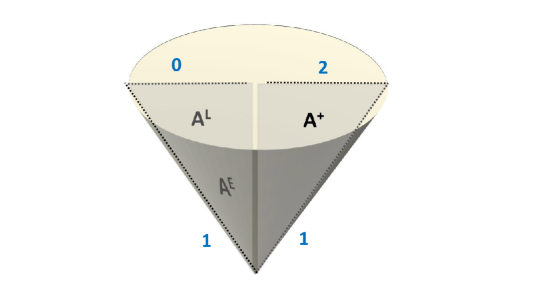
Let us conclude this section with a short comment on coordinates. So far, we have described the Calogero-Sutherland problem in terms of coordinates in which the kinetic term is simply the standard flat space Laplacian. Since the are coordinates on it is tempting to apply the exponential map that sends to .666To be more precise, this map is injective, with the image , and thus defines a partial compactification of the complex torus. By the action of the Weyl group, it extends to a toroidal compactification of the torus corresponding to its decomposition into Weyl chambers. This gives the toric variety of -coordinates, see [57] (page 55), [58, 59] for details. Indeed, we shall often use the coordinates
| (2.27) |
instead of . This has the advantage that the identification is manifest. Upon application of the exponential map (and inversion), the 3-dimensional slice of the fundamental domain that is shown in Figure 3 gets mapped to a cone, see Figure 4. The map sends the Weyl chamber and the space to one half of a section through the cone each, while the set becomes half of the mantle of the cone. Figure 4 also keeps track of the location of the singularities.
While the coordinates make the identification with manifest so that they are proper coordinates on , the identification from the action of the Weyl group is not built into these coordinates. It is often good to do a little better and to use coordinates that are invariant at least under the action of the Weyl reflections . Any function of would do the job, but we shall adopt a very specific one, namely 777A bit more precisely, for we will use the branches in order to be consistent with definition (2.25).
| (2.28) |
These coordinates send the domain to configurations that are symmetric under the action of the permutation group . The latter is generated by the Weyl reflections for .
3 Wave functions of the Calogero-Sutherland model
Having set up the eigenvalue equation we want to study we now turn to a discussion of the solutions. As a warmup, we briefly look at the example of the Pöschl-Teller problem for which the study of wave functions involves some fairly basic facts from the theory of Gauss’ hypergeometric functions. Then we turn to general and discuss a basis of scattering states that are known as Harish-Chandra functions. We will discuss their definition and a new series expansion formula for along with a few direct consequences. As a main application, in the third subsection we provide a complete analysis of poles and residues of Harish Chandra functions for . The fourth subsection finally, is devoted to the construction of physical wave functions. Through a general discussion of the monodromy representation for the Calogero-Sutherland eigenvalue problem we are led to consider special linear combinations of Harish-Chandra functions that possess good analytic properties along the walls of the scattering problem. The optimal choice corresponds to the so-called Heckman-Opdam multivariable hypergeometric functions and, for , a Euclidean analogue thereof.
3.1 Wave functions of the Pöschl-Teller problem
Here we will mostly study the Pöschl-Teller Hamiltonian on the domain that was introduced in the previous section. The corresponding eigenvalue equation was stated in eq. (2.4). We shall make the following Ansatz for the wave function
| (3.1) |
As before, denotes the parameters of the Pöschl-Teller potential and is the momentum. In our conventions it is related to the energy eigenvalue in eq. (3.1) through so that is purely imaginary for positive energy solutions.
Since the Pöschl-Teller potential tends to zero at , the eigenfunctions of the Pöschl-Teller Hamiltonian are superpositions of an outgoing and an incoming plane wave in this asymptotic regime. We can choose a basis for which one of the two wave functions of energy is purely outgoing while the other is purely incoming, i.e.
| (3.2) |
Wave functions with these asymptotic properties are also referred to as Harish-Chandra functions. These two wave functions with eigenvalue can easily be constructed in terms of Gauss’ hypergeometric functions as888Here and in the following, we choose the principal branch for and insist on in the -plane.
| (3.3) |
where and are related through equation (2.28). For large values of , the argument of the hypergeometric functions approaches zero and the asymptotics of the prefactor combine with that of the gauge transformation to give the desired asymptotics (3.2). Since the standard series expansion for converges on the real -line for and our parameter takes values on , the usual series expansion of the function (3.3) converges in the entire Weyl chamber.
In the context of Calogero-Sutherland models, one usually requires the series expansions in the variable to be convergent throughout the Weyl chamber, see below. We shall refer to such expansions as -expansions, even though they are really expansions in . To obtain such a -expansion for the case at hand, one simply expresses through in the series expansion of (3.3)999To avoid additional subtleties, we keep the momenta generic here, namely we assume that . Special cases can be obtained by carefully taking limits, see comments in section 3 and appendix B. and then expands in powers of . This second expansion is absolutely convergent for . We arrive at
| (3.4) |
In accord with the general analysis (see next subsection), this expansion is convergent on the entire domain . It can be analytically continued to the strip , which is a tube-like neighborhood of . If in (3.4), one can use Watson’s summation for [60] to sum the -expansion formula (3.4) into
The resulting expression is well known from the theory of Calogero-Sutherland wave functions for the reduced root system .
After this short detour on series expansions for the in- and outgoing wave functions we come back to the problem of constructing physical wave functions for the Pöschl-Teller problem. Clearly, the two wave functions we considered so far are badly behaved when we approach the wall at . In fact, is a branch point. But there exists a unique linear combination of these two wave functions that is analytic at . It is given by
| (3.5) | |||||
with coefficients given by
These values then allow to apply Kummer’s identity in order to pass from the first to the second line in eq. (3.5). Obviously, the branch point at , or equivalently at , has been removed now. After multiplication with the factor , gives what we would usually consider the physical solution of the hyperbolic Pöschl-Teller system. The eigenfunctions with form a complete orthonormal basis of eigenfunctions for the hyperbolic Pöschl-Teller problem on [61], with (appropriately normalized) measure .
The branch points of at prevent us from continuing the purely in- and outgoing wave functions beyond into the compact domain that was defined in eq. (2.6). On the other hand, the function can be continued into . For generic choices of the resulting wave function of the trigonometric Pöschl-Teller problem (2.7) possesses a branch point at . This branch point can only be avoided for a discrete set of . In this way one obtains the usual eigenfunctions of the trigonometric Pöschl-Teller problem
| (3.6) |
for where the variable is restricted to the interval so that it parametrizes . Note that for , i.e. for the ground state, the hypergeometric function contributes a trivial factor. Hence, the wave function of the ground state in the compact domain coincides with the function we introduced in eq. (3.1).
Let us finally also discuss the wave functions of the Pöschl-Teller problem on the shifted domain that we defined in eq. (2.5). In this case, we select the Harish-Chandra functions such that the eigenfunctions possess the standard asymptotics in the real coordinate on , i.e.
| (3.7) |
Of course this implies that the Harish-Chandra functions are related to by a -dependent gauge transformation
| (3.8) |
Solutions of our Calogero-Sutherland problem with these asymptotics take the form
| (3.9) |
The relation (3.8) with the standard Harish-Chandra functions is then a consequence of the Pfaff transformation for Gauss hypergeometric function [60]. In writing our formula for we agree to use the principal branch for so that in -plane the twisted Harish-Chandra function has cuts along for generic values of parameters. Note that on the variable takes values in , so that this usual series expansion of the functions is convergent on the entire shifted Weyl chamber. As above, this function can be analytically continued to a semistrip . Once again we need to form a special linear combination of these twisted Harish-Chandra functions to obtain the physical wave function which is regular at or equivalently . It is given by
| (3.10) | |||||
with coefficients
We observe that can be obtained from through the inversion of the parameter . This replacement agrees with the action of the shift on the coupling constants in the Pöschl-Teller problem, see eq. (2.2). The functions for provide us with a complete orthonormal basis of eigenfunctions for the Pöschl-Teller problem on .
There is a different, more algebraic way to express these results on the construction of physical wave functions for the Calogero-Sutherland problems through representations of the fundamental group . Recall from the previous section, that the domain is a semi-infinite pillow. Hence, its fundamental group is freely generated by two elements and . These are described by loops around the singular points and . The Harish-Chandra functions carry a 2-dimensional monodromy representation of this fundamental group. We can easily infer the representation matrices from standard properties of hypergeometric functions, along the lines of our discussion above. For one finds that
| (3.11) |
where the matrix is given by
and is obtained by reversing the sign of both and . Our discussion of the regular solution at shows that can be computed in the same way after we perform a gauge transformation from to , i.e.
| (3.12) |
where is obtained from by the substitution and the matrix encodes the gauge transformation (3.8). It reads
We observe that both monodromy matrices possess one eigenvector with unit eigenvalue. This signals the existence of a special linear combination of Harish-Chandra functions which has trivial monodromy around and , respectively. Explicitly, these eigenvectors were given by the functions and . Finally, we also want to stress that the product of the two monodromies describes the monodromy of the Harish-Chandra functions at . The latter is fully determined by asymptotic behavior of Harish-Chandra functions, i.e.
| (3.13) |
We will now explain that all this carries over to . In particular, the monodromy group and its representation on Harish-Chandra functions is explicitly known, see the section 3.4 below.
3.2 Harish-Chandra series expansions
Let us now discuss eigenstates of the hyperbolic Calogero-Sutherland Hamiltonian for . Our discussion will start with the Weyl chamber in which all the are real and positive. To construct the solutions we are interested in, we note that in the region of large where we are far away from all walls of the Weyl chamber, the Calogero-Sutherland potential goes to zero and hence, in this regime, any wave function is a superposition of plane waves. Before we give precise definitions let us split off a simple factor from the eigenfunctions and introduce a new function through
| (3.14) |
The factor is split off for convenience, see below. In the case of it reduces to the one we worked with in the previous subsection in order to map the eigenvalue equation for the Pöschl-Teller Hamiltonian to the hypergeometric differential equation in the variable . We will often refer to the factor as a gauge transformation and to as a Calogero-Sutherland wave functions in hypergeometric gauge. Let us note in passing that the function possesses the following asymptotics for large ,
| (3.15) |
So-called Harish-Chandra wave functions are symmetric solutions of the Calogero-Sutherland Hamiltonian for which possesses the following simple asymptotic behavior
| (3.16) |
where is the vector of momenta and in means that all components become large while preserving the order . Recall that symmetry means that depends on the through and that it is symmetric under all permutations of the . The condition (3.16) selects a unique solution of the scattering problem describing a single plane wave. It is analytic in the Weyl chamber . The corresponding eigenvalue of the Calogero-Sutherland Hamiltonian is given by
When we required the Harish-Chandra functions to be symmetric, we used the action of the Weyl group on the coordinate space . On the other hand, the Weyl group also acts in a natural way on the asymptotic data of the Harish-Chandra functions by sending any choice of through a sequence of Weyl reflections to . Since the eigenvalue is invariant under all the reflections, our Harish-Chandra functions come in families. For generic choices of , one obtains solutions which all possess the same eigenvalue of the Hamiltonian.
At least for sufficiently generic values of the momenta,101010A precise formulation of the condition is given below through the inequalities (3.19) and the subsequent discussion. Harish-Chandra functions can be constructed as a series expansion in the variables
| (3.17) |
where we adopt for on the principal branch of BCN Harish-Chandra functions and we sum over elements of the -cone over the positive roots, i.e. the set
For later discussions we note that comes equipped with a partial order where iff .
It is not difficult to derive recursion relations of the expansion coefficients directly from the Calogero-Sutherland eigenvalue problem, see e.g. [57] 111111The recursion derived in [62] is closely related to this one, specialized for . However, our expansion here is in monomials, not in Gegenbauer polynomials, although it is not difficult to go between the two.
| (3.18) |
This can be solved uniquely, if
| (3.19) |
The resulting series are known to converge121212The series converges absolutely and uniformly on compacta in the set of complexified momenta and multiplicities times , as long as they are chosen to avoid the hyperplanes (3.19). within the Weyl chamber [57], as is fairly obvious from the physics they describe. Even when one of the conditions (3.19) is violated it is possible to obtain a complete basis of series solutions . There is a subset of such cases where things are a bit subtle, namely when is chosen such that is integer which implies that one of the conditions in eq. (3.19) is violated. For such values of non-generic momenta some of the series solutions are logarithmic. This is analogous to usual properties of the Gauss hypergeometric function when the difference of exponents becomes integer [60]. To obtain their expansions, one needs to see which fundamental solutions coincide on the corresponding locus and take the limit of their rescaled difference as a new fundamental solution.
Example: Let us look at the Harish-Chandra functions for in some detail. Although, we could literally repeat the entire discussion here, we leave much of it for appendix A.131313In appendix A, we derive a -expansion for twisted Harish-Chandra function which is related to the present one by formula (3.52). In particular, this appendix contains explicit expressions for the expansion coefficients in the -expansion (3.17), see eq. (A). We do not want to repeat these here and will rather discuss a somewhat intermediate form of a -expansion from which we shall derive many interesting properties properties of Harish-Chandra functions in the remainder of this and in the next subsection. It is given by
| (3.20) | ||||
As in the discussion for we choose the principal branch for , so that . It is obvious that this function has the correct asymptotic behaviour. Let us stress that, unlike a somewhat similar expansion for conformal blocks that appears in [25], our expansion for Harish-Chandra functions is also valid for non-integer spins . We can use it to derive a corresponding expansion for conformal blocks once we have explained how to construct blocks from Harish-Chandra functions in the next section. The derivation of eq. (3.2), its features and equivalent expansions are described in appendix A. We note that the -expansion (3.2) is convergent for arguments in the region
| (3.21) |
which includes the entire Weyl chamber, similarly to the case. Here we assume that the parameters are generic.
As an immediate application of the series expansion (3.2) we can evaluate Harish-Chandra functions for some special values of the multiplicities . For , for example, the multiplicity vanishes so that one of the upper parameters in the balanced inside the sum coincides with one of the lower ones. The sum involving the resulting balanced is summable via Saalschütz identity [63] and we obtain
The result is a product of Harish-Chandra functions for the Pöschl-Teller problem , see eq. (3.3). The case of is even simpler to evaluate. Indeed, for this value of , the parameter and hence one of the upper parameters in the balanced tends to zero, so that we obtain
Before we derive further properties of Harish-Chandra functions for from the series expansion (3.2), we want to review a few more general properties that hold for any .
The last two formulas for that we derived from the -expansion (3.2) possess a nice generalization to arbitrary values of . For and generic (non-resonant) values of the eigenvalues is known that [64]
where
is a Weyl denominator for middle roots. More generally, it is known [65, 64] that Harish-Chandra functions for any positive integer value of the multiplicity are multilinear combinations of Pöschl-Teller wave functions. The most elegant derivation of such expressions, one that is also completely universal in , involves differential or difference operators which shift by one unit. For scalar 4-point blocks similar constructions are known from the work of Dolan-Osborn [25, 26]. We will show how explicit closed formulas for these operators follow from the integrable structure of Calogero-Sutherland models in a forthcoming publication [50].
3.3 Poles and residues of Harish-Chandra functions
Our short excursion to explicit expressions for Harish-Chandra functions which exist for special values of the multiplicities only should not mislead the reader to think that Harish-Chandra functions can only be understood for very special cases. In fact, it is one of the central virtues of Heckman-Opdam theory that one is able to say so much about Harish-Chandra functions often without knowing their explicit series expansions or integral formulas. As an example for one of the many further properties that is well understood beyond the simple case of let us mention that are entire functions of the multiplicities and meromorphic function of asymptotic data , for any choice of in the fundamental domain. They are known to possess simple poles whenever the set of satisfies one of the following conditions
| (3.22) |
Let us note that given satisfying this condition, this violates the condition (3.19). In fact, the quadratic expression in eq. (3.19) vanishes at least for . The converse is not true, i.e. there exist many values of that violate the inequalities (3.19) but do satisfy the condition (3.22). At such values of Heckman and Opdam showed that the singularities are only apparent. For the true poles at , the residues are given by (see e.g. [65])
| (3.23) |
where indicates that the relation with the Harish-Chandra function holds only up to an constant factor. The latter is not known in general, but we shall explain later how it can be determined and provide explicit expressions for with the help of the series expansion (3.2).
Relation (3.23) is actually a little more subtle than it may appear at first. According to a theorem by Heckman ([57], Cor. 4.2.4), eq. (3.23) holds true as it stands whenever the quadratic equation has exactly one non-zero solution . In this case, one has
| (3.24) |
Here, the Harish-Chandra function on the right hand side appears from summing over all terms in the original series with with respect to the partial ordering of we introduced above. If the quadratic equation has several solutions in , on the other hand, relation (3.23) holds only for a properly defined Harish-Chandra series on the right hand side. One can do this by approaching the desired limit point along a sequence of irrational values for which has a unique solution. Then, provided one knows the series expansion of Harish-Chandra function for such , it is possible to calculate its residues by Heckman’s theorem.
Example: Let us continue our tradition to describe a few more details in the case of . As we discussed before, the corresponding Weyl group is eight dimensional. It is generated by the two reflections and . All eight elements are listed in table 1 along with their action on the asymptotic data of the Harish-Chandra functions. In the case at hand, the shift by reads
The final column of table 1 will be explained in section 4. It describes the asymptotic data in a different parametrization.
If we denote an element of as for , the locally finite set of hyperplanes on which the definition of the Harish-Chandra series requires an appropriate limiting procedure reads
| (3.25) |
As we stated before, only a small subset of these hyperplanes give actual poles. Namely, according to equation (3.22) the Harish-Chandra functions possess four series of poles in the asymptotic data . In fact, while the set of positive roots contains six elements, the solutions of eq. (3.22) for the longest roots form a subspace of the solutions for the short roots . The relevant four roots are listed table 2 along with the corresponding Weyl reflection written in terms of our fundamental generators and . For each of these four cases, the solutions of eq. (3.22) are listed in the third column. They depend on a non-negative integer and one free parameter . The residues of our Harish-Chandra functions for these values of are again given by Harish-Chandra functions with different asymptotic data. The latter is listed in the forth column of table 2. The information of the third and forth column is repeated in the last two columns in a different parametrization of the asymptotic data that we explain in section 4.
In order to obtain exact formulas for the residues, including the numerical coefficients, we shall employ the series expansion (3.2). The general idea is simple to state. As we know, the residue should be proportional to a Weyl-reflected Harish-Chandra function, so one just needs to locate the terms of the series expansion that diverge as we send close to a corresponding pole position. Within the set of these divergent terms one needs to identify the one that gives the leading power of and read off the coefficient. Heckman’s theorem quoted above guarantees that we can interchange the summation and the limit. In principle, the described steps can be carried out both for the usual -expansion (see appendix A) and the -expansion we spelled out in equation (3.2). Here we shall sketch the derivation from the latter and spell out the explicit residues for all four families of poles.
According to our table, the residue for the series is proportional to . It is easy to see that the leading divergent term in the -expansion (3.2) arises from the summands with , , . Here and in the following, the summation index refers to the series expansion of the hypergeometric function in the last line of equation (3.2). Hence, the two hypergeometric functions in the summands of eq. (3.2) can be replaced by in all divergent terms. Keeping in mind that , we obtain
so that the residues are given by
| (3.26) | ||||
The evaluation of the residue for the family is even simpler. Since it is proportional to , it must arise from the terms , , in eq. (3.2). Once again it is easily seen that the two inner hypergeometric functions that appear in the summands do not contribute so that the residue reads
| (3.27) |
For the third family of poles at the residue is proportional to . The relevant terms in the sum arise from , . For these values of indices, the inner still does not contribute, but the does, as none of the upper parameters is zero anymore. Furthermore, in the present case the Pochhammer symbol that produces the desired pole is among the lower ones in the series expansion of the inner function. To take it out, we use a Whipple transformation for balanced [63]
Substituting , taking and expanding the balanced on the right hand side of the last formula in , we see that its leading term is not singular now. Moreover, one upper and one lower parameter in it cancel against each other and we are left with a balanced function that can be summed by a usual Saalschütz formula [63]:
where the dots denote subleading orders in . All in all, the residue is thus again given just by a product of Pochhammer symbols
| (3.28) | ||||
The last sequence of poles at with residues proportional to , is again simple. In this case the leading terms arise from to , , so the inner does not contribute, whereas the does. Therefore, we readily obtain
| (3.29) |
Notice that all the residues are symmetric under , , as they should be in consistency with the symmetries of Harish-Chandra function described above. Let us also note that, for generic multiplicities and eigenvalues , all four families contribute an infinite sequences of poles.
3.4 Monodromy group and representation
As in the case of the Pöschl-Teller problem, imposing good features of the wave functions at the walls of requires to consider certain linear combinations of Harish-Chandra functions. For the BCN Calogero-Sutherland model, the Weyl chamber possesses walls which are in one-to-one correspondence to the generators of the Weyl group. As we have discussed above, there is one more wall , but it does not bound the domain and so is not of concern for us, at least for most of this section. Since there are Harish-Chandra functions and hence coefficients to fix in their linear combinations, one might naively expect that analyticity at the walls would leave some coefficients undetermined. It turns out, however, that there exists a unique linear combination (up to a constant factor) that is analytic at all walls on the boundary of the Weyl chamber.
The prescription to build such analytic wave functions is not difficult to state. Suppose we want the wave function to be analytic at some subset consisting of of the walls that bound , i.e . To each of these walls there is a generator of the Weyl group and so our set of walls is associated with a subgroup of the Weyl group that is generated by . Given this subgroup we now define the following superposition of Harish-Chandra functions
| (3.30) |
where the so-called Harish-Chandra c-function141414This function is an analytic continuation of the so-called Gindikin-Karpelevic c-functions [66] in harmonic analysis. reads
| (3.32) | |||||
Any wave function of this form turns out be be regular at the walls . There are two extreme cases of this construction. If we just demand regularity at a single wall , then the subgroup consists of two elements, the identity and the reflection . Hence, from the orbit of Harish-Chandra functions we obtain linear combinations that are regular at . If, on the other hand, we want a wave function that is regular at all the walls that bound , then the subgroup coincides with the Weyl group and we end up with a unique linear combination. Let us note that while this function is analytic in a neighborhood of , it fails to be analytic at the wall . The function is also known as Heckman-Opdam hypergeometric function. More generally, linear combinations of the form (3.30) are referred to -hypergeometric functions, see e.g. [67] and references therein.
One can also build a function that is analytic at , but has monodromy around . We will give an exact formula in the case of below. The corresponding wave functions and with are the physical wave functions of the Calogero-Sutherland problem on and , respectively. Hence, they provide an orthogonal basis within the space of functions on the and .[57, 68, 65] In hypergeometric gauge the Hermitian scalar product on reads151515This formula defines an inner product only if certain conditions on the multiplicities are satisfied, e.g. if for all .
| (3.33) |
where is a suitably normalized measure on [68]. The gauge transformed Calogero-Sutherland Hamiltonian is self-adjoint with respect to this inner product.
As in the case of there exists a nice reformulation in terms of the representation theory of the fundamental group . The latter is generated by elements which are associated with closed loops around the walls of the Calogero-Sutherland potential [69, 57] (see also [70]). Note that the real codimension of these walls in complex space is two. Since the walls are associated with generators of the affine Weyl group , so are the generators . One may show [69] that the generators of the fundamental group satisfy the following set of relations
| (3.34) | |||||
| (3.35) | |||||
| , | (3.36) |
These are very similar to the defining relations of the affine Weyl group, except that in the fundamental group . So, the relation between the monodromy group of and the affine Weyl group mimics the relation between the braid group and the permutation group. Therefore, the fundamental group is also referred to as (Artin) affine braid group. Note that the relation in the second row is the usual braid or Yang-Baxter equation. The relations in the third line, which involve the elements and , on the other hand, resemble forth order reflection equations in which two factors on each side arise from the reflection at a boundary while the other two are associated with scattering in the bulk.
For the affine Weyl group we actually discussed two different presentations, one in terms of generators and a second one that involves generators and with . In complete analogy to the construction of the generators , we can build [71, 72, 57] (see also [73]) a set of commuting generators through
| (3.37) |
The reader is invited to verify that . Hence the group elements generate an -dimensional lattice . The generators act on this lattice as
| (3.38) | |||||
| (3.39) |
Our conventions on directions of the basic loops match [57] (section 4.3) if we identify our generators with the generators used by Heckman as .
For generic values of , the space of Harish-Chandra wave functions forms a -dimensional representation of the monodromy group . This representation is explicitly known due to the work of Heckman and Opdam. With respect to the action of , the space of Harish-Chandra functions splits into 2-dimensional subspaces each of which is spanned by a pair of Harish-Chandra functions and . On these subspaces, the action is given by
| (3.42) | |||||
| (3.45) |
The matrices are defined as
where denotes an involution of the multiplicities (see also below) and
| (3.46) | |||||
| (3.47) |
is the same function that appeared in our discussion of the Pöschl-Teller problem. The monodromy representation of the element is once again obtained from by the simple replacement along with a gauge transformation of the form
where is the sum of short roots.161616The mathematical origin of this is that it is twice the minuscule co-weight of root system . In this way, it is related to a symmetry that interchanges the -th and -th affine root, see previous discussion. So, in formulas one has
| (3.48) |
Here denotes the matrix in eq. (3.45) with replaced by . Note that the monodromy matrices for the curves around the walls do not depend on and are left invariant by the gauge transformation, i.e. . One may check that the monodromy matrices satisfy all the defining relations of the fundamental group . In addition they possess the following Hecke property
| (3.49) | |||||
for and . The Hecke property of the monodromy matrix is obvious from the eqs. (3.42), (3.45) and (3.48). The formulas for the monodromy representation we have displayed here imply that the functions we defined above indeed have trivial monodromy with respect to .
One might wonder why these formulas are so similar to the ones in the Pöschl-Teller problem. The reason is however not so difficult to grasp. If we start our curve near asymptotic infinity we can reach each of the walls separately, i.e. we can move near any of the wall while staying far away from the others . In this way, the monodromy problem for a given wall can really be solved within the theory of single variable hypergeometric functions. The walls and are in fact entirely equivalent to the walls in the Pöschl-Teller problem while the intermediate ones possess a different dependence on the coupling constants. The latter may be understood through a replacement and in the expression for .
We have also promised some more comments on the origin of the multiplicities that occur in the second row of the matrices. These may be traced back to symmetries of the Harish-Chandra functions. Indeed, it is well known that [74]
| (3.50) |
and denotes the set of middle and long positive roots, i.e. in the product that defines we do not include factors for the short roots. In terms of our parameters the involution reads .
Before we return to our discussion of the special case of , we want to conclude the general discussion on the monodromy representation of the affine braid group by stating a general result from [57] (proposition 4.3.10) that provides a criterion for the irreducibility of the -dimensional representation in the space of Harish-Chandra functions. According to this theory, the representation we have described is irreducible, provided that the momenta and the multiplicities are sufficiently generic, i.e. that
| (3.51) |
for all roots of the root system. When one of these conditions is violated, the monodromy representation may contain non-trivial subrepresentations. We will see one such example below.
Example: Let us discuss some more details for the case of that is most relevant in the context of conformal field theory. We have noted already that the corresponding Weyl group possesses elements. The eight Harish-Chandra functions give rise to an eight-dimensional monodromy representation of the fundamental group . The latter is generated by three elements subject to the following relations
These are associated with the three walls in Figure 3. Among the linear combinations of Harish-Chandra functions, there are a few that we would like to highlight. The first one is associated with the subgroup that is generated by . According to the general theorem we quoted above, the following symmetric combination of Harish-Chandra functions
is regular at the wall , see Figure 3. Note that acts on momenta of Harish-Chandra functions by exchanging and . The functions coincide with the functions with we introduced above up to a constant (-independent) factor. Since is analytic at the wall , it can be continued from to and further into . On the other hand it fails to be analytic at the walls and . In order to obtain a regular wave function at the wall and hence in a neighborhood of the domain , we must add a whole 8-dimensional orbit of Harish-Chandra functions under the action of the Weyl group on the asymptotic data . The coefficients are given by the Harish-Chandra c-function that we defined in eq. (3.32).
If instead we want a wave function that is regular at the walls and and hence in a neighborhood of we must sum the twisted Harish-Chandra functions171717We assume , here.
| (3.52) | ||||
| (3.53) |
over an entire orbit of the Weyl group with coefficients given by a twisted version of the Harish-Chandra c-functions (3.32) ( i.e. in which is replaced by ). Since the element of the Weyl group does not commute with the gauge transformation , the resulting function is not a constant multiple of . By construction, the Heckman-Opdam hypergeometric functions and trivialize two monodromies each, e.g.
and similarly for but with instead of . This concludes our discussion of wave functions on and the Lorentzian domain .
The hypergeometric functions we constructed in the previous example provide physical wave functions for the domain and the Lorentzian domain , respectively. Their construction is well known in the mathematical literature. For our purposes below we are also interested in the physical wave functions for the Euclidean domain . As far as we know, there exists no general theory for these functions, but for the specific example of such wave functions have been discussed in the context of conformal field theory [75, 51]. The former paper also contains a partial characterization in terms of monodromies. Recall that the Euclidean domain is bounded by the wall . To be slightly more precise, the strip is bounded by two semi-infinite lines satisfying (up to shifts by ) which arise from the wall and a compact interval along that is associated with the image of the wall under the Weyl reflection with . Consequently, one can characterize the physical wave functions for the Euclidean strip through the following three monodromy conditions
| (3.54) | |||||
It is easy to see that these three conditions cannot be solved simultaneously unless the is a non-negative integer. From now on until the end of this section we will assume that the parameter is generic, i.e. is not an integer. In this case, the unique (up to normalization) solution is given by
| (3.55) |
with
where is the conventional shorthand for and denotes a matrix element of the monodromy matrix (3.45) for . While the first two monodromy conditions in the list (3.54) possess four linearly independent solutions, the third condition puts the wave function on the semi-infinite strip and hence imposes strong additional constraints. As in our discussion of the theory, regular wave functions can only exist for a discrete set of values . Since the strip is infinitely extended in one direction, the sum can assume any imaginary value. When becomes infinite, the wave functions factorize into a product of Poeschl-Teller wave function of the form (3.6)181818With parameters replaced by and to account for the strength of the potential at the wall . and a plane wave in the coordinate . The latter possesses an incoming and an outgoing component.
Let us conclude this discussion of the Euclidean domain with a few general observations concerning the structure of the monodromy representations that occur when we specialize the spin to be integer. As we will argue now, the corresponding eight-dimensional representations of the affine braid group are indecomposable but no longer irreducible, i.e. they contain a non-trivial invariant subspace which turns out to be four-dimensional. This is consistent with the criterion (3.51). In fact, for it states
which is violated for the representations we are considering. It is indeed easy to see that the four Harish-Chandra functions
span a four-dimensional subrepresentation. In fact, while the first two functions are invariant under the action of , the remaining ones are just mapped onto each other. The monodromy matrix , on the other hand, mixes the first and the third function and similarly the second and the fourth. All four functions are eigenfunctions of the generators and hence no element within the affine braid group can ever get us out of the space spanned by these four functions. On the other hand, the remaining four Harish-Chandra functions from the eight-dimensional monodromy representation do not span an invariant subspace, i.e. the monodromy representations are indecomposable when is integer. Let us also note that the wave function we constructed above, is contained in the four-dimensional invariant subspace.
4 Wave functions and conformal blocks
After this lightning review of Heckman and Opdam’s work on the Calogero-Sutherland problem we want to explain how all this is related to the theory of conformal blocks for four external scalar fields. We shall begin with a brief reminder on the Casimir equation for conformal blocks before we explain the relation in the case of the theory that applies to 4-point blocks of bulk fields in 2-dimensional theories as well as to blocks of two scalar bulk fields in the presence of a boundary in any dimension [76]. Then we turn to conformal 4-point blocks in any dimension and their relation to the BC2 Calogero-Sutherland model, following [49]. In particular we will construct higher dimensional conformal blocks and their shadows in terms of the BC2 Harish-Chandra functions.
4.1 Conformal blocks and the Casimir equation
It is time now to embed the theory of scalar conformal blocks into the framework of the Calogero-Sutherland model that we have sketched in the previous two sections. To begin with, let us recall the precise definition of scalar conformal 4-point blocks as solutions of the so-called Casimir equation. [25] We consider the correlation function of four scalar conformal primary fields of weight in a -dimensional conformal field theory. Using conformal symmetry, this 4-point correlator can be written as
| (4.1) |
with and . The conformal invariants are introduced to parameterize the more familiar cross ratios as
| (4.2) |
For a Euclidean theory, are complex conjugates. When we work with Lorentzian signature, on the other hand, the variables and are real and taken from the interval . The function receives contributions from all the primary fields that can appear in the operator product expansion of the fields and
| (4.3) |
This expansion separates the dynamically determined coefficients of the operator product from the kinematic conformal blocks . The latter are eigenfunctions of the quadratic conformal Laplacian ,
| (4.4) |
with eigenvalues
| (4.5) |
The form of the conformal Laplacian has been worked out in [25],
| (4.6) |
where and
| (4.7) |
is defined similarly in terms of . In order to fully determine the conformal blocks, we impose the following boundary condition
| (4.8) |
when are close to and we choose the normalization factor to be
The condition (4.8) selects a unique solution of the conformal Casimir equation and therefore completes our definition of scalar 4-point blocks.191919Our normalization conventions match those of [26] (up to a change which is a symmetry of blocks). To match with [51], one should strip off the prefactor .
4.2 Blocks and the Pöschl-Teller problem
We can gain some first insight into the relation between conformal blocks and Harish-Chandra functions by setting . The conformal Casimir equation then decomposes into two independent equations that determine the dependence of blocks on and , respectively. Focusing on the -dependence leads to the following second order differential equation
Note that and hence the eigenfunctions depend on but we do not display this dependence explicitly. The same equation also appears for the blocks of two scalar fields in the presence of a boundary in -dimensional conformal field theory, see [76]. Following [49] we perform the gauge transformation
| (4.9) |
where the coordinates and are related through eq. (2.28) as before. Note that we consider the region in which which means that with
Inserting these relations it is easy to see that the function is an eigenfunction of the Pöschl-Teller Hamiltonian with potential where the coupling constants are the same as the parameters in the conformal Casimir equation, i.e. they are related to the holomorphic weights of the external fields through and . The eigenvalue , on the other hand, is determined by the holomorphic weight of the intermediate field . Hence we read off that .
If we compare the relation (4.9) between conformal blocks and wave functions with the gauge transformation between wave functions and (twisted) Harish-Chandra functions we find that
Note that the gauge transformation that relates the twisted Harish-Chandra functions to conformal blocks takes a very simple form. Similarly, the second twisted Harish-Chandra function is related to the so-called shadow block. Finally, there exists a special linear combination of blocks and their shadows that is analytic along the wall that bounds the Lorentzian domain , as discussed in section 3.1. These form a complete basis in the space of functions on the half-line.
4.3 Blocks from Harish-Chandra wave functions
As was observed in [49], the Casimir equation for conformal blocks is equivalent to the Calogero-Sutherland model for reflection group BC2. The parameters and that are determined by the conformal weights of the external scalar and the dimension coincide with the parameters and in the potential (2.11). To relate the associated Schrödinger problem on the BC2 Weyl chamber with the eigenvalue equation (4.4) for the conformal Laplacian we employ
| (4.10) |
where and . It is not difficult to verify that this gauge transformation, along with the usual relation (2.28) between and , turns the conformal Laplacian into the Calogero-Sutherland Hamiltonian for the potential (2.11), with the eigenvalue
In order to identify the conformal block with the precise eigenfunction of the Calogero-Sutherland model, we must also compare the asymptotic behavior (4.8) with the asymptotics (3.16) of twisted Harish-Chandra functions. Note that the limit maps to the limit . In Harish-Chandra theory we perform this limit in the Weyl chamber where . This maps to real cross ratios with . Taking into account the asymptotics of the gauge transformation (4.10) and of the factor , comparison gives
| (4.11) |
If we solve these for the conformal weight and the spin of the exchanged field, we obtain
| (4.12) |
In order for the twisted Harish-Chandra wave function to possess oscillatory behavior at infinity, the parameters must be imaginary. The corresponding values of are then associated with the principal continuous series representation of the conformal group [7].
Note that the asymptotic condition (4.8) is symmetric with respect to the exchange of and . Hence the block should not be identified with a single twisted Harish-Chandra function but rather with the superposition of and . This is the symmetric superposition with we have briefly discussed at the end of the previous section,
| where | (4.13) |
Here the parameters on the right hand side are determined from the conformal weight and spin of the exchanged field through eqs. (4.11), the weights should be fixed from the conformal weights of the external scalars and the spacetime dimension through
and the variables are related to the cross ratios by eq. (4.2). By construction, the conformal block trivializes the monodromy , i.e.
This means that it is regular along the wall only. On the other hand, the block fails to be regular along the walls and . We will come back to this issue in the next section. Let us also note that in the case of integer spin, both twisted Harish-Chandra functions contribute to the block if and only if the dimension is even. Otherwise, the coefficient in front of the second Harish-Chandra function vanishes due to a divergent gamma factor in the denominator that does not cancel against a divergence in the numerator. Hence, for integer and generic dimension , the conformal block is given by a single Harish-Chandra function.
As discussed in [49], for integer 202020See appendix B for some details of this limit. our expansion (3.2) for Harish-Chandra functions implies an expansion for conformal block that was first derived by Dolan and Osborn in [25]. Indeed, when is a non-negative integer, we can use Whipple’s identity to rewrite the summands in eq. (3.2) through
where and . Once this is inserted into eq. (3.2), using the relation (3.52) we recover the expansion from [25]. On the other hand, the expansion formula in [25] fails to work for non-integer spin while our generalized binomial formula for BC2 provides a valid solution with prescribed asymptotics. In order to correct the expansion of Dolan and Osborn in case of non-integer spin one should add a second term containing on the right hand side of the last identity, which then becomes a particular instance of three-term relation for a balanced . Moreover, the two symbols that appear on the right hand side of this relation are non-terminating, yet still convergent due to balancedness. The analytical continuation of the left hand side, on the other hand, is trivial, since this function stays terminating, due to a negative integer among the upper parameters. Of course, instead of correcting the expansion formula of Dolan and Osborn one can work with our expansion (3.2) which is valid for integer as well as non-integer spin .
5 Some applications of scattering theory to conformal blocks
Now that we have explained how the conformal blocks are embedded into the Calogero-Sutherland scattering theory, we can begin to apply some of the general results from Heckman-Opdam theory to conformal field theory. The first subsection aims at understanding poles and residues of conformal blocks and hence their construction through Zamolodchikov-like recurrence relations. We will recover and extend existing results on scalar blocks in the conformal field theory literature, most notably those in [32, 16, 12], from our results on poles and residues of Harish-Chandra functions, see section 3.3. As an application of our discussion of the monodromy representation in section 3.4, we will approach a recent technical observation by Caron-Huot that was instrumental for deriving a Gribov-Froissart-like formula for conformal correlators in [51].
5.1 Poles and residues of blocks
The first application concerns the analysis of poles of conformal blocks and their residues. Such relations play an important role for the explicit evaluation of blocks via Zamolodchikov-type recursions in the numerical bootstrap. In this context they were first discussed in [32]212121For scalar blocks, the residue formulas were first presented in [16, 12]., see also [35, 38] for subsequent development. The existing results on poles and their residues were derived 222222The derivation of residues for scalar blocks presented in [32] (appendix B.1) is somewhat incomplete for Type III poles, but the results are correct. from representation theory of the conformal algebra. Here we will re-derive the main results for scalar blocks directly from our understanding of the pole structure of Harish-Chandra functions, see eqs. (3.22) and (3.23), but with an important improvement: As we stressed before, our series expansion and all its consequences in sections 3.2, 3.3 are valid for arbitrary complex spin . Hence we are able to classify poles of scalar conformal blocks and compute their residues for any complex spin .
Even though the equations (3.26,3.27,3.28,3.29) were obtained for ordinary Harish-Chandra functions, they also hold for twisted Harish-Chandra functions if we replace by , the parameter by and the domain by , because of the simple relation (3.52) between the two sets of functions. Consequently, according to our general analysis in subsection 3.3, for in the fundamental domain that contains , complex values of the multiplicities and complex momenta , the (normalized) twisted Harish-Chandra function is analytic within the (complex) fundamental domain of variables, entire in and meromorphic along the hyperplanes defined by with . Typically, the twisted Harish-Chandra functions possess simple poles along these hyperplanes, except where two or more of them meet. At such intersection points the pole orders add up.232323Namely, for a subvariety where such hyperplanes meet, multiplying our function by linear forms cancelling those poles, we get an isolated singularity which is removable by Hartogs’ theorem [77, 78].We will see some examples in our discussion later on and also explain how to extract the residues in such cases.
Let us recall that for type we distinguished four families of poles corresponding to the roots (see table 3). For compactness we denote the residues of twisted Harish-Chandra function at these simple poles as
| (5.1) | ||||
We will often refer to these four series of poles as , , and series, corresponding to the simple roots in the root system they are associated with. In our subsequent analysis of poles and residues of conformal blocks we will assume that the dimension is integer in order to reduce the number of cases we have to investigate separately. Let us stress, however, that this restriction is merely of pedagogical origin. On the other hand, we will keep the spin arbitrary to exploit at least some of the potential our approach has compared to the existing representation theoretic derivations of residue formulas. Of course, our analysis with fixed dimension will also give us access to integer values of .242424As we comment in appendix B, a consistent (usual) rule for obtaining special cases as limits of generic expressions is to first take limits for multiplicity parameters such as the dimension or and then for combinations of the momenta such as the spin . Performing the limits in opposite order gives different results.
In order to simplify notations, let us introduce a new symbol for the following function
| (5.2) |
that is obtained by stripping off a simple factor from the block . According to our formula (4.3) the new functions are linear combinations of twisted Harish-Chandra functions of the form
In going from twisted Harish-Chandra functions to these blocks, the pole patterns can change since some singularities of the two summands may cancel each other. Indeed, we now show that all residues related to the root cancel in the block. Although this follows from general theorems of [67], it is also easy to see using our expressions for residues of Harish-Chandra functions. Let us first check this statement in case is not a positive even integer. Using eq. (5.1) we then find
| (5.3) |
In the first line we set and we used the standard notation . Indeed, the residues from the first and second term cancel each other. Now let us see what happens for .252525For there is a singularity in the gamma factors which is obviously removable and just gives the factor of . If , our above calculation is still valid. As soon as becomes equal to or exceeds this value, the residue of the first summand vanishes due to eq. (5.1) while the residue of the second term vanishes because the ratio as one of the two gamma functions in the second term becomes finite in the limit. The absence of poles in our series is of course consistent with [32] where three series of poles were found to occur for a scalar block. More precisely, our first series of poles that is associated with the root corresponds to Type II in [32] while the series that come with the roots and are Type I and III, respectively.
In all three series, the poles are located along a discrete family of 1-dimensional lines of real momenta . In the first family, is constant and is free while in the second family we have and is free. The third family that comes with the root is described by the equations . So, obviously, we can have double and even triple intersections of these lines. This motivates to distinguish the following five different cases, see also the discussion below,
-
A)
and
-
B)
and
-
C)
and
-
D)
and
-
E)
and .
Only two of these cases, namely A and D, involve integer spins and so for these two families our results match the outcome of the analysis in [32]. Case E we will refer to as the case of ’generic momenta’. It will turn out that cases A and C give rise to double poles while even triple poles appear in case B. Cases D and E, on the other hand possess simple poles only and hence they are the easiest to analyse.
Before we now discuss the poles coming from the Harish-Chandra functions, we want to make one important observation concerning the first series of poles. From the explicit formula for the residue we listed above one can infer that, when the spin is integer, i.e. in cases A and D, the residue vanishes for all but the first values of . Hence in this case we only have a finite number of singular lines of type . For the values assumes in case B and C on the other hand, there is an infinite family of poles with non-vanishing residues. We have depicted the singular lines (light blue) for the cases - in Figure 5 in order to illustrate the following discussion of these cases.
-
A)
As we have just discussed, case A involves a finite number of singularities. After we fix to be a positive integer (see red line in Figure 5), we obtain a finite set of simple poles at from the series, a finite set of simple poles at from the series and finally, an infinite number of double poles with from the collision of the and the series.
-
B)
This case is similar to the previous, except that now we have infinitely many singularities. This implies that even triple pole collisions can occur. After we fix we obtain (see upper right image in Figure 5) single poles for , (from series) double poles for (from the intersection of and series) and an infinite number of triple poles for from the triple intersections of all three singularities.
-
C)
As in the previous case there are infinitely many singularities, but now the choice of and implies that we do not encounter triple poles. In fact, the red line in the lower left image of Figure 5 only cuts through intersections of the and the series. Consequently, after fixing we see single poles for and as well as double poles for .
-
D, E)
All three families of poles are simple.
This completes our analysis of poles of conformal blocks in complex momentum space. Let us note that they all appear for real values of and outside the cone that is allowed by unitarity bounds.
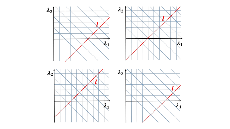
In our analysis of residues we will first state the complete results for the generic momenta, i.e. case E. For the three different families of poles, the residues are given by
| (5.4) | ||||
| (5.5) | ||||
| (5.6) | ||||
In the last family, the residue of the block at turns out to be proportional to the block with permuted and reflected momenta, i.e. with . For the first two families, however, the residues of blocks are not proportional to a block anymore, unless the spin becomes integer in which case
These relations for conformal blocks with integer mimic those of the Harish-Chandra functions, see table 2. Within our list of poles (cases A-D), there are two cases in which the residues of the first two families of poles are proportional to a single block. Actually, this happens in case D since the coefficient in front of the second Harish-Chandra function vanishes, see our discussion in the previous section, so that the block is actually given by a single Harish-Chandra function. In addition, it can also happen in case A for poles of the series and for those poles of series which do not collide to the ones from series. On the other hand, double poles arising from the colliding series of and singularities need a special treatment. Thus, once again, we are in agreement to the conformal group analysis of [32].
When double or triple pole collision appear in the cases A-C, the residues, of course, will look differently from the expressions we gave above for the generic case. In order to evaluate these such residues for an -th order pole at some point we use the standard prescription
in our explicit expansion (A) (or its -counterpart). Computing the corresponding residues for case A-C is in principle straightforward now, but we refrain from giving explicit expressions here. Our analysis provides a new view on the ’irregularities’ that were noticed in [32, 35], when poles of higher orders appear or residues are not proportional to blocks. From our ’analytically continued’ point of view, such problems are resolved into two separate issues. First, the blocks are linear combinations of twisted Harish-Chandra functions which for generic parameters leads to a linear combination of twisted Harish-Chandra functions rather than a simgle block. Furthermore, there is an issue of non-generic momenta for which care should be taken in defining Harish-Chandra functions as described in sections 3.2, 3.3 and appendix B.
Before we conclude this subsection, we want to discuss in a bit more detail in which respect our analysis advances the one in [32], where the authors analysed conformal blocks as sums over states in certain parabolic Verma modules of the conformal group. While Penedones et al. presented a nice general pattern of pole counting and calculating of residues of conformal blocks labeled by representations of the conformal group, we instead focused on the case of scalar blocks while applying the finer optics of Calogero-Sutherland scattering theory. Our analysis treats blocks as meromorphic functions in the labels of the intermediate field, i.e. the momenta for scalar blocks, so that we can really explore a full (complexified) parameter space in momenta .262626The restrictions we imposed, namely that the dimension is integer and that is positive, are both easy to lift. This also gives some new singularities, in particular the triple poles for odd dimension and half-integer . Blocks with non-integer spin have recently started to play an important role e.g. in the Froissart-Gribov type formula of [51], see also the next subsection. What we have seen here is just a first illustration of a recurrent theme in Calogero-Sutherland theory. In fact, the integrable DAHA [47] setting whose relation to conformal blocks we are developing is tailored to explorations of full complex parameter spaces. We will dwell on algebraic structures and their implications in a forthcoming paper [50]. At the same time, it seems to us that analytical continuation in dimension and representation labels would be difficult to achieve with the representation theoretic methods of [32], or at least requires to implement significant new technology such as the interpolating Karoubian categories for representation theories of conformal groups [79] to put it on a firm ground.
5.2 On the derivation of a Gribov-Froissart formula for CFT
In a recent paper [51], Caron-Huot derived a Lorentzian inversion formula that allows to obtain the operator product expansion coefficients from the discontinuity of the four-point correlation function , see also [52] for an alternative derivation. The formula actually extracts a function that is analytic in the spin . The mathematical counterpart/origin of formulas of Gribov-Froissart type goes under the name of Ramanujan’s master theorem, see [80] (p.297) and [81] for a more recent review. Related inversion formulas for Calogero-Sutherland Hamiltonians have been studied in the mathematical literature [82]. To explain the basic setup let us stress that the (twisted) Heckman-Opdam hypergeometric functions on the usual domain or the Lorentzian domain provide an orthonormal basis of wave functions that in many respects is similar to the basis of exponentials for functions on the real line. Just as the latter give rise to the usual Fourier transform, Heckman-Opdam functions define an interesting integral transform that has been investigated e.g. in [57, 65, 68, 83]. For the special case of , this transform, conventionally known as Jacobi (function) transform [61], has also been considered in the conformal bootstrap literature where it was dubbed “ space transform”, see [84, 85].
Questions that are natural to study for Fourier transforms are also natural to study for the integral transform that is obtained from (twisted) Heckman-Opdam functions. In particular, one may look at how the behaviour of a function is related to the asymptotic behavior of its transform in the parameters and for various choices of function spaces [86] on the Weyl chamber or the Lorentzian domain. A large body of such results in mathematics go under the name Tauberian theorems [87]. In the physics literature, similar issues were studied in [88, 89] by application of classical (Hardy-Littlewood and Wiener) Tauberian theorems for the Fourier transform, see also [90, 91, 92] for related physical arguments. In conformal field theory, these provide bounds on the asymptotic behaviour of the spectral density that arise from the short distance behaviour of the correlator. Wiener’s Tauberian theorem tailored272727A usual Wiener type Tauberian theorem states that the translations of an integrable function span a dense space iff its Fourier transform is everywhere non-zero. For Heckman-Opdam transforms the translation is replaced by a generalized translation that is determined by the positive convolution structure. to the case can be found in [93], while Tauberian theorems for special cases of Heckman-Opdam functions coming from representation theory appear in [94].282828In particular, for the case, it would be interesting to see whether the Jacobi transform Tauberian theorem of [93] can improve the conformal field theory analysis of [89] in order to constrain the subleading behaviour of spectral density and, perhaps, to show that the spectrum of the exchanged operators approaches the one of generalized free theory. It would also be nice to see if the case can provide a rigorous justification for results in [90, 91] on the lightcone limit, as approached in [89] through the usual Wiener Tauberian theorem.
A related line of research concerns Bochner-type positivity statements. In the case of ordinary Fourier(-Stiltjes) transform, the latter states that a function on a real line is a transform of a positive measure iff it is continuous and positive-definite. [95] Generalizations to the context of Heckman-Opdam theory are formulated in terms of positive convolution structures.[96] They were addressed in [97, 98] for , in [99] for and in [100] for , but with very specific choices of the multiplicities . This mathematical framework provides the natural context for Caron-Huot’s Froissart-Gribov formula. In fact, the Lorentzian inversion formula of [51] extracts positive operator product coefficients analytic in spin through an integral transform of the discontinuity of the correlation function . Instead of the usual Heckman-Opdam hypergeometric function , Caron-Huot obtains an integral transform defined by the block
| (5.7) |
i.e. is built as in eq. (4.3), but with replaced by . Similar integral transforms that are obtained from -hypergeometric functions in the terminology of section 3.4 have also been studied in the mathematical literature [101].
In order to derive the conformal Froissart-Gribov formula, Caron-Huot departs from the Euclidean inversion formula that goes back to the early harmonic analysis on the conformal group [7], see also [75], and performs an analytic continuation to Lorentzian signature. The Euclidean inversion formula involves a transform with the wave functions which we discussed at the end of section 3.4. Following [75], Caron-Huot denotes this function by the letter , a nice coincidence with our interpretation of it as a Euclidean hypergeometric function. In order to pass to Lorentzian signature, one needs a good understanding of the continuation of the functions . In in context of Heckman-Opdam theory this is provided my the monodromy matrices . Let us note that and coincide with the inverse of the monodromies which are encoded in eqs. (A.23) and (A.22) of [51]. From our discussion in section 3.4 we know that they provide an eight-dimensional representation of an affine braid group that satisfies Hecke relations (3.49). This insight provides significant algebraic control of the monodromy properties of Harish-Chandra (or pure, in the terminology of [51]) functions that can be exploited without ever using the explicit representation matrices. In order to demonstrate how constraining these algebraic properties are, we want to rephrase the main derivation of [51] (section 3.3) in our context.
Let us first review the general setup. It will be convenient to introduce the following functions
| (5.8) | |||||
| (5.9) |
that agree with the corresponding functions in [51] apart from the normalization. Caron-Huot studies the function in the complex -plane. In our space, the latter is given by an infinite strip that is perpendicular to the space in Figure 3 and intersects it along the line where , see the grey strip in Figure 6. We can parametrize this strip by a complex coordinate such that . The parameter is related to the variable used by Caron-Huot through the exponential map, i.e. . The region in which is mapped to while we can reach by sending to positive infinity.
The strip we have just described intersects the walls in six different places. In fact, as illustrated in Figure 6, thee are two intersections with the wall in . Intersections with the walls and , on the other hand, are located at and , respectively. After passing to the -plane, the intersections with the wall become the end-points of the t-channel cuts described by Caron-Huot. The intersections with map to the end-points of the u-channel cuts in the -plane.
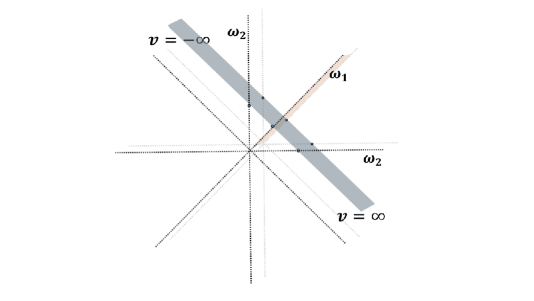
Caron-Huot now wants to continue the function to , i.e. . Along the way, one has to pass by the intersection with the walls and . While is regular at the wall , i.e. , it picks up some monodromy as it passes by . So, we can take the limit by looking at the function . According to our general characterization of , the function trivializes the monodromy , i.e.
| (5.10) |
Let us restrict our discussion to generic dimension , i.e. we assume that is not integer. As we explained at the end of the previous section, for such generic the function is a linear combination of two Harish-Chandra functions,
When we act with , two more Harish-Chandra functions appear, namely and . Because of the property (5.10) the corresponding functions combine into a single block . This new block that appeared while we continued through the wall to the region of small does not vanish in the limit and thereby it prevents further evaluation of the integral in [51].
The idea of Caron-Huot is to look for an appropriate combination of Harish-Chandra functions that vanish at and can cancel the unwanted divergent terms at . It is easy to see that there are two Harish-Chandra functions that vanish at , namely the functions and . From the corresponding functions and , see table 1, we can construct the block we introduced before in eq. (5.7). By construction, the function trivializes the monodromy , i.e.
In order to evaluate its behavior for small , one has to continue from large absolute values of to very small ones. Along the way, we pass the walls and again. Cancellation of the singular terms then means that there exist constants and such that
This is a precise formulation of Caron Huot’s condition (3.13) in [51] in the language we have set up. In order to illustrate how to derive such statements using algebra rather than the precise matrix elements the monodromy matrices, we want to prove, restricting to generic , a closely related statement, namely that there exist constants and such that, the following equation holds
| (5.11) |
In order to derive this claim we shall consider eq. (5.11) as a formula that allows us to construct the functions from as
| (5.12) |
Through a short computation using braid and Hecke relations of the monodromy matrices, see section 3.4, one may show that the function
which is proportional to the right hand side of the previous equation if , possesses the following properties
On the other hand it is easy to see that contains only six of the the eight Harish-Chandra functions since we apply at most two monodromy matrices to . Because is an eigenfunction of with unit eigenvalue we conclude that
In addition was shown to be an eigenfunction of with unit eigenvalue. This fact imposes strong constraints on the coefficients and . In fact, as in our discussion of at the end of section 3.4 we can conclude that is given by the expression after eq. (3.55) and . Hence, we have established our formula eq. (5.12) and thereby the equation (5.11) we set out to prove. In the argument we have only used braid and Hecke relations of the monodromy matrices along with the fact that the Harish-Chandra functions and are eigenfunctions of the monodromy with unit eigenvalue, a very particular feature of representations with integer spin and generic .
6 Conclusions
In this work we began to elaborate on the very fruitful relation between conformal blocks and wave functions of Calogero-Sutherland models that was uncovered in [49]. In our review of Heckman-Opdam theory we focused on features that may be understood from the quantum mechanical treatment of Calogero-Sutherland scattering states. More advanced properties of the Calogero-Sutherland model that relate to its (super-)integrability were not discussed. These will be briefly outlined below and then presented thoroughly in a forthcoming paper.[50]
Even without tools from integrability we were able to recover essentially all important results about scalar 4-point blocks. The basic objects in Heckman-Opdam theory are the Harish-Chandra functions. Special cases of these functions also appeared in the recent work [51] where they were called pure functions. Here we obtained a new series expansion for these functions that is valid for non-integer spin and we derived a number of important properties from it. In particular, we located all poles in -space, which is the space of conformal weights and spins, and we computed their residues. In addition, we reviewed the classical results of Heckman and Opdam on monodromy properties of Harish-Chandra functions. Some of the monodromy matrices were also computed independently for in [51]. Here, we learned in addition that they give rise to finite dimensional representation of an affine braid group of reflection type that factors through the corresponding Hecke algebra. This algebraic characterization of the monodromy properties of Harish-Chandra (or pure) functions led to a simple derivation of some central observations in [51]. Once we understood how conformal blocks are built out of Harish-Chandra functions, we were also able to rederive many important results on conformal blocks, see e.g. [25, 26, 32], from our new series expansion and the residue formulas for Harish-Chandra functions. In our discussion we focused on some of the most useful properties of blocks. There exist many other consequences of Heckman-Opdam theory that lead to additional insights, a few of which do not seem to be known in the conformal field theory literature.
We expect that the analytical toolkit we outlined in this paper will prove useful for various approaches to the analytical bootstrap, see in particular [102, 103, 104, 51, 85, 105, 106, 107] and references therein for some recent work. In particular, our explicit understanding of the properties of conformal blocks should provide better control over large spin expansions, sum rules for operator product coefficients and multi-twist operators.
What makes the connection with Calogero-Sutherland models even more useful is that the techniques we have described actually apply much beyond the theory of scalar 4-point blocks. The most immediate extension concerns the study of defect blocks. In fact, scalar 4-point blocks are a very special case of a larger set of conformal blocks that can be used to expand the correlation function of two conformal defects of dimension . Scalar 4-point blocks correspond to , i.e. a -dimensional defect should be considered as a pair of points. Correlations functions of two local fields in the presence of a -dimensional defect have received some attention for in [76] and more generally in [108]. These involve one and two cross ratios, respectively, and the corresponding blocks turn out to be identical to the ones we have studied here for and . More recently, Gadde also considered setups with which can involve a larger number of cross ratios [54]. As we will show in a forthcoming paper, the conformal blocks for such configurations of two defects can all be built from the Harish-Chandra functions of BCN Calogero-Sutherland models. Hence, many of the results and techniques we have described in section 3 and the appendices directly apply to such defect blocks.
Another direction concerns applications to spinning blocks. In [109] we have shown that the Casimir equations for spinning blocks in dimension also take the form of a Calogero-Sutherland eigenvalue problem, though with a matrix valued potential. This observation can be extended to arbitrary dimensions, see [110]. The theory of scattering states for such matrix valued potentials is not really developed, at least for the case of BCN root systems, but the general strategy we reviewed before should still apply. In the case of root system, a restricted set of matrix valued potentials is well understood [47] and some first steps were taken for the most generic ones in [111]. It would be very interesting to extend the results we have described above to matrix Calogero-Sutherland models for BC2 roots systems, i.e. to study their symmetries, the fundamental domain, monodromy representations, series expansions etc.
Further extensions to superblocks are also feasible. As long as sufficiently many of the external fields are in short (BPS) multiplets, the associated blocks are the same as for the bosonic conformal symmetry. In general, however, the theory of superblocks with external fields in long multiplets is much more involved. On the other hand, as was demonstrated in [112], crossing symmetry involving long multiplets is significantly more constraining when analysed in terms of superblocks rather than their bosonic decomposition. Hence, it seems worthwhile to develop a systematic theory of superblocks. We believe that the corresponding Casimir equations can still be rewritten as eigenvalue equations for a supersymmetric version of Calogero-Sutherland models so that much of the above could be extended to superblocks. This remains an interesting direction for future research.
Let us stress however, that even in the case of scalar 4-point functions we did not even come close to exploring all the existing features of the model. In fact, the most remarkable property of the Calogero-Sutherland model is its (super-)integrability. It furnishes a wealth of additional and very powerful algebraic structure. So far, the only algebra we have seen above was the Hecke algebra that appeared in the context of the monodromy representation. It acts in the -dimensional spaces of Harish-Chandra functions , i.e. in finite dimensional subspaces of functions which all possess the same eigenvalue of the Hamiltonian. This is just the tip of a true iceberg of algebraic structure.
In order to describe the contours of the remaining parts and thereby outline the content of our forthcoming paper [50], it is useful to consider the example of the very simplest quantum mechanical system, i.e. of a system of freely moving particles on the real line. The standard Hamiltonian of such a system is certainly integrable. Actually, can be built from a set of commuting first order operators as . Although Calogero-Sutherland particles are not free, they enjoy very similar properties. In fact, it is well known that the Calogero-Sutherland Hamiltonian for BCN roots systems can be constructed out of a set of commuting first order operators that are known as Dunkl operators. Of course, these Dunkl operators have to account for the non-trivial potentials in the Calogero-Sutherland model and hence possess a non-trivial dependence of the coordinates. Eigenfunctions of the Dunkl operators belong to a slighly larger class of non-symmetric Harish-Chandra functions. These are similar to the Harish-Chandra functions we discussed above except that they are no longer invariant under the action of the Weyl group on coordinates . Within the space of such non-symmetric Harish-Chandra functions, the Dunkl operators give rise to a systems of Knizhnik-Zamolodchikov-like first order differential equations.[113] Once these are solved, symmetric Harish-Chandra functions and in particular the conformal blocks can be obtained through an appropriate projection. The space of non-symmetric Harish-Chandra functions is acted upon by an infinite dimensional algebraic structure that is generated by elements of the Weyl group, Dunkl operators and multiplication with coordinates: The degenerate double affine Hecke algebra (DAHA) or trigonometric Cherednik algebra.[47] In addition to the monodromy algebra we have seen above, it contains generators that do not commute with the Hamiltonian and hence can relate eigenfunctions with different eigenvalues. In this sense, the degenerate DAHA is a spectrum generating symmetry.
This is not the end of the story. In order to prepare for its next chapter, we return to example of freely moving particles. The eigenfunctions in such a system possess a remarkable property: Namely, their dependence on the eigenvalues is the same as for the variables . This implies that are also eigenfunctions of a dual second order operator . We have put a superscript in this Hamiltonian since it controls dependence of the eigenfunctions on the eigenvalues of the first order operators . The dual Hamiltonian has precisely the same form as the original one. In this sense, the theory of a freely moving particles may be considered as self-dual. Some of these facts remain true for our Calogero-Sutherland model. As for free particles, the dependence of Calogero-Sutherland wave functions on the eigenvalued is controlled by a dual Hamiltonian . For the hyperbolic Calogero-Sutherland model, the latter is a second order difference operator that describes the so-called rational Ruijsenaars-Schneider model. [114, 115, 116] This dual Hamiltonian is also integrable, i.e. there is a set of first order difference equations that determines the dependence of eigenfunctions on the eigenvalues . In the case of the free particle we saw that the dual Hamiltonian had the same form as . This is is sharp contrast to the case of the hyperbolic Calogero-Sutherland system where the dual theory is controlled by difference rather than differential equations. It turns out, however, that the setup can be -deformed such that the self-duality is restored. In order to so so, the rational Ruijsenaars-Schneider model is deformed into the trigonometric one. After this deformation, the dependence of eigenfunctions on both sets of variables is controlled by the same type of difference equations. Upon deformation the degenerate DAHA we briefly mentioned at the end of the previous paragraph becomes a full fledged DAHA. All this will be explained in detail in our forthcoming paper [50] along with a number of applications.
7 Acknowledgements
We wish to thank T. Bargheer, S. Caron-Huot, A. Gadde, M. Hogervorst, M. Honda, Z. Komargodski, S. Komatsu, P. Kravchuk, M. Lemos, P. Liendo, G. Mack, D. Mazac, C. Meneghelli, V. Narovlansky, D. Poland, L. Rastelli, B. van Rees, N. Reshetikhin, S. Shatashvili, D. Simmons-Duffin, W. Skiba, Zh. Sobko, G. Torrents and R. Yacoby for useful conversations and/or remarks and especially Ivan Cherednik for illuminating discussions. We are also grateful to the the participants and organizers of the ’Back to bootstrap 2016’, ’Bootstrap 2017’ and ’Strings 2017’ conferences, of the 2016 Les Houches Summer School on Integrability and of the 2017 Cargese Summer School for the occasion to discuss our work. MI thanks the DESY Theory Group, the Simons Center for Geometry and Physics, Yale University, the Institute for Advanced Study, Duke University and the Math Department of Chapel Hill University, North Carolina, for a stimulating environment and hospitality during various stages of this work. MI is supported in part by Israel Science Foundation (grant number 1989/14), by the ERC STG grant 335182 and by a Koshland Postdoctoral fellowship, partially financed by the Koshland Foundation.
Appendix A - and -expansions for Harish-Chandra function
As far as we know, the formulas for Harish-Chandra functions in this section are new. Let us recall here that conformal blocks are obtained via formulas (4.3) from twisted Harish-Chandra functions, which are related to the Harish-Chandra function by a simple phase shift as given in our eq. (3.52). According to [67], the resulting expansion is convergent for generic on the entire shifted fundamental domain.
We start from the formula (3.2) in the main text. For the twisted Harish-Chandra function it takes the form
| (A.1) | ||||
Here an in the following we use the shorthand and . Before we plunge into details, let us first outline its derivation.
The key is an observation from [49] where we directly related scalar conformal blocks to degeneration of virtual Koornwinder polynomials [117]. Due to the fast (and still on-going) progress in the end of 1990’s, combinatorial aspects of Koornwinder polynomials are quite well-studied, in particular the so-called binomial expansion of Koornwinder polynomials that were obtained in [118]. Now we will factor this connection through the connection to Harish-Chandra functions of specialized parameters (for , it means looking at Harish-Chandra functions with integer) and then will analytically continue in these parameters. To start with, the (non-symmetric ) Harish-Chandra functions are related to Macdonald-Koornwinder polynomials in [119]. One may write down a binomial formula for virtual Koornwinder polynomials [117] and then use combinatorial expansions for the interpolating polynomials it contains (combinatorial expansions of interpolation Macdonald polynomials can be found in [118] and the degeneration to interpolation Jack polynomials in [120]), see [121] for a nice review. Next one has to perform an analytical continuation of the resulting formula to non-integer differences between the row lengths of Young diagrams. By analysing the asymptotics, one may note that the resulting series expansion is a linear combination of asymptotically free solutions (-Harish-Chandra functions), corresponding to a subgroup of the Weyl group. It is then possible to single out a solution with the correct asymptotics.
This way of obtaining explicit series expansions in , which solves a rather complicated recurrence relation (3.18) for expansion coefficients (after one passes to -variable), seems to work, provided one has sufficient control of the analytical continuation of the constituents of the binomial expansion, for any Harish-Chandra function. A degeneration is possible at any step, depending rather on convenience (purely formally, one can take the limit at any point of the derivation, but sometimes this should be justified with more care). Regardless of that, the complexity of explicit computation increases very fast with , and we are not aware of any closed form expansion of a generic Harish-Chandra function valid for any .
Let us look at case in more detail. The summand of a generalized binomial formula for virtual Koornwinder polynomials (see [117], formula (7.32)) contains a generalized binomial coefficient (which is proportional to a interpolation Macdonald polynomial), a (virtual) -interpolation Macdonald polynomial and some remaining ratios of -Pochhammer symbols. To avoid heavy expressions, we will send now. This degeneration has different consequences for the two interpolation polynomials: the one entering the generalized binomial coefficient will go to a interpolation Jack polynomial, whereas the virtual -interpolation polynomial will go to a virtual Jack polynomial (’virtual’ – here just means having a monomial of non-integer powers in front of Gegenbauer polynomial) [120].
Using explicit expressions from [117] and a combinatorial expansion for the -interpolation Jack polynomial from [118] combined with [120], one can see that the generalized binomial coefficient (undeformed) is proportional to
which we just related to a balanced appearing in eq. (3.2) via a Whipple transformation [60], combined with inverting of summation index. Clearly, the analytical continuation in of the function on the right-hand side will not change anything (the series will stay terminating), unlike the continuation of the one on the left (there the series is terminating for integer and becomes non-terminating for non-integer, so another term should appear, see [63] for a full account on the symmetries of hypergeometric function).
The ’virtual’ Jack polynomial, which as we said for , is just a product of a monomial and a Gegenbauer polynomial, upon analytical continuation in also becomes a non-terminating series
| (A.2) | ||||
By using a particular quadratic transformation [60] (chapter 3.1) for , this can also be written as
| (A.3) | ||||
Let us dress this back with the above binomial coefficient (and other Pochhammers from the generalized binomial formula that we didn’t display), take the first summand and strip off the prefactor. This then gives us the (twisted)292929As the domain we work on is . Harish-Chandra series decomposition as
Notice that, in accord with the general definition of Harish-Chandra functions, this series development is explicitly -invariant, the non-trivial symmetry here being exactly since the symmetry with respect to the subgroup was already taken into account by our definition of -variables in eq. (2.28). Of course, taking asymptotics at infinity breaks this symmetry explicitly.
To bring the last expansion to the form in eq. (A), one should apply another quadratic transformation of the form
| (A.4) |
Here we run into a subtlety (first noticed by Gauss himself) which is sometimes encountered in working with quadratic transformations: The absolute value of in the above formula should be less than one for it to be valid. Although one might imagine a wider applicability range by analytical continuation, in fact it does not happen. Actually, a second term should appear in the quadratic transformation to correct it in the latter case: Compare formula (3.1.3) in [60] and ex. 6 for chapter 3 ibid.303030When substituted into the Harish-Chandra expansion, the emergence of a second term can be seen as appropriate to give a continuation of the Harish-Chandra function past the wall . In other words, it gives the action of monodromy matrix , see subsection 3.4. So, we are forced to explicitly choose between two expansion domains related via and to break the symmetry by setting ( for ) along with , finally arriving at eq. (A).
The expansion (A) is absolutely convergent when
| (A.5) |
as can be checked by using classical Horn’s theorem [122]. For the convergence analysis, it is actually more convenient to pass to a different, resummed form
| (A.6) |
To obtain this formula from eq. (A), one can use an identity
| (A.7) |
which follows from Bailey lemma [60]. It is also instrumental to keep in mind another particular presentation of the -expansion which can be obtained by combining Whipple’s identity and symmetry of a terminating well-poised function [63]
| (A.8) | |||
To complete our discussion of the -expansions, let us finally spell out the one summing over the cone of positive roots, which makes the partial ordering of terms in the series manifest. To achieve this goal, we again use eq. (A.7) and obtain
| (A.9) | ||||
Notice that the Pochhammers of index in the first two lines of the inner double sum are "almost well-poised", i.e. the upper and the lower parameters are related by with . This implies that such a double sum should be a close two-variable analogue of a well-poised function. To see this somewhat more clearly, the last line can be additionally rewritten through Whipple identity as
In order to obtain expansions in the ’radial’ coordinates ( or ), we again start with eq. (A). For generic values of parameters, the -expansion then can be derived in the same way as in the example from the main text, i.e. through the use of a binomial theorem folowed by a change of summation indices
| (A.10) | |||
This form seems to be most useful for getting an expansion of the blocks in Jack (Gegenbauer) polynomials of radial variables, which explicitly solves the recursion relations given in [62]. We will not present the result here, as we do not use it. Instead, by changing summation indices and employing again the resummation identity (A.7), we obtain an explicit, manifestly partially ordered (i.e., over the -cone of positive roots) expansion of Harish-Chandra functions in the coordinates as313131The coefficient of the powers in this expansion, i.e. the inner triple sum of Pochhammer symbols times the balanced function, is, of course, a finite sum. It can be easily written as a product of Pochhammer quotients and a quadruple hypergeometric polynomial.
| (A.11) | ||||
This is the main result of this section. As the coefficient of the expansion term solves the recursion relation (3.18), according to general theorems of Heckman and Opdam [57] for generic values of the expansion is convergent on the whole domain and can be analytically continued to the entire (complex) fundamental domain. The expansion (A) combined with Heckman-Opdam results gives a full control over the analytical properties of the Harish-Chandra functions.
The two expansions in coordinates above can be recast in many equivalent forms. All of them can in principle be regarded as instances of sextuple Srivastava-Daoust hypergeometric functions [123], a rather general class of analogues of hypergeometric functions. Since information on the analytical behaviour of a generic member of this family seems to be quite scarce, it is fortunate that we have the well-developed Heckman-Opdam theory at our disposal (and a root symmetry at the root of it). We are not aware of any significant simplification of the above formula for generic values of the parameters, it would be interesting to prove this rigorously.
To conclude this appendix, let us comment on the case of general . We claim that in fact all the building blocks required for writing down the expansions are already present here, although writing up a general formula requires extra work along the lines described in the beginning of the appendix. It appears that such general expansions of Harish-Chandra functions will involve and summations, which are numbers of roots of the root system and of its corresponding reduced root subsystem ( or ), especially when looking at such beautifully symmetric expansions as eq. (A). Clearly, for we get back -summations and -summations of the above.
We conjecture that these numbers of summations are minimal possible for the generic values of parameters and, moreover, that the same is true also for Harish-Chandra functions of other root systems, of which the ones associated to exceptional root systems are probably mathematically most interesting, since they cannot be obtained as special cases or limits of the BC case. E.g. for Harish-Chandra function this would imply a minimum of / summations. As such explicit general expansions are not yet available, it is an interesting mathematical problem to solve. As explained in [53], the Harish-Chandra functions describe conformal blocks of parallel defects of codimension (in ambient space of a sufficiently high dimensionality). So, such expansions are of potential interest for the conformal bootstrap programme, provided there is a corresponding analogue of crossing symmetry for such defects.
Appendix B Alternative expansions for integer spin
The aim of this appendix is to specialize our general expansion (A) to integer spin and to rewrite it as an expansion in the usual cross ratios and , or rather variables and . The latter can then be compared with existing expressions from other approaches, such as the shadow or the embedding formalism.
Before we study Harish-Chandra series for such special values of the parameters, we want to make some general comments. Actually, one has to be a bit careful when evaluating formulas that are valid for generic values of the parameters, like the ones for Harish-Chandra functions in the previous appendix, at special values of the parameters such as the momenta . In order to do so, one should first take a limit for the multiplicities, and only then for the momenta (i.e. the continued spin or conformal dimension). In other words, if we want to study blocks/Harish-Chandra functions for particular spins (or twists) through the general series expansions, our prescription is to fix the dimension and conformal weights of external fields first and only then, after carefully taking into account all implications on the summation range, to send the spin (or twist) to some particular value. This recipe is directly related to the fact that an (appropriately normalized) Harish-Chandra function is an entire function of its multiplicities, but can have simple poles in (and further subtleties related to its series expansion for along specific affine hyperplanes, see subsections 3.2, 3.3, 5.1). The opposite order of limits, provided it exists at all, also gives some solution of the Calogero-Sutherland problem, but one that may be a non-trivial linear combination of all the Harish-Chandra functions. The prescription we propose here is the same as usually used when taking limits in formulas for the hypergeometric function (i.e. for ) to special values of its parameters [124]: when e.g. one upper and one lower parameter are negative integers, one takes
rather than
where are positive integers and is generic. One can show that the second function is a linear combination of the first and its shadow.
After these introductory remarks we now want to start with our general formula (A) and set , i.e. . For the moment we shall assume that the dimension is not even so that upon specializing , the twisted Harish-Chandra function is actually just equal to a block, up to a normalizing prefactor . By applying a Whipple transformation [60] to the inner function in eq. (A), we can perform a sum via Saalschütz formula, yielding323232The analysis by Horn’s theorem [122] shows that the absolute convergence for this series representation of the twisted Harish-Chandra function in fact takes place on a the extended domain and . This is, of course, consistent with the fact that the single twisted Harish-Chandra function for generic dimension, being proportional to a block, is bound to be regular at the wall according to our discussion in subsection 5.1.
| (B.1) |
By changing the order of summation, we can rewrite this expression as
The inner well-poised is now to be transformed to another one using the symmetry of this function. Namely, we can apply a particular identity labeled by Bailey [63], employ the series representation for the resulting inner function and shift the summation indices. This leads to
| (B.2) | |||
where and summations were absorbed into the two hypergeometric functions. Using Chu-Vandermonde identity [60] in the form
and shifting summation indices, we can rewrite our expression further as
| (B.3) | |||
so that for the inner () sum we can now use a beautiful identity of Burchnall-Chaundy ([125], formula (50))
| (B.4) | ||||
(provided both sides converge or assuming analytical continuation), and finally arrive at333333Note that, while previous manipulations just reshuffled summation order in an absolutely convergent series, the application of Burchnall-Chaundy formula changes the domain of (absolute) convergence which now becomes .
| (B.5) |
where are the usual cross ratios defined in eq. (4.2). As in section 4, we identify , . Once we pass to conformal blocks using our relation (4.3), we recognize formula (3.32) in [26] (see also [24]). Dolan and Osborn obtained this formula from the shadow formalism by calculating the corresponding integrals via Mellin transform, ignoring all pole terms form the shadow contributions. As noticed e.g. in [126, 24], this double hypergeometric expression (B.5) can be rewritten as a linear combination of two Appell functions.343434Notice that the convergence region after using this connection formula changes to , so a diagonal wall is in fact re-introduced. It is clear that we can lift our restriction on and admit even values, literally repeating the above calculation for the scalar exchange block which for even is composed from two twisted Harish-Chandra functions.
The type of analysis we have presented here and in particular the use of Burchnall-Chaundy type formulas, generalizes much beyond the specific case analysed here and allows to relate expressions from our approach to those obtained through the shadow formalism [26] or results from the embedding formalism [29, 127, 128]. In particular, we can go through the same steps for any spin (and ’push out’ the finite summations associated to the spin being integer) to obtain finite sums of double hypergeometric functions of Srivastava-Daoust (i.e. generalized Kampé de Fériet) type [123]. While the resulting expressions can be used to compare with results from other approaches, we want to stress that the expansion formulas we have derived in appendix A and their direct specializations are typically simpler than those that are obtained by other techniques.
References
- [1] G. Mack and A. Salam, Finite component field representations of the conformal group, Annals Phys. 53 (1969) 174–202.
- [2] A. M. Polyakov, Conformal symmetry of critical fluctuations, JETP Lett. 12 (1970) 381–383.
- [3] S. Ferrara, A. F. Grillo, G. Parisi and R. Gatto, Covariant expansion of the conformal four-point function, Nucl. Phys. B49 (1972) 77–98.
- [4] S. Ferrara, A. F. Grillo and R. Gatto, Tensor representations of conformal algebra and conformally covariant operator product expansion, Annals Phys. 76 (1973) 161–188.
- [5] A. M. Polyakov, Nonhamiltonian approach to conformal quantum field theory, Zh. Eksp. Teor. Fiz. 66 (1974) 23–42.
- [6] G. Mack, Duality in quantum field theory, Nucl. Phys. B118 (1977) 445–457.
- [7] V. K. Dobrev, G. Mack, V. B. Petkova, S. G. Petrova and I. T. Todorov, Harmonic Analysis on the n-Dimensional Lorentz Group and Its Application to Conformal Quantum Field Theory, Lect. Notes Phys. 63 (1977) 1–280.
- [8] A. A. Belavin, A. M. Polyakov and A. B. Zamolodchikov, Infinite Conformal Symmetry in Two-Dimensional Quantum Field Theory, Nucl. Phys. B241 (1984) 333–380.
- [9] R. Rattazzi, V. S. Rychkov, E. Tonni and A. Vichi, Bounding scalar operator dimensions in 4D CFT, JHEP 12 (2008) 031, [0807.0004].
- [10] S. El-Showk, M. F. Paulos, D. Poland, S. Rychkov, D. Simmons-Duffin and A. Vichi, Solving the 3D Ising Model with the Conformal Bootstrap, Phys. Rev. D86 (2012) 025022, [1203.6064].
- [11] S. El-Showk, M. F. Paulos, D. Poland, S. Rychkov, D. Simmons-Duffin and A. Vichi, Solving the 3d Ising Model with the Conformal Bootstrap II. c-Minimization and Precise Critical Exponents, J. Stat. Phys. 157 (2014) 869, [1403.4545].
- [12] F. Kos, D. Poland and D. Simmons-Duffin, Bootstrapping Mixed Correlators in the 3D Ising Model, JHEP 11 (2014) 109, [1406.4858].
- [13] D. Simmons-Duffin, A Semidefinite Program Solver for the Conformal Bootstrap, JHEP 06 (2015) 174, [1502.02033].
- [14] F. Kos, D. Poland, D. Simmons-Duffin and A. Vichi, Precision Islands in the Ising and Models, JHEP 08 (2016) 036, [1603.04436].
- [15] A. Dymarsky, F. Kos, P. Kravchuk, D. Poland and D. Simmons-Duffin, The 3d Stress-Tensor Bootstrap, 1708.05718.
- [16] F. Kos, D. Poland and D. Simmons-Duffin, Bootstrapping the vector models, JHEP 06 (2014) 091, [1307.6856].
- [17] F. Kos, D. Poland, D. Simmons-Duffin and A. Vichi, Bootstrapping the O(N) Archipelago, JHEP 11 (2015) 106, [1504.07997].
- [18] L. Iliesiu, F. Kos, D. Poland, S. S. Pufu, D. Simmons-Duffin and R. Yacoby, Bootstrapping 3D Fermions, JHEP 03 (2016) 120, [1508.00012].
- [19] L. Iliesiu, F. Kos, D. Poland, S. S. Pufu and D. Simmons-Duffin, Bootstrapping 3D Fermions with Global Symmetries, 1705.03484.
- [20] R. Rattazzi, S. Rychkov and A. Vichi, Bounds in 4D Conformal Field Theories with Global Symmetry, J. Phys. A44 (2011) 035402, [1009.5985].
- [21] D. Poland, D. Simmons-Duffin and A. Vichi, Carving Out the Space of 4D CFTs, JHEP 05 (2012) 110, [1109.5176].
- [22] S. M. Chester and S. S. Pufu, Towards bootstrapping QED3, JHEP 08 (2016) 019, [1601.03476].
- [23] S. M. Chester and S. S. Pufu, Anomalous dimensions of scalar operators in QED3, JHEP 08 (2016) 069, [1603.05582].
- [24] F. A. Dolan and H. Osborn, Conformal four point functions and the operator product expansion, Nucl. Phys. B599 (2001) 459–496, [hep-th/0011040].
- [25] F. A. Dolan and H. Osborn, Conformal partial waves and the operator product expansion, Nucl. Phys. B678 (2004) 491–507, [hep-th/0309180].
- [26] F. A. Dolan and H. Osborn, Conformal Partial Waves: Further Mathematical Results, 1108.6194.
- [27] M. S. Costa, J. Penedones, D. Poland and S. Rychkov, Spinning Conformal Correlators, JHEP 11 (2011) 071, [1107.3554].
- [28] M. S. Costa, J. Penedones, D. Poland and S. Rychkov, Spinning Conformal Blocks, JHEP 11 (2011) 154, [1109.6321].
- [29] D. Simmons-Duffin, Projectors, Shadows, and Conformal Blocks, JHEP 04 (2014) 146, [1204.3894].
- [30] F. Rejon-Barrera and D. Robbins, Scalar-Vector Bootstrap, JHEP 01 (2016) 139, [1508.02676].
- [31] M. S. Costa and T. Hansen, Conformal correlators of mixed-symmetry tensors, JHEP 02 (2015) 151, [1411.7351].
- [32] J. Penedones, E. Trevisani and M. Yamazaki, Recursion Relations for Conformal Blocks, JHEP 09 (2016) 070, [1509.00428].
- [33] A. Castedo Echeverri, E. Elkhidir, D. Karateev and M. Serone, Deconstructing Conformal Blocks in 4D CFT, JHEP 08 (2015) 101, [1505.03750].
- [34] L. Iliesiu, F. Kos, D. Poland, S. S. Pufu, D. Simmons-Duffin and R. Yacoby, Fermion-Scalar Conformal Blocks, JHEP 04 (2016) 074, [1511.01497].
- [35] M. S. Costa, T. Hansen, J. Penedones and E. Trevisani, Radial expansion for spinning conformal blocks, JHEP 07 (2016) 057, [1603.05552].
- [36] M. S. Costa, T. Hansen, J. Penedones and E. Trevisani, Projectors and seed conformal blocks for traceless mixed-symmetry tensors, JHEP 07 (2016) 018, [1603.05551].
- [37] A. Castedo Echeverri, E. Elkhidir, D. Karateev and M. Serone, Seed Conformal Blocks in 4D CFT, JHEP 02 (2016) 183, [1601.05325].
- [38] D. Karateev, P. Kravchuk and D. Simmons-Duffin, Weight Shifting Operators and Conformal Blocks, 1706.07813.
- [39] P. Kravchuk and D. Simmons-Duffin, Counting Conformal Correlators, 1612.08987.
- [40] P. Kravchuk, Casimir recursion relations for general conformal blocks, 1709.05347.
- [41] F. Calogero, Solution of the one-dimensional N body problems with quadratic and/or inversely quadratic pair potentials, J. Math. Phys. 12 (1971) 419–436.
- [42] B. Sutherland, Exact results for a quantum many body problem in one dimension. 2., Phys. Rev. A5 (1972) 1372–1376.
- [43] J. Moser, Three integrable Hamiltonian systems connected with isospectral deformations, Adv. Math. 16 (1975) 197– 220.
- [44] G. J. Heckman, Root systems and hypergeometric functions. I-II, Compositio Mathematica 64 (1987) 329–373 and 353–373.
- [45] E. M. Opdam, Root systems and hypergeometric functions III-IV, Compositio Mathematica 67 (1988) 21–49 and 191–209.
- [46] T. Koornwinder, Orthogonal polynomials in two variables which are eigenfunctions of two algebraically independent partial differential operators, I-IV, Indag. Math. 36 (1974) 48–66 and 358–381.
- [47] I. Cherednik, Double Affine Hecke Algebras. Cambridge University Press, 2005.
- [48] I. Macdonald, Affine Hecke Algebras and Orthogonal Polynomials. Cambridge tracts in mathematics. Cambridge University Press, 2003.
- [49] M. Isachenkov and V. Schomerus, Superintegrability of -dimensional Conformal Blocks, Phys. Rev. Lett. 117 (2016) 071602, [1602.01858].
- [50] M. Isachenkov and V. Schomerus, Integrability of Conformal Blocks II: Algebraic Structures, in preparation, .
- [51] S. Caron-Huot, Analyticity in Spin in Conformal Theories, JHEP 09 (2017) 078, [1703.00278].
- [52] D. Simmons-Duffin, D. Stanford and E. Witten, A spacetime derivation of the Lorentzian OPE inversion formula, 1711.03816.
- [53] V. Schomerus, Harmony of defect blocks, talk given at the workshop ’Boundary and Defect Conformal Field Theory: Open Problems and Applications’, Chicheley Hall, Sep 2017.
- [54] A. Gadde, Conformal constraints on defects, 1602.06354.
- [55] M. Fukuda, N. Kobayashi and T. Nishioka, Operator product expansion for conformal defects, 1710.11165.
- [56] G. Pöschl and E. Teller, Bemerkungen zur Quantenmechanik des anharmonischen Oszillators, Z. Phys. 83 (1933) 143–151.
- [57] G. Heckman and H. Schlichtkrull, Harmonic Analysis and Special Functions on Symmetric Spaces. Academic Press, 1994.
- [58] V. I. Danilov, The geometry of toric varieties, Uspekhi Mat. Nauk 33 (1978) 85–134, 247.
- [59] T. Oda, Convex Bodies and Algebraic Geometry. Springer-Verlag, 1988.
- [60] G.E. Andrews, R. Askey and R. Roy, Special Functions. Cambridge University Press, 1999.
- [61] T. Koornwinder, Jacobi Functions and Analysis on Noncompact Semisimple Lie Groups, Special Functions: Group Theoretical Aspects and Applications (1984) 1–85.
- [62] M. Hogervorst and S. Rychkov, Radial Coordinates for Conformal Blocks, Phys. Rev. D87 (2013) 106004, [1303.1111].
- [63] W. Bailey, Generalized hypergeometric series. Cambridge tracts in mathematics and mathematical physics. The University Press, 1935.
- [64] N. Shimeno, Formula for the hypergeometric functions of type , Pacific J. of Math. 236 .
- [65] E. M. Opdam, Part I: Lectures on Dunkl Operators, vol. Volume 8 of MSJ Memoirs, pp. 2–62. The Mathematical Society of Japan, Tokyo, Japan, 2000. 10.2969/msjmemoirs/008010C010.
- [66] S. G. Gindikin and F. I. Karpelevich, Plancherel measure for symmetric Riemannian spaces of non-positive curvature, Soviet Math. Dokl. 3 (1962) 962–965.
- [67] A. Pasquale, Asymptotic analysis of -hypergeometric functions, Inventiones mathematicae 157 (2004) 71–122.
- [68] E. M. Opdam, Harmonic analysis for certain representations of graded Hecke algebras, Acta Math. 175 (1995) 75–121.
- [69] N. V. Dũng, The fundamental groups of the spaces of regular orbits of the affine Weyl groups, Topology 22 (1983) 425 – 435.
- [70] E. Brieskorn, Die Fundamentalgruppe des Raumes der regulären Orbits einer endlichen komplexen Spiegelungsgruppe, Inventiones mathematicae 12 (1971) 57–61.
- [71] H. van der Lek, The homotopy type of complex hyperplane complements. Ph.D. Thesis, Nijmegen, 1983.
- [72] H. van der Lek, Extended Artin groups, Proc. Symp. Pure Math. 40.2 (1981) 117–122.
- [73] P. Deligne, Les immeubles des groupes de tresses généralisés, Inventiones mathematicae 17 (1972) 273–302.
- [74] E. M. Opdam, An analogue of the Gauss summation formula for hypergeometric functions related to root systems, Math. Z. 212 (1993) 313–336.
- [75] M. S. Costa, V. Gonçalves and J. Penedones, Conformal Regge theory, JHEP 12 (2012) 091, [1209.4355].
- [76] P. Liendo, L. Rastelli and B. C. van Rees, The Bootstrap Program for Boundary , JHEP 07 (2013) 113, [1210.4258].
- [77] F. Hartogs, Einige Folgerungen aus der Cauchyschen Integralformel bei Funktionen mehrerer Veränderlichen, Sitzungsberichte der Königlich Bayerischen Akademie der Wissenschaften zu München 36 (1906) 223–242.
- [78] W. Osgood, Topics in the theory of functions of several complex variables. New York: Dover Publications, 1966.
- [79] P. Deligne, ‘Catégories tannakiennes’ in the Grothendieck Festschrift: a collection of articles written in honor of the 60th birthday of A. Grothendieck, pp. 111–195. Birkhäuser Boston, 1990.
- [80] B. Berndt, Ramanujan’s Notebooks, Part I. Springer-Verlag New York, 1985.
- [81] T. Amdeberhan, O. Espinosa, I. Gonzalez, M. Harrison, V.H. Moll and A. Straub, Ramanujan’s Master Theorem, The Ramanujan Journal 29 (Dec, 2012) 103–120.
- [82] G. Olafsson and A. Pasquale, Ramanujan’s Master Theorem for the Hypergeometric Fourier Transform Associated with Root Systems, J. Fourier Analysis and Applications 19 (6) (2013) 1150–1183, [1211.0024].
- [83] I. Cherednik, Inverse Harish-Chandra transform and difference operators, International Mathematics Research Notices 1997 (1997) 733–750.
- [84] M. Hogervorst, Crossing Kernels for Boundary and Crosscap CFTs, 1703.08159.
- [85] M. Hogervorst and B. C. van Rees, Crossing Symmetry in Alpha Space, 1702.08471.
- [86] B. Schapira, Contributions to the hypergeometric function theory of Heckman and Opdam: sharp estimates, Schwartz space, heat kernel, Geom. and Func. Analysis 18 (2008) 222–250.
- [87] J. Korevaar, Tauberian Theorems. Springer-Verlag Berlin Heidelberg, 2004.
- [88] D. Pappadopulo, S. Rychkov, J. Espin and R. Rattazzi, OPE Convergence in Conformal Field Theory, Phys. Rev. D86 (2012) 105043, [1208.6449].
- [89] J. Qiao and S. Rychkov, A tauberian theorem for the conformal bootstrap, 1709.00008.
- [90] A. L. Fitzpatrick, J. Kaplan, D. Poland and D. Simmons-Duffin, The Analytic Bootstrap and AdS Superhorizon Locality, JHEP 12 (2013) 004, [1212.3616].
- [91] Z. Komargodski and A. Zhiboedov, Convexity and Liberation at Large Spin, JHEP 11 (2013) 140, [1212.4103].
- [92] A. L. Fitzpatrick, J. Kaplan and M. T. Walters, Universality of Long-Distance AdS Physics from the CFT Bootstrap, JHEP 08 (2014) 145, [1403.6829].
- [93] L. Jianming and Z. Weixing, A Wiener-Tauberian theorem for Fourier-Jacobi transform, Approximation Theory and its Applications 13 (Jun, 1997) 97–104.
- [94] E. K. Narayanan and A. Sitaram, Analogues of the Wiener-Tauberian and Schwartz theorems for radial functions on symmetric spaces, ArXiv e-prints (2009) , [0905.3018].
- [95] S. Bochner, Vorlesungen über Fouriersche Integrale. Leipzig: Akademische Verlagsgesellschaft, 1932.
- [96] C. Berg, J.P.R. Christensen, P. Ressel, Harmonic Analysis on Semigroups. Springer-Verlag, NY, 1984.
- [97] M. Flensted-Jensen and T. Koornwinder, The convolution structure for Jacobi function expansions, Arkiv för Matematik 11 (Dec, 1973) 245–262.
- [98] M. Flensted-Jensen and T. H. Koornwinder, Jacobi functions: The addition formula and the positivity of the dual convolution structure, Arkiv för Matematik 17 (Dec, 1979) 139.
- [99] K. Trimeche, The positivity of the transmutation operators associated to the Cherednik operators for the root system , Math. J. of Okuyama University 58 (2016) 183–198.
- [100] Margit Rösler, Positive convolution structure for a class of Heckman-Opdam hypergeometric functions of type BC, Journal of Functional Analysis 258 (2010) 2779 – 2800.
- [101] G. Ólafsson and A. Pasquale, Paley–Wiener Theorems for the -Spherical Transform: An Overview, Acta Applicandae Mathematica 81 (2004) 275–309.
- [102] L. F. Alday, Solving CFTs with Weakly Broken Higher Spin Symmetry, JHEP 10 (2017) 161, [1612.00696].
- [103] D. Mazac, Analytic bounds and emergence of AdS2 physics from the conformal bootstrap, JHEP 04 (2017) 146, [1611.10060].
- [104] D. Simmons-Duffin, The Lightcone Bootstrap and the Spectrum of the 3d Ising CFT, JHEP 03 (2017) 086, [1612.08471].
- [105] D. Li, D. Meltzer and D. Poland, Conformal Bootstrap in the Regge Limit, 1705.03453.
- [106] M. S. Costa, T. Hansen and J. Penedones, Bounds for OPE coefficients on the Regge trajectory, 1707.07689.
- [107] D. Jafferis, B. Mukhametzhanov and A. Zhiboedov, Conformal Bootstrap At Large Charge, 1710.11161.
- [108] M. Billò, V. Gonçalves, E. Lauria and M. Meineri, Defects in conformal field theory, JHEP 04 (2016) 091, [1601.02883].
- [109] V. Schomerus, E. Sobko and M. Isachenkov, Harmony of Spinning Conformal Blocks, JHEP 03 (2017) 085, [1612.02479].
- [110] V. Schomerus and E. Sobko, From Spinning Conformal Blocks to Matrix Calogero-Sutherland Models, 1711.02022.
- [111] N. Reshetikhin, Degenerate integrability of quantum spin Calogero-Moser systems, Lett. Math. Phys. 107 (2017) 187–200, [1510.00492].
- [112] M. Cornagliotto, M. Lemos and V. Schomerus, Long Multiplet Bootstrap, JHEP 10 (2017) 119, [1702.05101].
- [113] I. Cherednik, Quantum knizhnik-zamolodchikov equations and affine root systems, Comm. Math. Phys. 150 (1992) 109–136.
- [114] S. N. M. Ruijsenaars and H. Schneider, A New Class of Integrable Systems and Its Relation to Solitons, Annals Phys. 170 (1986) 370–405.
- [115] J. F. van Diejen, Integrability of difference Calogero-Moser systems, Journal of Mathematical Physics 35 (1994) 2983–3004.
- [116] J. F. van Diejen, Deformations of Calogero-Moser systems and finite Toda chains, Theoretical and Mathematical Physics 99 (May, 1994) 549–554.
- [117] E. Rains, -symmetric polynomials, Transformation Groups 10 (2005) 63–132.
- [118] A. Okounkov, BC-type interpolation Macdonald polynomials and binomial formula for Koornwinder polynomials, Transformation Groups 3 (1998) 181–207.
- [119] M. van Meer and J. Stokman, Double Affine Hecke Algebras and Bispectral Quantum Knizhnik-Zamolodchikov Equations, International Mathematics Research Notices 2010 (2010) 969–1040.
- [120] J. V. Stokman and T. H. Koornwinder, Limit Transitions for BC Type Multivariable Orthogonal Polynomials, 2005.
- [121] T. H. Koornwinder, Okounkov’s BC-type interpolation Macdonald polynomials and their q=1 limit, ArXiv e-prints (Aug., 2014) , [1408.5993].
- [122] J. Horn, Über die Convergenz der hypergeometrischen Reihen zweier und dreier Veränderlichen, Math. Ann. 34 (1889) 544–600.
- [123] H. Srivastava and M. Daoust, Certain generalized Neumann expansions associated with the Kampé de Fériet function, Indag. Math. 175 (1969) 449–457.
- [124] edited by F.W.J. Olver, NIST Handbook of Mathematical Functions. Cambridge University Press, 2010.
- [125] J. L. Burchnall and T. W. Chaundy, Expansions of Appell’s Double Hypergeometric Functions, The Quarterly Journal of Mathematics os-11 (1940) 249–270.
- [126] H. Exton, On the system of partial differential equations associated with Appell’s function , J. of Physics A 28 (1995) 631.
- [127] J.-F. Fortin and W. Skiba, Conformal Bootstrap in Embedding Space, Phys. Rev. D93 (2016) 105047, [1602.05794].
- [128] J.-F. Fortin and W. Skiba, Conformal Differential Operator in Embedding Space and its Applications, 1612.08672.