Loom: Query-aware Partitioning of Online Graphs

Abstract.

As with general graph processing systems, partitioning data over a cluster of machines improves the scalability of graph database management systems. However, these systems will incur additional network cost during the execution of a query workload, due to inter-partition traversals. Workload-agnostic partitioning algorithms typically minimise the likelihood of any edge crossing partition boundaries. However, these partitioners are sub-optimal with respect to many workloads, especially queries, which may require more frequent traversal of specific subsets of inter-partition edges. Furthermore, they largely unsuited to operating incrementally on dynamic, growing graphs.

We present a new graph partitioning algorithm, Loom, that operates on a stream of graph updates and continuously allocates the new vertices and edges to partitions, taking into account a query workload of graph pattern expressions along with their relative frequencies. First we capture the most common patterns of edge traversals which occur when executing queries. We then compare sub-graphs, which present themselves incrementally in the graph update stream, against these common patterns. Finally we attempt to allocate each match to single partitions, reducing the number of inter-partition edges within frequently traversed sub-graphs and improving average query performance.

Loom is extensively evaluated over several large test graphs with realistic query workloads and various orderings of the graph updates. We demonstrate that, given a workload, our prototype produces partitionings of significantly better quality than existing streaming graph partitioning algorithms Fennel & LDG.

1. Introduction

Subgraph pattern matching is a class of operation fundamental to many “real-time” applications of graph data. For example, in social networks (Gupta et al., 2014), and network security (Choudhury et al., 2015). Answering a subgraph pattern matching query usually involves exploring the subgraphs of a large, labelled graph $G$ then finding those which match a small labelled graph $q$. Fig.1 shows an example graph $G$ and a set of query graphs $Q$ which we will refer to throughout. Efficiently partitioning large, growing graphs to optimise for given workloads of such queries is the primary contribution of this work.

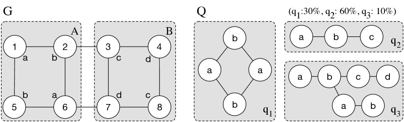
Figure 1. Example graph $G$ with query workload $\mathcal{Q}$

In specialised graph database management systems (GDBMS), pattern matching queries are highly efficient. They usually correspond to some index lookup and subsequent traversal of a small number of graph edges, where edge traversal is analogous to pointer dereferencing. However, as graphs like social networks may be both large and continually growing, eventually they saturate the memory of a single commodity machine and must be partitioned and distributed. In such a distributed setting, queries which require inter-partition traversals, such as $q_{2}$ in Fig. 1, incur network communication costs and will perform poorly. A widely recognised approach to addressing these scalability issues in graph data management is to use one of several k-way balanced graph partitioners (Huang and Abadi, 2016; Karypis and Kumar, 1997; Tsourakakis et al., 2014; Stanton and Kliot, 2012; Xu et al., 2014; Margo and Seltzer, 2015; Chevalier and Pellegrini, 2008). These systems distribute vertices, edges and queries evenly across several machines, seeking to optimise some global goal, e.g. minimising the number of edges which connect vertices in different partitions (a.k.a min. edge-cut). In so doing, they improve the performance of a broad range of possible analyses.

Whilst graphs partitioned for such global measures mostly work well for global forms of graph analysis (e.g. Pagerank), no one measure is optimal for all types of operation (Shang and Yu, 2013). In particular, the workloads of pattern matching query workloads, common to GDBMS, are a poor match for these kinds of partitioned graphs, which we call workload agnostic. This is because, intuitively, a min. edge-cut partitioning is equivalent to assuming uniform, or at least constant, likelihood of traversal for each edge throughout query processing. This assumption is unrealistic as a query workload may traverse a limited subset of edges and edge types, which is specific to its graph patterns and subject to change.

To appreciate the importance of a workload-sensitive partitioning, consider the graph of Fig.1. The partitioning $\{A,B\}$ is optimal for the balanced min. edge-cut goal, but may not be optimal for the query graphs in $Q$. For example, the query graph $q_{2}$ matches the subgraphs $\{(1,2),(2,3)\}$ and $\{(6,2),(2,3)\}$ in $G$. Given a workload which consisted entirely of $q_{2}$ queries, every one would require a potentially expensive inter-partition traversal (ipt). It is easy to see that the alternative partitioning $A^{\prime}=\{1,2,3,6\}$, $B^{\prime}=\{4,5,7,8\}$ offers an improvement (0 ipt) given such a workload, whilst being strictly worse w.r.t min. edge-cut.

Mature research of workload-sensitive online database partitioning is largely confined to relational DBMS (Quamar et al., 2013; Curino et al., 2010; Pavlo et al., 2012)

1.1. Contributions

Given the above motivation, we present Loom: a partitioner for online, dynamic graphs which optimises vertex placement to improve the performance of a given stream of sub-graph pattern matching queries.

The simple goals of Loom are threefold: a) to discover patterns of edge traversals which are common when answering queries from our given workload $Q$; b) to efficiently detect instances of these patterns in the ongoing stream of graph updates which constitutes an online graph; and c) to assign these pattern matches wholly within an individual partition or across as few partitions as possible, thereby reducing the number of ipt and increasing the average performance of any $q\in Q$.

This work extends an earlier “vision” work (Firth and Missier, 2016) by the authors, providing the following additional contributions:

• A compact  trie based encoding of the most frequent traversal patterns over edges in $G$. We show how it may be constructed and updated given an evolving workload $Q$.

• A method of sub-graph isomorphism checking, extending a recent probabilistic technique(Song et al., 2014). We show how this measure may be efficiently computed and demonstrate both the low probability of false positives and the impossibility of false negatives.

• A method for efficiently computing matches for our frequent traversal patterns in a graph stream, using our trie encoding and isomorphism method, and then assign these matching sub-graphs to graph partitions, using heuristics to preserve balance. Resulting partitions do not rely upon replication and are therefore agnostic to the complex replication schemes often used in production systems.

As online graphs are equivalent to graph streams, we present an extensive evaluation comparing Loom to popular streaming graph partitioners Fennel (Tsourakakis et al., 2014) and LDG(Stanton and Kliot, 2012). We partition real and synthetic graph streams of various sizes and with three distinct stream orderings: breadth-first, depth-first and random order. Subsequently, we execute query workloads over each graph, counting the number of expensive $ipt$ which occur. Our results indicate that Loom achieves a significant improvement over both systems, with between 15 and $40\%$ fewer $ipt$ when executing a given workload.

1.2. Related work

Partitioning graphs into k balanced subgraphs is clearly of practical importance to any application with large amounts of graph structured data. As a result, despite the fact that the problem is known to be NP-Hard (Andreev and Racke, 2006), many different solutions have been proposed (Huang and Abadi, 2016; Karypis and Kumar, 1997; Tsourakakis et al., 2014; Stanton and Kliot, 2012; Xu et al., 2014; Margo and Seltzer, 2015; Chevalier and Pellegrini, 2008). We classify these partitioning approaches into one of three potentially overlapping categories: streaming, non-streaming and workload sensitive. Loom is both a streaming and workload-sensitive partitioner.

Non-streaming graph partitioners (Karypis and Kumar, 1997; Chevalier and Pellegrini, 2008; Margo and Seltzer, 2015) typically seek to optimise an objective function global to the graph, e.g. minimising the number of edges which connect vertices in different partitions (min. edge-cut).

A common class of these techniques is known as multi-level partitioners (Karypis and Kumar, 1997; Chevalier and Pellegrini, 2008). These partitioners work by computing a succession of recursively compressed graphs, tracking exactly how the graph was compressed at each step, then trivially partitioning the smallest graph with some existing technique. Using the knowledge of how each compressed graph was produced from the previous one, this initial partitioning is then “projected” back onto the original graph, using a local refinement technique (such as Kernighan-Lin (Kernighan and Lin, 1970)) to improve the partitioning after each step. A well known example of a multilevel partitioner is METIS (Karypis and Kumar, 1997), which is able to produce high quality partitionings for small and medium graphs, but performance suffers significantly in the presence of large graphs (Tsourakakis et al., 2014). Other mutlilevel techniques (Chevalier and Pellegrini, 2008) share broadly similar properties and performance, though they differ in the method used to compress the graph being partitioned.

Other types of non-streaming partitioner include Sheep (Margo and Seltzer, 2015): a graph partitioner which creates an elimination tree from a distributed graph using a map-reduce procedure, then partitions the tree and subsequently translates it into a partitioning of the original graph. Sheep optimises for another global objective function: minimising the number of different partitions in which a given vertex $v$ has neighbours (min. communication volume).

These non-streaming graph partitioners suffer from two main drawbacks. Firstly, due to their computational complexity and high memory usage(Stanton and Kliot, 2012), they are only suitable as offline operations, typically performed ahead of analytical workloads. Even those partitioners which are distributed to improve scalability, such as Sheep or the parallel implementation of Metis (ParMetis) (Karypis and Kumar, 1997), make strong assumptions about the availability of global graph information. As a result they may require periodic re-execution, i.e. given a dynamic graph following a series of graph updates, which is impractical online (Jindal and Dittrich, 2012). Secondly, as mentioned, partitioners which optimise for such global measures assume uniform and constant usage of a graph, causing them to “leave performance on the table” for many workloads.

Streaming graph partitioners (Tsourakakis et al., 2014; Stanton and Kliot, 2012; Huang and Abadi, 2016) have been proposed to address some of the problems with partitioners outlined above. Firstly, the strict streaming model considers each element of a graph stream as it arrives, efficiently assigning it to a partition. Additionally, streaming partitioners do not perform any refinement, i.e. later reassigning graph elements to other partitions, nor do they perform any sort of global introspection, such as spectral analysis. As a result, the memory usage of streaming partitioners is both low and independent of the size of the graph being partitioned, allowing streaming partitioners to scale to to very large graphs (e.g. billions of edges). Secondly, streaming partitioners may trivially be applied to continuously growing graphs, where each new edge or update is an element in the stream.

Streaming partitioners, such as Fennel (Tsourakakis et al., 2014) and LDG (Stanton and Kliot, 2012), make partition assignment decisions on the basis of inexpensive heuristics which consider the local neighbourhood of each new element at the time it arrives. For instance, LDG assigns vertices to the partitions where they have the most neighbours, but penalises that number of neighbours for each partition by how full it is, maintaining balance. By using the local neighbourhood of a graph element $e$ at the time $\mathbf{e}$ is added, such heuristics render themselves sensitive to the ordering of a graph stream. For example, a graph which is streamed in the order of a breadth-first traversal of its edges will produce a better quality partitioning than a graph which is streamed in random order, which has been shown to be pseudo adversarial(Tsourakakis et al., 2014).

In general, streaming algorithms produce partitionings of lower quality than their non-streaming counterparts but with much improved performance. However, some systems, such as the graph partitioner Leopard (Huang and Abadi, 2016), attempt to strike a balance between the two. Leopard relies upon a streaming algorithm (Fennel) for the initial placement of vertices but drops the “one-pass” requirement and repeatedly considers vertices for reassignment; improving quality over time for dynamic graphs, but at the cost of some scalability. Note that these Streaming partitioners, like their non-streaming counterparts, are workload agnostic and so share those disadvantages.

Workload sensitive partitioners (Peng et al., 2016; Xu et al., 2014; Shang and Yu, 2013; Curino et al., 2010; Quamar et al., 2013; Pavlo et al., 2012) attempt to optimise the placement of data to suit a particular workload. Such systems may be streaming or non-streaming, but are discussed separately here because they pertain most closely to the work we do with Loom.

Some partitioners, such as LogGP (Xu et al., 2014) and CatchW (Shang and Yu, 2013), are focused on improving graph analytical workloads designed for the bulk synchronous parallel (BSP) model of computation. In the BSP model a graph processing job is performed in a number of supersteps, synchronised between partitions. CatchW examines several common categories of graph analytical workload and proposes techniques for predicting the set of edges likely to be traversed in the next superstep, given the category of workload and edges traversed in the previous one. CatchW then moves a small number of these predicted edges between supersteps, minimising inter-partition communication. LogGP uses a similar log of activity from previous supersteps to construct a hypergraph where vertices which are frequently accessed together are connected. LogGP then partitions this hypergraph to suggest placement of vertices, reducing the analytical job’s execution time in future.

In the domain of RDF stores, Peng et al. (Peng et al., 2016) use frequent sub-graph mining ahead of time to select a set of patterns common to a provided SPARQL query workload. They then propose partitioning strategies which ensure that any data matching one of these frequent patterns is allocated wholly within a single partition, thus reducing average query response time at the cost of having to replicate (potentially many) sub-graphs which form part of multiple frequent patterns.

For RDBMS, systems such as Schism (Curino et al., 2010) and SWORD (Quamar et al., 2013) capture query workload samples ahead of time, modelling them as hypergraphs where edges correspond to sets of records which are involved in the same transaction. These graphs are then partitioned using existing non-streaming techniques (METIS) to achieve a min. edge-cut. When mapped back to the original database, this partitioning represents an arrangement of records which causes a minimal number of transactions in the captured workload to be distributed. Other systems, such as Horticulture (Pavlo et al., 2012), rely upon a function to estimate the cost of executing a sample workload over a database and subsequently explore a large space of possible candidate partitionings. In addition to a high upfront cost (Curino et al., 2010; Pavlo et al., 2012), these techniques focus on the relational data model, and so make simplifying assupmtions, such as ignoring queries which traverse $>1$-2 edges (Quamar et al., 2013) (i.e. which perform nested joins). Larger traversals are common to sub-graph pattern matching queries, therefore its unclear how these techniques would perform given such a workload.

Overall, the works reviewed above either focus on different types of workload than we do with Loom (namely offline analytical or relational queries), or they make extensive use of replication. Loom does not use any form of replication, both to avoid potentially significant storage overheads (Pujol et al., 2010) and to remain interoperable with the sophisticated replication schemes used in production systems.

1.3. Definitions

Here we review and define important concepts used throughout the rest of the paper.

A labelled graph $G=(V,E,L_{V},f_{l})$ is of the form: a set of vertices $V=\{v_{1},v_{2},...,v_{n}\}$, a set of pairwise relationships called edges $e=(v_{i},v_{j})\in E$ and a set of vertex labels $L_{V}$. The function $f_{\mathit{l}}:V\rightarrow L_{V}$ is a surjective mapping of vertices to labels. We view an online graph simply as a (possibly infinite) sequence of edges which are being added to a graph $G$, over time. We consider fixed width sliding windows over such a graph, i.e. a sliding window of time $t$ is equivalent to the $t$ most recently added edges. Note that an online may be viewed as a graph stream and we use the two terms interchangeably.

A pattern matching query is defined in terms of sub-graph isomorphism. Given a pattern graph $q=(V_{q},E_{q})$, a query should return $R$: a set of sub-graphs of $G$. For each returned sub-graph $R_{i}=(V_{R_{i}},E_{R_{i}})$ there should exist a bijective function $f$ such that: a) for every vertex $v\in V_{R_{i}}$, there exists a corresponding vertex $f(v)\in V_{q}$; b) for every edge $(v_{1},v_{2})\in E_{R_{i}}$, there exists a corresponding edge $(f(v_{1}),f(v_{2}))\in E_{q}$; and c) for every vertex $v\in R_{i}$, the labels match those of the corresponding vertices in $q$, $l(v)=l(f(v))$. A query workload is simply a multiset of these queries $Q=\{(q_{1},n_{1})\ldots(q_{h},n_{h})\}$, where $n_{i}$ is the relative frequency of $q_{i}$ in $Q$.

A query motif is a graph which occurs, with a frequency of more than some user defined threshold $\mathcal{T}$, as a sub-graph of query graphs from a workload $Q$.

A vertex centric graph partitioning is defined as a disjoint family of sets of vertices $P_{k}(G)=\{V_{1},V_{2},\ldots,V_{k}\}$. Each set $V_{i}$, together with its edges $E_{i}$ (where $e_{i}\in E_{i}$, $e_{i}=(v_{i},v_{j})$, and $\{v_{i},v_{j}\}\subseteq V_{i}$), is referred to as a partition $S_{i}$. A partition forms a proper sub-graph of $G$ such that $S_{i}=(V_{i},E_{i})$, $V_{i}\subseteq V$ and $E_{i}\subseteq E$. We define the quality of a graph partitioning relative to a given workload $Q$. Specifically, the number of inter-partition traversals ($ipt$) which occur while executing $Q$ over $P_{k}(G)$. Whilst min. edge-cut is the standard scale free measure of partition quality (Karypis and Kumar, 1997), it is intuitively a proxy for $ipt$ and, as we have argued (Sec. 1), not always an effective one.

1.4. Overview

Once again, Loom continuously partitions an online graph $G$ into $k$ parts, optimising for a given workload $Q$. The resulting partitioning $P_{k}(G,Q)$ reduces the probability of expensive $ipt$, when executing a random $q\in Q$, using the following techniques.

Firstly, we employ a trie-like datastructure to index all of the possible sub-graphs of query graphs $q\in Q$, then identify those sub-graphs which are motifs, i.e. occur most frequently (Sec. 2). Secondly, we buffer a sliding window over $G$, then use an efficient graph stream pattern matching procedure to check whether each new edge added to $G$ creates a sub-graph which matches one of our motifs (Sec. 3). Finally, we employ a combination of novel and existing partitioning heuristics to assign each motif matching sub-graph which leaves the sliding window entirely within an individual partition, thereby reducing $ipt$ for $Q$ (Sec. 4).

2. Identifying Motifs

We now describe the first of the three steps mentioned above, namely the encoding of all query graphs found in our pattern matching query workload $Q$. For this, we use a trie-like datastructure which we have called the Traversal Pattern Summary Trie (TPSTry++). In a TPSTry++, every node represents a graph, while every parent node represents a sub-graph which is common to the graphs represented by its children. As an illustration, the complete TPSTry++ for the workload $Q$ in Fig. 1 is shown in Fig. 2.

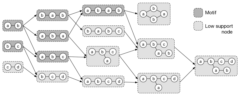
Figure 2. TPSTry++ for $\mathcal{Q}$ in fig. 1

This structure not only encodes all sub-graphs found in each $q\in Q$, it also associates a support value $p$ with each of its nodes, to keep track of the relative frequency of occurrences of each sub-graph in our query graphs.

Given a threshold $\mathcal{T}$ for the frequency of occurrences, a motif is a sub-graph that occurs at least $\mathcal{T}$ times in $Q$. As an example, for $\mathcal{T}=40\%$, $Q$’s motifs are the shaded nodes in Fig. 2.

Intuitively, a sub-graph of $G$ which is frequently traversed by a query workload should be assigned to a single partition. We can idenfity these sub-graphs as they form within the stream of graph updates, by matching them against the motifs in the TPSTry++. Details of the motif matching process are provided in Sec.3. In the rest of this section we explain how a TPSTry++ is constructed, given a workload $Q$.

A TPSTry++ extends a simpler structure, called TPSTry, which we have recently proposed in a similar setting (Firth and Missier, 2017). It employs frequent sub-graph mining(Jiang et al., 2004) to compactly encode general labelled graphs. The resulting structure is a Directed Acyclic Graph (DAG), to reflect the multiple ways in which a particular query pattern may extend shorter patterns. For example in Fig. 2 the graph in node $a$-$b$-$a$-$b$ can be produced in two ways, by adding a single $a$-$b$ edge to either of the sub-graphs $b$-$a$-$b$, and $a$-$b$-$a$. In contrast, a TPSTry is a tree that encodes the space of possible traversal paths through a graph as a conventional trie of strings, where a path is a string of vertex labels, and possible paths are described by a stream of regular path queries (Mendelzon and Wood, 1995).

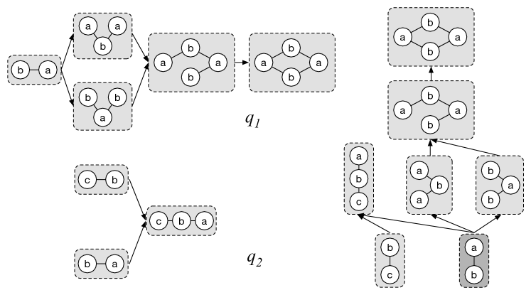
Figure 3. Combining tries for query graphs $q_{1}$, $q_{2}$

Note that the trie is a relatively compact structure, as it grows with $|L_{V}|^{t}$, where $t$ is the number of edges in the largest query graph in $Q$ and $L_{V}$ is typically small. Also note that the TPSTry++ is similar to, though more general than, Ribiero et al’s G-Trie (Ribeiro and Silva, 2014) and Choudhury et al’s SJ-Tree (Choudhury et al., 2015), which use trees (not DAGs) to encode unlabelled graphs and labelled paths respectively.

2.1. Sub-graph signatures

We build the trie for $Q$ by progressively building and merging smaller tries for each $q\in Q$, as shown in Fig. 3. This process relies on detecting graph isomorphisms, as any two trie nodes from different queries that contain identical graphs should be merged. Failing to detect isomorphism would result, for instance, in two separate trie nodes being created for the simple graphs $a$-$b$-$c$ and $c$-$b$-$a$, rather than a single node with a support of 2, as intended. One way of detecting isomorphism, often employed in frequent sub-graph mining, involves computing the lexicographical canonical form for each graph (McKay, 1981), whereby two graphs are isomorphic if and only if they have the same canonical representation.

Computing a graph’s canonical form provides strong guarantees, but can be expensive(Ribeiro and Silva, 2014). Instead, we propose a probabilistic, but computationally more efficient approach based on number theoretic signatures, which extends recent work by Song et al. (Song et al., 2014). In this approach we compute the signature of a graph as a large, pseudo-unique integer hash that encodes key information such as its vertices, labels, and nodes degree. Graphs with matching signatures are likely to be isomorphic to one another, but there is a small probability of collision, i.e., of having two different graphs with the same signature.

Given a query graph $G_{q}=\{V_{q},E_{q}\}$ we compute its signature as follows. Initially we assign a random value $r(l)=[1,p)$, between 1 and some user specified prime $p$, to each possible label $l\in L_{V_{i}}$ from our data graph $G$; recall that the function $f_{\mathit{l}}$ maps vertices in $G$ to these labels. We then perform three steps:

1. Calculate a factor for each edge $e=(v_{i},v_{j})\in E_{q}$, according to the formula:

   $$edgeFac(e)=(r(f_{\mathit{l}}{}(v_{i}))-r(f_{\mathit{l}}{}(v_{j})))\ mod\ p$$

2. Calculate the factors that encode the degree of each vertex. If a vertex $v$ has a degree $n$, its degree factor is defined as:

   $$degFac(v)=((r(f_{\mathit{l}}{}(v))+1)\ mod\ p)\cdot$$

   $$((r(f_{\mathit{l}}{}(v ))+2)\ mod\ p)\cdot\ldots\cdot((r(f_{\mathit{l}}{}(v))+n)\ mod\ p)$$

3. Finally, we compute the signature of $G_{q}=(V_{q},E_{q})$ as:

   $$(\prod_{e\in E_{i}}edgeFac(e))\cdot{}(\prod_{v\in V_{i}}degFac(v))$$

To illustrate, consider query $q_{1}$ from Fig. 1. Given a $p$ of 11 and random values $r(a)=3$, $r(b)=10$ we first calculate the edge factor for an $a$-$b$ edge: $edgeFac((a,b))=(3-10)\ mod\ 11=7$. As $q_{1}$ consists of four $a$-$b$ edges, its total edge factor is $7^{4}=2401$. Then we calculate the degree factors , starting with a $b$ labelled vertex with degree 2: $degFac(b)=((10+1)\ mod\ 11)\cdot((10+2)\ mod\ 11)=11$, followed by an $a$ labelled vertex also with degree 2: $degFac(a)=20$. As there are two of each vertex, with the same degree, the total degree factor is $11^{2}\cdot 20^{2}=48400$. The signature of $q_{1}=2401\cdot 48400=116208400$.

This approach is appealing for two reasons. Firstly, since the factors in the signature may be multiplied in any order, a signature for $G$ can be calculated incrementally if the signature of any of its sub-graphs $G_{i}$ is known, as this is the combined factor due to the additional edges and degree in $G\setminus G_{i}$. Secondly, the choice of $p$ determines a trade-off between the probability of collisions and the performance of computing signatures. Specifically, note that signatures can be very large numbers (thousands of bits) even for small graphs, rendering operations such as remainder costly and slow. A small choice of $p$ reduces signature size, because all the factors are mapped to a finite field (Lidl and Niederreiter, 1997) (factor mod p) between 1 and $p$, but it increases the likelihood of collision, i.e., the probability of two unrelated factors being equal. We discuss how to improve the performance and accuracy of signatures in Section 2.3.

2.2. Constructing the TPSTry++

Algorithm 1 Recursively add a query graph $G_{q}$ to a TPSTry++

1:  $factors(e,g)\leftarrow$ degree/edge factors to multiply a graph $g$’s signature when adding edge $e$

2:  $support(g)\leftarrow$ a map of TPSTry++ nodes (graphs) to $p$-values

3:  $tpstry\leftarrow$ the TPSTry++ for workload $\mathcal{Q}$

4:  $parent\leftarrow$ a TPSTry++ node, initially root (an empty graph)

5:  $G_{q}\leftarrow$ the query graph defined by a query $q$

6:  $g$ some sub-graph of $G_{q}$

7:  $\mathbf{for}$ $e$ in edges from $G_{q}$ $\mathbf{do}$

8:      $\mathbf{g}\leftarrow$ new empty graph

9:      $\mathbf{corecurse(parent,e,tpstry,g)}$

10:          $sig\leftarrow factor(e,g)\cdot parent.signature$

11:          $\mathbf{if}$ $tpstry.signatures$ contains $sig$ $\mathbf{then}$

12:             $n\leftarrow$ node from $tpstry$ with signature $sig$

13:             $n.support\leftarrow$ $n.support+1$

14:          $\mathbf{else}$

15:             $n\leftarrow$ new node with graph $g+e$, signature $sig$ and support 1

16:             $tpstry\leftarrow tpstry+n$

17:          $\mathbf{if~{}not}$ $parent.children$ contains $n$ $\mathbf{then}$

18:             $parent.children\leftarrow$ $parent.children+n$

19:          $newEdges\leftarrow$ edges incident to $g+e$ & not in $g+e$

20:          $\mathbf{for}$ $e^{\prime}$ in $newEdges$

21:             $\mathbf{corecurse(n,e^{\prime},tpstry,g+e)}$

22:  $\mathbf{return}$ $tpstry$

Our approach to constructing the TPSTry++ is to incrementally compute signatures for sub-graphs of each query graph $q$ in a trie, merging trie nodes with equal signatures to produce a DAG which encodes the sub-graphs of all $q\in Q$. Alg. 1 formalises this approach.

Essentially, we recursively “rebuild” the graph $G_{q}$ $\mid Eq\mid$ times, starting from each edge $e\in E_{q}$ in turn. For an edge $e$ we calculate its edge and degree factors, initially assuming a degree of 1 for each vertex. If the resulting signature is not associated with a child of the TPSTry++’s root, then we add a node $n$ representing $e$. Subsequently, we “add” those edges $e^{\prime}$ which are incident to $e\in G_{q}$, calculating the additional edge and degree factors, and add corresponding trie nodes as children of $n$. Then we recurse on the edges incident $e+e^{\prime}$.

Consider again our earlier example of the query graph $q_{1}$: as it arrives in the workload stream $Q$, we break it down to its constituent edges {a-b, a-b, a-b, a-b}. Choosing an edge at random we calculate its combined factor. We know that the edge factor of an $a$-$b$ edge is 7. When considering this single edge, both $a$ and $b$ vertices have a degree of 1, therefore the signature for $a$-$b$ is $7\cdot((3+1)\ mod\ 11)\cdot((10+1)\ mod\ 11)=308$. Subsquently, we do the same for all other edges and, finding that they have the same signature, leave the trie unmodified. Next, for each edge, we add each incident edge from $q_{1}$ and compute the new combined signature. Assume we add another $a$-$b$ edge adjacent to $b$ to produce the sub-graph $a$-$b$-$a$. This produces three new factors: the new edge factor $7$, the new $a$ vertex degree factor $((3+1)\ mod\ 11)$ and an additional degree factor for the existing $b$ vertex $((10+2)\ mod\ 11)$. The combined signature for $a$-$b$-$a$ is therefore $308\cdot 7\cdot 4\cdot 1=8624$; if a node with this signature does not exist in the trie as a child of the $a$-$b$ node, we add it. This continues recursively, considering larger sub-graphs of $q_{1}$ until there are no edges left in $q_{1}$ which are not in the sub-graph, at which point, $q_{1}$ has been added to the TPSTry++.

2.3. Avoiding signature collisions

As mentioned, number theoretic signatures are a probabilistic method of ismorphism checking, prone to collisions. There are several scenarios in which two non-isomorphic graphs may have the same signature: a) two factors representing different graph features, such as different edges or vertex degrees, are equal; b) two distinct sets of factors have the same product; and c) two different graphs have identical sets of edges, vertices and vertex degrees.

The original approach to graph isomorphic checking (Song et al., 2014) makes use of an expensive authoritative pattern matching method to verify identified matches. Given a query graph, it calculates its signature in advance, then incrementally computes signatures for sub-graphs which form within a window over a graph stream. If a sub-graph’s signature is ever divisible by that of the query graph, then that sub-graph should contain a query match.

There are some key differences in how we compute and use signatures with Loom, which allow us to rely solely upon signatures as an efficient means for mining and matching motifs. Firstly, remember our overall aim is to heuristically lower the probability that sub-graphs in a graph $G$ which match our discovered motifs straddle a partition boundary. As a result we can tolerate some small probability of false positive results, whilst the manner in which signatures are executed (Sec. 2.1) precludes false negatives; i.e. two graphs which are isomorphic are guaranteed to have the same signature. Secondly, we can exploit the structure of the TPSTry++ to avoid ever explicitly computing graph signatures. From Fig. 2 and Alg. 1, we can see that all possible sub-graphs of a query graph $G_{q}$ will exist in the TPSTry++ by construction. We calculate the edge and degree factors which would multiply the signature of a sub-graph with the addition of each edge, then associate these factors to the relevant trie branches. This allows us to represent signatures as sets of their constituent factors, which eliminates a source of collisions, e.g. we can now distinguish between graphs with factors $\{6,2\}$, $\{4,3\}$ and $\{12\}$. Thirdly, we never attempt to discover whether some sub-graph contains a match for query $q$, only whether it is a match for $q$. In other words, the largest graph for which we calculate a signature is the size of the largest query graph $|G_{q}|$ for all $q\in Q$, which is typically small. This allows us to choose a larger prime $p$ than Song et al. might, as we are less concerned with signature size, reducing the probability of factor collision, another source of false positive signature matches.

Concretely, we wish to select a value of $p$ which minimises the probability that more than some acceptable percentage $\mathcal{C}\%$ of a signature’s factors are collisions. From Section 2.1 there are three scenarios in which a factor collision may occur: a) two edge factors are equal despite different vertices with different random values from our range $[1,p)$; b) an edge factor is equal to a degree factor; and c) two degree factors are equal, again despite different vertices. Song et al. show that all factors are uniform random variables from $[1,p)$, therefore each scenario occurs with probability $\frac{1}{p}$.

For either edge or degree factors, from the above it is clear that there are two scenarios in which a collision may occur, giving a collision probability for any given factor of $\frac{2}{p}$. The Handshaking lemma tells us that the total degree of a graph must equal $2|E|$, which means that a graph must have $3|E|$ factors in its signature: one per edge plus one per degree. Combined with the binary measure of “success” (collision / no collision), this suggests a binomial distribution of factor collision probabilities, specifically $Binomial(3|E|,\frac{2}{p})$. Binomial distributions tell us the probability of exactly $x$ “successes” occuring, however we want the probability that no more than $\mathcal{C}_{max}=\mathcal{C}\%\cdot 3|E|$ factors collide and so must sum over all acceptable outcomes $x\in\mathcal{C}_{max}$:

$$\sum_{x=0}^{\mathcal{C}_{max}}Pr(X=x)\text{ where }X\sim Binomial(3|E|,\frac{2}{p})$$

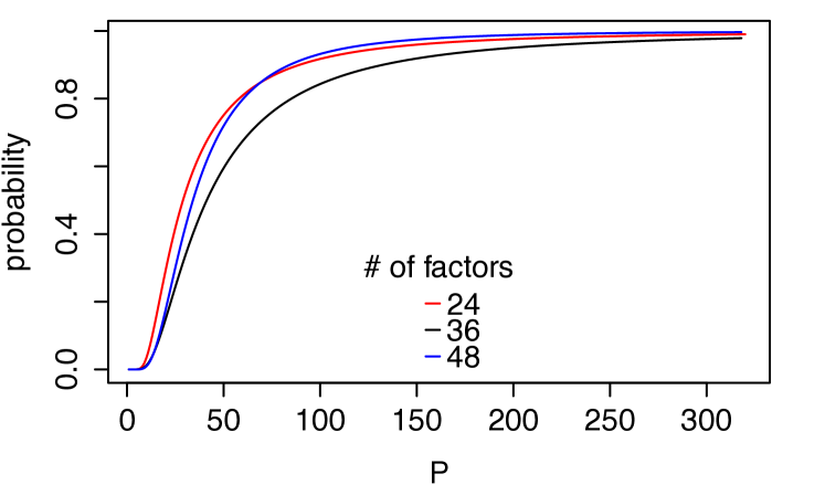
Figure 4. Probability of $<5\%$ factor collisions for various $p$

Figure 4 shows the probabilities of having fewer than $5\%$ factor collisions given query graphs of 8, 12 or 16 edges and $p$ choices between 2 and 317. In Loom, when identifying and matching motifs, we use a $p$ value of 251, which as you can see gives a neglible probability of significant factor collisions.

3. Matching Motifs

We have seen how motifs that occur in $Q$ are identified. By construction, motifs represent graph patterns that are frequently traversed during executions of queries in $Q$. Thus, the sub-graphs of $G$ that match those motifs are expected to be frequently visited together and are therefore best placed within the same partition. In this section we clarify how we discover pattern matches between sub-graphs and motifs, whilst in the next Section we describe the allocation of those sub-graphs to partitions.

Loom operates on a sliding window of configurable size over the stream of edges that make up the growing graph $G$. The system monitors the connected sub-graphs that form in the stream within the space of the window, efficiently checking for isomorphisms with any known motif each time a sub-graph grows. Upon leaving the window, sub-graphs that match a motif are immediately assigned to a partition, subject to partition balance constraints as explained in Section 4.

Note that this technique introduces a delay, corresponding to the size of the window, between the time edges are submitted to the system and the time they are assigned and made available. In order to allow queries to access the new parts of graph $G$, Loom views the sliding window itself as an extra partition, which we denote $P_{temp}$. In practice, vertices and edges in the window are accessible in this temporary partition prior to being permanently allocated to their own partition.

To help understand how the matching occurs, note that in the TPSTry++, by construction, all anscestors of any node $n$ must represent strict sub-graphs of the graph represented by $n$ itself. Also, note that the support of a node $n$ is the relative frequency with which $n$’s sub-graph $G_{n}$ occurs in $Q$. As, by definition, each time $G_{n}$ occurs in $Q$ so do all of its sub-graphs, a trie node $n$ must have a support lower than any of its anscestors. This means that if any of the nodes in the trie, including those representing single edges, are not motifs, then none of their descendants can be motifs either. Thus, when a new edge $e=(v_{1},v_{2})$ arrives in the graph stream, we compute its signature (Sec. 2.1) and check if $e$ matches a single-edge motif at the root of the TPSTry++. If there is no match, we can be certain that $e$ will never form part of any sub-graph that matches a motif. We therefore immediately assign $e$ to a partition and do not add it to our stream window $P_{temp}$. If, on the other hand, $e$ does match a single-edge motif then we record the match into a map, matchList, and add $e$ to the window. The matchList maps vertices $v$ to the set of motif matching sub-graphs in $P_{temp}$ which contain $v$; i.e. having determined that $e=(v_{1},v_{2})$ is a motif match, we treat $e$ as a sub-graph of a single edge, then add it to the matchList entries for both $v_{1}$ and $v_{2}$. Additionally, alongside every sub-graph in matchList, we store a reference to the TPSTry++ node which represents the matching motif. Therefore, entries in matchList take the form $v\rightarrow\{\langle E_{i},m_{i}\rangle,\langle E_{j},m_{j}\rangle,\ldots\}$, where $E_{i}$ is a set of edges in $P_{temp}$ that form a sub-graph $g_{i}$ with the same signature as the motif $m_{i}$.

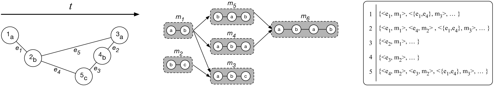
Figure 5. $t$-length window over $G$ (left), Motifs from TPSTry++ (center) and motif $matchList$ for window (right)

Given the above, any edge $e$ which is added to $P_{temp}$ must at least match a single edge motif. However, if $e$ is incident to other edges already in $P_{temp}$, then its addition may also form larger motif matching sub-graphs which we must also detect and add to matchList. Thus, having added $e=(v_{1},v_{2})$ to matchList, we check the map for existing matches which are connected to $e$; i.e we look for matches which contain one of $v_{1}$ or $v_{2}$. If any exist, we use the procedure in Alg. 2, along with the TPSTry++, to determine whether the addition of edge $e$ to these sub-graphs creates another motif match.

Essentially, for each sub-graph $g_{i}$ from matchList to which $e$ is connected, we calculate the set of edge and degree factors $fac(e,g_{i})$ which would multiply the signature of $g_{i}$ upon the addition $e$, as in Sec. 2. Recall, also from Sec. 2, that a TPSTry++ node contains a signature for the graph it represents, and that these signatures are stored as sets of factors, rather than their large integer products. As each sub-graph in matchList is paired with its associated motif $n$ from the trie, we can efficiently check if $n$ has a child $c$ where a) $c$ is a motif; and b) the difference between $n$’s factor set and $c$’s factor set corresponds to factors for the addition of $e$ to $g_{i}$, i.e., $fac(e,g_{i})=c.signatures\setminus n.signatures$.

Algorithm 2 Mine motif matches from each new edge $e\in G$

1:  $fac(e,g)\leftarrow$ degree/edge factors to multiply a graph $g$’s signature when adding edge $e$

2:  $tpstry\leftarrow$ the filtered TPSTry++ of motifs for workload $Q$

3:  $\mathbf{for}$ each new edge $e(v_{1},v_{2})$ $\mathbf{do}$

4:      $matches\leftarrow matchList(v_{1})\cup matchList(v_{2})$

5:      $\mathbf{for}$ each sub-graph $m$ in $matches$ $\mathbf{do}$

6:         $n\leftarrow$ the $tpstry$ node for $m$

7:         $\mathbf{if}$ $n$ has child $c$ w. $factor=fac(e,m)$ $\mathbf{then}$

8:           add $\langle m+e,c\rangle$ to $matchList$ for $v_{1}\&v_{2}$ //Match found!

9:      $ms_{1}\leftarrow matchList(v_{1})$

10:      $ms_{2}\leftarrow matchList(v_{2})$

11:      $\mathbf{for}$ all possible pairs $(m_{1},m_{2})$ from $(ms_{1},ms_{2})$ $\mathbf{do}$

12:         $n_{1}\leftarrow$ the $tpstry$ node for $m_{1}$

13:         $\mathbf{recurse(tpstry,m_{2},m_{1},n_{1})}$

14:           $\mathbf{for}$ each edge $e_{2}$ in $m_{2}$ $\mathbf{do}$

15:              $\mathbf{if}$ $n_{1}$ has child $c_{1}$ w. $factor=fac(e_{2},m_{1})$ $\mathbf{then}$

16:                 $\mathbf{recurse(tpstry,m_{2}-e_{2},m_{1}+e_{2},c_{1})}$

17:           $\mathbf{if}$ $m_{2}$ is empty $\mathbf{then}$ //Match found!

18:              add $\langle m_{1}+m_{2},n_{1}\rangle$ to $matchList$ for $v_{1}\&v_{2}$

If such a child exists in the trie then adding $e$ to a graph which matches motif $n$ ($g_{i}$) will likely create a graph which matches motif $c$: the addition of $e$ to $P_{temp}$ has formed the new motif matching sub-graph $g_{i}+e$.

We also detect if the joining of two existing multi edge motif matches $(\langle E_{1},m_{1}\rangle,\langle E_{2},m_{2}\rangle)$ forms yet another motif match, in roughly the same manner. First we consider each edge from the smaller motif match (e.g. $e\in E_{2}$ from $\langle E_{2},m_{2}\rangle$), checking if the addition of any of these edges to $E_{1}$ constitutes yet another match; if it does then we add the edge to $E_{1}$ and recursively repeat the process until $E_{2}$ is empty. If this process does exhaust $E_{2}$ then $E_{1}\cup E_{2}$ constitute a motif matching sub-graph. Once this process is complete, matchList will contain entries for all of the motif matching sub-graphs currently in $P_{temp}$. Note that as more edges are added to $P_{temp}$, matchList may contain multiple entries for a given vertex where one match is a sub-graph of another, i.e. new motif matches don’t replace existing ones.

As an example of the motif matching process, consider the portion of a graph stream (left), motifs (center) and matchList (right) depicted in Fig. 5. Our window over the graph stream $G$ is initially empty, with the depicted edges being added in label order (i.e. $e_{1},e_{2},\ldots$). As the edge $e_{1}$ is added, we first compute its signature and verify whether $e_{1}$ matches a single-edge motif in the TPSTry++. We can see that, as an $a$-$b$ labelled edge, the signature for $e_{1}$ must match that of motif $m_{1}$, therefore we add $e_{1}$ to $P_{temp}$, and add the entry $\langle e_{1},m_{1}\rangle$ to matchList for both $e_{1}$’s vertices 1,2. As $e_{1}$ is not yet connected to any other edges in $P_{temp}$, we do not need to check for the formation of additional motif matches. Subsequently, we perform the exact same process for edge $e_{2}$. When $e_{3}$ is added, again we verify that, as a $b$-$c$ edge, $e_{3}$ is a match for the single-edge motif $m_{3}$ and so update $P_{temp}$ and matchList accordingly. However, $e_{3}$ is connected to existing motif matching sub-graphs in $P_{temp}$ therefore the union of matchList entries for $e_{3}$’s vertices 4,5 (line 4 Alg. 2) returns $\{\langle e_{2},m_{1}\rangle\}$. As a result, we calculate the factors to multiply $e_{2}$’s signature by, when adding $e_{3}$. Remember that when computing signatures, each edge has a factor, as well as each degree. Thus, when adding $e_{3}$ to $e_{2}$ our new factors are an edge factor for a $b$-$c$ labelled edge, a first degree factor for the vertex labelled $c$ (5) and a second degree factor for the vertex labelled $b$ (4) (Sec. 2.1). Subsquently we must check whether the motif for $e_{2}$, $m_{1}$, has any child nodes with additional factors consistent with the addition of a $b$-$c$ edge, which it does: $m_{3}$. This means we have found a new sub-graph in $P_{temp}$ which matches the motif $m_{3}$, and must add $\langle\{e_{2},e_{3}\},m_{3}\rangle$ to the matchList entries for vertices 3, 4 and 5. Similarly, the addition of $b$-$c$ labelled edge $e_{4}$ to our graph stream produces the new motif matches $\langle e_{4},m_{2}\rangle$ and $\langle\{e_{1},e_{4}\},m_{3}\rangle$, as can be seen in our example matchList.

Finally, the addition of our last edge, $e_{5}$, creates several new motif matches (e.g. $\langle\{e_{1},e_{5}\},m_{4}\rangle,\langle\{e_{2},e_{5}\},m_{5}\rangle$ etc…). In particular, notice that the addition of $e_{5}$ creates a match for the motif $m_{6}$, combining the new motif match $\langle\{e_{1},e_{5}\},m_{4}\rangle$ with an existing one $\langle e_{2},m_{1}\rangle$. To understand how we discover these slightly more complex motif matches, consider Alg. 2 from line 11 onwards. First we retrieve the updated matchList entries for vertices 2 and 3, including the new motif matches gained by simply adding the single edge $e_{5}$ to connected existing motif matches, as above. Next we iterate through all possible pairs of motif matches for both vertices. Given the pair of matches $(\langle\{e_{1},e_{5}\},m_{4}\rangle,\langle e_{2},m_{1}\rangle)$, we discover that the addition of any edge from the smaller match (i.e. $e_{2}$) to the larger produces factors which correspond to a child of $m_{4}$ in the TPSTry++: $m_{6}$. As $e_{2}$ is the only edge in the smaller match, we simply add the match $\langle\{e_{1},e_{2},e_{5}\},m_{6}\rangle$ to the matchList entries for 1, 2, 3 and 4. In the general case however, we would not add this new match but instead recursively “grow” it with new edges from the smaller match, updating matchList only if all edges from the smaller match have been successfully added.

4. Allocating Motifs

Following graph stream pattern matching, we are left with a collection of sub-graphs, consisting solely of the most recent $t$ edges in $G$, which match motifs from $Q$. As new edges arrive in the graph stream, our window $P_{temp}$ grows to size $t$ and then “slides”, i.e. each new edge added to a full window causes the oldest ($t+1^{th}$) edge $e$ to be dropped. Our strategy with Loom is to then assign this old edge $e$ to a permanent partition, along with the other edges in the window which form motif matching sub-graphs with $e$. The sole exception to this is when an edge arrives that may not form part of any motif match and is assigned to a partition immediately (Sec. 3). This exception does not pose a problem however, because Loom behaves as if the edge was never added to the window and therefore does not cause displacement of older edges.

Recall again that with Loom we are attempting to assign motif matching sub-graphs wholly within individual partitions with the aim of reducing $ipt$ when executing our query workload $Q$. One naive approach to achieving this goal is as follows: When assigning an edge $e=(v_{1},v_{2})$, retrieve the motif matches associated with $v_{1}$ and $v_{2}$ from $P_{temp}$ using our $matchList$ map, then select the subset $M_{e}$ that contains $e$, where $M_{e}=\{\langle E_{1},m_{1}\rangle,\ldots\langle E_{n},m_{n}\rangle\}$, $e\in E_{i}$ and $E_{i}$ is a match for $m_{i}$. Finally, treating these matches as a single sub-graph, assign them to the partition which they share the most incident edges. This approach would greedily ensure that no edges belonging to motif matching sub-graphs in $G$ ever cross a partition boundary. However, it would likely also have the effect of creating highly unbalanced partition sizes, portentially straining the resources of a single machine, which prompted partitioning in the first place.

Instead, we rely upon two distinct heuristics for edge assignment, both of which are aware of partition balance. Firstly, for the case of non-motif-matching edges that are assigned immediately, we use the existing Linear Deterministic Greedy (LDG) heuristic (Stanton and Kliot, 2012). Similar to our naive solution above, LDG seeks to assign edges to the partition where they have the most incident edges. However, LDG also favours partitions with higher residual capacity when assigning edges in order to maintain a balanced number of vertices and edges between each. Specifically, LDG defines the residual capacity $r$ of a partition $S_{i}$ in terms of the number of vertices currently in $S_{i}$, given as $\mathcal{V}(S_{i})$, and a partition capacity constraint $C$: $r(S_{i})=1-\frac{|\mathcal{V}(S_{i})|}{C}$. When assigning an edge $e$, LDG counts the number of $e$’s incident edges in each partition, given as $N(S_{i},e)$, and weights these counts by $S_{i}$’s residual capacity; $e$ is assigned to the partition with the highest weighted count. The full formula for LDG’s assignment is:

$$\max_{S_{i}\in P_{k}(G)}N(S_{i},e)\cdot(1-\frac{|\mathcal{V}(S_{i})|}{C})$$

Secondly, for the general case where edges form part of motif matching sub-graphs, we propose a novel heuristic, equal opportunism. Equal opportunism extends ideas present in LDG but, when assigning clusters of motif matching sub-graphs to a single partition as we do in Loom, it has some key advantages. By construction, given an edge $e$ to be assigned along with its motif matches $M_{e}=\{\langle E_{1},m_{1}\rangle\ldots\langle E_{n},m_{n}\rangle\}$, the sub-graphs $E_{i}$ $E_{j}$ in $M_{e}$ have significant overlap (e.g. they all contain $e$). Thus, individually assigning each motif match to potentially different partitions would create many inter-partition edges. Instead, equal opportunism greedily assigns the match cluster to the single partition with which it shares the most vertices, weighted by each partition’s residual capacity. However, as these vertices and their new motif matching edges may not be traversed with equal likelihood given a workload $Q$, equal opportunism also prioritises the shared vertices which are part of motif matches with higher support in the TPSTry++.

Formally, given the motif matches $M_{e}$ we compute a score for each partition $S_{i}$ and motif match $\langle E_{k},m_{k}\rangle\in M_{e}$, which we call a bid. Let $\mathcal{N}(S_{i},E_{k})=|\mathcal{V}(S_{i})\cap\mathcal{V}(E_{k})|$ denote the number of vertices in the edge set $E_{k}$ (which is itself a graph) that are already assigned to $S_{i}$. Additionally, let $supp(m_{k})$ refer to the support of motif $m_{k}$ in the TPSTry++ and recall that $C$ is a capacity constraint defined for each partition. We define the bid for partition $S_{i}$ and motif match $\langle E_{k},m_{k}\rangle$ as:

(1) $$bid(S_{i},\langle E_{k},m_{k}\rangle)=\mathcal{N}(S_{i},E_{k})\cdot(1-\frac{|\mathcal{V}(S_{i})|}{C})\cdot supp(m_{k})$$

We could simply assign the cluster of motif matching sub-graphs (i.e. $E_{1}\cup\ldots\cup E_{n}$) to the single partition $S_{i}$ with the highest bid for all motif matches in $M_{e}$. However, equal opportunism further improves upon the balance and quality of partitionings produced with this new weighted approach, limiting its greediness using a rationing function we call $l$. $l(S_{i})$ is a number between 0 and 1 for each partition, the size of which is inversely correlated with $S_{i}$’s size relative to the smallest partition $S_{min}=\min_{S\in P_{k}(G)}|\mathcal{V}(S)|$, i.e. if $S_{i}$ is as small as $S_{min}$ then $l(S_{i})=1$. Equal opportunism sorts motif matches in $M_{e}$ in descending order of support, then uses $l(S_{i})$ to control both the number of matches used to calculate partition $S_{i}$’s total bid, and the number of matches assigned to $S_{i}$ should its total bid be the highest. This strategy helps create a balanced partitioning by a) allowing smaller partitions to compute larger total bids over more motif matches; and b) preventing the assignment of large clusters of motif matches to an already large partition. Formally we calculate $l(S_{i})$ as follows:

(2) $$l(S_{i})=\frac{|\mathcal{V}(S_{i})|}{S_{min}}\cdot\alpha\text{~{}, where~{}}\alpha=\begin{cases}1,&|\mathcal{V}(S_{i})|=|\mathcal{V}(S_{min})|\\ 0,&|\mathcal{V}(S_{i})|>|\mathcal{V}(S_{min})|\cdot b\\ \alpha,&\text{otherwise}\end{cases}$$

where $\alpha$ is a user specified number $0<\alpha\leq 1$ which controls the aggression with which $l$ penalises larger partitions and $b$ limits the maximum imbalance. Throughout this work we use an empirically chosen default of $\alpha=\frac{2}{3}$ and set the maximum imbalance to $b=1.1$, emulating Fennel (Tsourakakis et al., 2014).

Given definitions (1) and (2), we can now simply state the output of equal oppurtinism for the sorted set of motif matches $M_{e}$, as:

(3) $$\max_{S_{i}\in P_{k}(G)}\sum_{k=0}^{l(S_{i})\cdot|M_{e}|}bid(S_{i},\langle E_{k},m_{k}\rangle)$$

Note that motif matches in $M_{e}$ which are not bid on by the winning partition are dropped from the $matchList$ map, as some of their constituent edges (e.g. $e$, which all matches in $M_{e}$ share) have been assigned to partitions and removed from the sliding window $P_{temp}$.

To understand how to the rationing function $l$ improves the quality of equal opportunism’s partitioning, not just its balance, consider the following: Just because an edge $e^{\prime}$ falls within the motif match set $M_{e}$ of our assignee $e$, does not necessarily imply that placing them within the same partition is optimal. $e^{\prime}$ could be a member of many other motif matches in $P_{temp}$ besides those in $M_{e}$, perhaps with higher support in the TPSTry++ (i.e. higher likelihood of being traversed when executing a workload $Q$). By ordering matches by support and prioritising the assignment of the smaller, higher support motif matches, we often leave $e^{\prime}$ to be assigned later along with matches to which it is more “important”.

As an example, consider again the graph and TPSTry++ fragment in Fig. 5. If assigning the edge $e_{1}$ to a partition at the time $t+1$, its support ordered set of motif matches $M_{e_{1}}$ would be $\langle e_{1},m_{1}\rangle,\langle\{e_{1},e_{4}\},m_{3}\rangle,\langle\{e_{1},e_{5}\},m_{4}\rangle$ and $\langle\{e_{1},e_{2},e_{5}\},m_{6}\rangle$. Assume two partitions $S_{1}$ and $S_{2}$, where $S_{1}$ is $33.3\%$ larger than $S_{2}$ and vertex 2 already belongs to partition $S_{1}$, whilst all other vertices in the window are as yet unassigned (i.e. this is the first time edges containing them have entered the sliding window). In this scenario, $S_{1}$ is guaranteed to win all bids, as $S_{2}$ contains no vertices from $M_{e_{1}}$ and therefore $\mathcal{N}(S_{2},\_)$ will always equal 0. However, rather than greedily assign all matches to the already large $S_{1}$, we calculate the ration $l$ for $S_{1}$ as $\frac{1}{1.\overline{33}}\cdot\frac{1}{1.5}=\frac{1}{2}$, given $\alpha=1.5$. In other words, we only assign edges from the first half of $M_{e_{1}}$ ($\langle e_{1},m_{1}\rangle,\langle\{e_{1},e_{4}\},m_{3}\rangle$) to $S_{1}$; edges such as $e_{5}$ and $e_{2}$ remain in the window $P_{temp}$. Assume an edge $e_{6}=(4,6)$ subsequently arrives in the graph stream $G$, where vertex 6 already belongs to partition $S_{2}$ and $e_{6}$ matches the motif $m_{2}$ (i.e. has labels $b$-$c$). If we had already assigned $e_{5}$ to partition $S_{1}$ then this would lead to an inter-partition edge which is more likely to be traversed together with $e_{5}$ than are other edges in $S_{1}$, given our workload $Q$. Instead, we compute a match in $P_{temp}$ between $\{e_{5},e_{6}\}$ and the motif $m_{3}$, and will likely later assign $e_{5}$ to partition $S_{2}$. Within reason, the longer an edge remains in the sliding window, the more of its neighbourhood information we are likely to have access to, the better partitioning decisions we can make for it.

5. Evaluation

Our evaluation aims to demonstrate that Loom achieves high quality partitionings of several large graphs in a single-pass, streaming manner. Recall that we measure graph partitioning quality using the number of inter-partition traversals when executing a realistic workloads of pattern matching queries over each graph.

Loom consistently produces partitionings of around 20% superior quality when compared to those produced by state of the art alternatives: LDG (Stanton and Kliot, 2012) and Fennel (Tsourakakis et al., 2014) Furthermore, Loom partitionings’ quality improvement is robust across different numbers of partitions (i.e. a 2-way or a 32-way partitioning). Finally we show that, like other streaming partitioners, Loom is sensitive to the arrival order of a graph stream, but performs well given a pseudo-adversarial random ordering.

5.1. Experimental setup

For each of our experiments, we start by streaming a graph from disk in one of three predefined orders: Breadth-first: computed by performing a breadth-first search across all the connected components of a graph; Random: computed by randomly permuting the existing order of a graph’s elements; and Depth-first: computed by performing a depth-first search across the connected components of a graph. We choose these stream orderings as they are common to the evaluations of other graph stream partitioners (Nishimura and Ugander, 2013; Huang and Abadi, 2016; Tsourakakis et al., 2014; Stanton and Kliot, 2012), including LDG and Fennel.

Subsequently, we produce 4 separate $k$-way partitionings of this ordered graph stream, using each of the following partitioning approaches for comparison: Hash: a naive partitioner which assigns vertices and edges to partitions on the basis of a hash function. As this is the default partitioner used by many existing partition graph databases, we use it as a baseline for our comparisons. LDG: a simple graph stream partitioner with good performance which we extend with our work on Loom. Fennel: a state-of-the-art graph stream partitioner and our primary point of comparison. As suggested by Tsourakakis et al, we use the Fennel parameter value $\gamma=1.5$ throughout our evaluation. Loom: our own partitioner which, unless otherwise stated, we invoke with a window size of 10k edges and a motif support threshold of $40\%$.

Finally, when each graph is finished being partitioned, we execute the appropriate query workload over it and count the number of inter-partition traversals ($ipt$) which occur.

Note that we avoid implementation dependent measures of partitioning quality because, as an isolated prototype, Loom is unlikely to exhibit realistic performance. For instance, lacking a distributed query processing engine, query workloads are executed over logical partitions during the evaluation. In the absence of network latency, query response times are meaningless as a measure of partitioning quality.

All algorithms, data structures, datasets and query workloads are publicly available. All our experiments are performed on a commodity machine with a 3.1Ghz Intel i7 CPU and 16GB of RAM.

5.1.1. Graph datasets

Remember that the workload-agnostic partitioners which we aim to supersede with Loom are liable to exhibit poor workload performance when queries focus on traversing a limited subset of edge types (Sec. 1). Intuitively, such skewed workloads are more likely over heterogeneous graphs, where there exist a larger number of possible edge types for queries to discern between, e.g. $a$-$a$, $a$-$b$, $a$-$c$…vs just $a$-$a$. Thus, we have chosen to test the Loom partitioner over five datasets with a range of different heterogeneities and sizes; three of these datasets are synthetic and two are real-world.

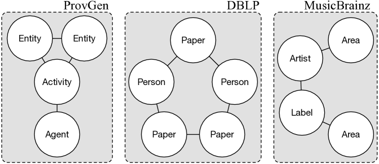
Figure 6. Examples of $q$ for MusicBrainz, DBLP & ProvGen

Table 1 presents information about each of our chosen datasets, including their size and how heterogeneous they are ($|L_{V}|$). We use the DBLP, and LUBM datasets, which are well known. MusicBrainz is a freely available database of curated music metadata, with vertex labels such as Artist, Country, Album and Label. ProvGen(Firth and Missier, 2014) is a synthetic generator for PROV metadata (Moreau et al., 2012), which records detailed provenance for digital artifacts.

5.1.2. Query workloads

For each dataset we must propose a representative query workload to execute so that we may measure partitioning quality in terms of $ipt$. Remember that a query workload consists of a set of distinct query patterns along with a frequency for each (Sec. 1.3). The LUBM dataset provides a set of query patterns which we make use of. For every other dataset, however, we define a small set of common-sense queries which focus on discovering implicit relationships in the graph, such as potential collaboration between authors or artists . The full details of these query patterns are elided for space, however Fig. 6 presents some examples.

Dataset	$\sim|V|$	$\sim|E|$	$|L_{V}|$	Real	Description
DBLP	1.2M	2.5M	8	Y	Publications & citations
ProvGen	0.5M	0.9M	3	N	Wiki page provenance
MusicBrainz	31M	100M	12	Y	Music records metadata
LUBM-100	2.6M	11M	15	N	University records
LUBM-4000	131M	534M	15	N	University records

Table 1. Graph datasets, incl. size & heterogeneity

Note that whilst the TPSTry++ may be trivially updated to account for change in the frequencies of workload queries (Sec. 2), our evaluation of Loom assumes that said frequencies are fixed and known a priori. Recall that, for online databases, we argue this is a realistic assumption (Sec. 1). However, more complete tests with changing workloads are an important area for future work.

5.2. Comparison of systems

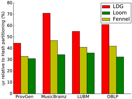
(a) Random order

(b) Breadth-first order

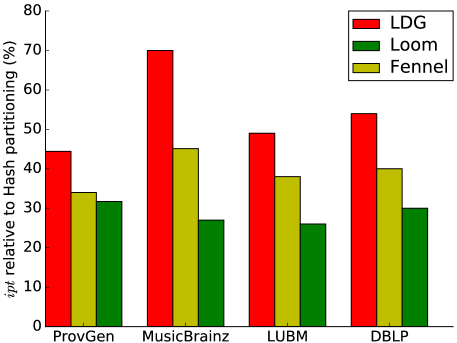
(c) Depth-first order

Figure 7. $ipt$ %, vs. Hash, when executing $Q$ over 8-way partitionings of graph streams in multiple orders.

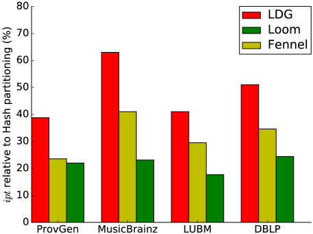
(a) $k=2$

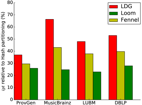
(b) $k=8$

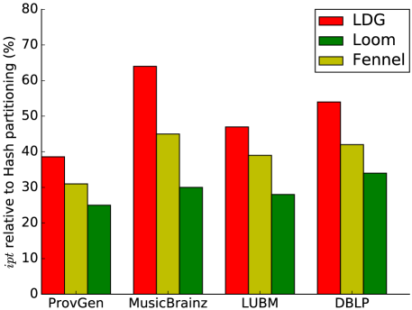
(c) $k=32$

Figure 8. $ipt$ %, vs. Hash, when executing $Q$ over multiple $k$-way partitionings of breadth-first graph streams.

Figures 7 and 8 present the improvement in partitioning quality achieved by Loom and each of the comparable systems we desribe above. Initially, consider the experiment depicted in Fig. 7. We partition ordered streams of each of our first 4 graph datasets into 8-way partitionings, using the approaches described above, then execute each dataset’s query workload over the appropriate partitioning. The absolute number of inter-partition traversals ($ipt$) suffered when querying each dataset varies significantly. Thus, rather than represent these results directly, in Fig. 7 (and 8) we present the results for each approach as relative to the results for Hash; i.e. how many $ipt$ did a partitioning suffer, as a percentage of those suffered by the Hash partitioning of the same dataset.

As expected, the naive hash partitioner performs poorly: it produces partitionings which suffer twice as many inter-partition traversals, on average, when compared to partitionings produced by the next best system (LDG). Whilst the LDG partitioner does achieve around a $55\%$ reduction in $ipt$ vs our Hash baseline, its produces partitionings of consistently poorer quality than those of Fennel and Loom. Although both LDG and Fennel optimise their partitionings for the balanced min. edge-cut goal (Sec. 1), Fennel is the more effective heuristic, cutting around $25\%$ fewer edges than LDG for small numbers of partitions (including $k=8$) (Tsourakakis et al., 2014). Intuitively, the likelihood of any edge being cut is a coarse proxy for the likelihood of a query $q\in Q$ traversing a cut edge. This explains the disparity in $ipt$ scores between the two systems.

Of more interest is comparing the quality of partitionings produced by Fennel and Loom. Fig. 7 clearly demonstrates that Loom offers a significant improvement in partitioning quality over Fennel, given a workload $Q$. Loom’s reduction in $ipt$ relative to Fennel’s is present across all datasets and stream orders, however it is particularly pronounced over ordered streams of more heterogeneous graphs; e.g. MusicBrainz in subfigure 8b, where Loom’s partitioning suffers from $42\%$ fewer $ipt$ than Fennel’s. This makes sense because, as mentioned, pattern matching workloads are more likely to exhibit skew over heterogeneous graphs, where query graphs $G_{q}$ contain a, potentially small, subset of the possible vertex labels. Across all the experiments presented in Fig. 7, the median range of Loom’s $ipt$ reduction relative to Fennel’s is $20-25\%$. Additionally, Fig. 8 demonstrates that this improvement is consistent for different numbers of partitions. As the number of partitions $k$ grows, there is a higher probability that vertices belonging to a motif match are assigned across multiple partitions. This results in an increase of absolute $ipt$ when executing $Q$ over a Loom partitioning. However, increasing $k$ actually increases the probability that any two vertices which share an edge are split between partitions, thus reducing the quality of Hash, LDG and Fennel partitionings as well. As a result, the difference in relative $ipt$ is largely consistent between all 4 systems.

On the other hand, neither Fig. 7, nor Fig. 8, present the runtime costs of producing a partitioning. Table 2 presents how long (in ms) each partitioner takes to partition 10k edges. Whilst all 3 algorithms are capable of partitioning many 10s of thousands of edges per second, we do find that Loom is slower than LDG and Fennel by an average factor of 2-3. This is likely due to the more complex map-lookup and pattern-matching logic performed by Loom, or a nascent implementation. The runtime performance of Loom varies depending on the query workload $Q$ used to generate the TPSTry++ (Sec. 2), therefore the performance figures presented in Table 2 are averaged across many different $Q$. The minimum slowdown factor observed between Loom and Fennel was 1.5, the maximum 7.1. Note that popular non-streaming partitioner Metis (Karypis and Kumar, 1997) is around 13 times slower than Fennel for large graphs (Tsourakakis et al., 2014).

Dataset	LDG (ms)	Fennel (ms)	Loom (ms)	Hash (ms)
DBLP	91	96	235	28
ProvGen	144	146	240	33
MusicBrainz	48	52	129	18
LUBM-100	47	51	147	22
LUBM-4000	45	49	138	16

Table 2. Time to partition 10k edges

We contend that this performance difference is unlikely to be an issue in an online setting for two reasons. Firstly, most production databases do not support more than around 10k transactions per second (TPS) (Lee et al., 2008). Secondly, it is considered exceptional for even applications such as twitter to experience $>$30k-40k TPS . Meanwhile, the lowest partitioning rate exhibited by Loom in Table 2 is equivalent to ~ 42k edges per second, the highest 72k.

Note that Figures 7 and 8 do not present the relative $ipt$ figures for the LUBM-4000 dataset. This is because measuring relative $ipt$ involves reading a partitioned graph into memory, which is beyond the constraints of our present experimental setup. However, we include the LUBM-4000 dataset in Table 2 to demonstrate that, as a streaming system, Loom is capable of partitioning large scale graphs. Also note that none of the figures present partitioning imbalance as this is broadly similar between all approaches and datasets , with LDG varying between $1\%-3\%$, Loom and Fennel between $7\%$ and their maximum imbalance of $10\%$ (Sec. 4).

5.3. Effect of stream order and window size

Fig. 7 indicates that Loom is sensitive to the ordering of its given graph stream. In fact, subfigure 7a shows Loom achieve a smaller reduction in $ipt$ over Fennel and LDG, than in 7b and 7c. Specifically Loom achieves a $42\%$ greater reduction in relative $ipt$ than Fennel given a breadth-first stream of the MusicBrainz graph, but only a $26\%$ when the stream is ordered randomly, despite Fennel and LDG also being sensitive to stream ordering (Stanton and Kliot, 2012; Tsourakakis et al., 2014). This implies that Loom is particularly sensitive to random orderings: edges which are close to one another in the graph may not be close in the graph stream, resulting in Loom detecting fewer motif matching subgraphs in its stream window.

Intuitively, this sensitivity can be ameliorated by increasing the size of Loom’s window, as shown in Fig. 9 As Loom’s window grows, so does the probability that clusters of motif matching subgraphs will occur within it. This allows Loom’s equal opportunism heuristic to make the best possible allocation decisions for the subgraph’s constituent vertices. Indeed, the number of $ipt$ suffered by Loom partitionings improves significantly, by as much as $47\%$, as the window size grows from 100 to 10k. However, increasing the window size past $10$k clearly has little effect on $ipt$ suffered to execute $Q$ if your graph stream is ordered. The exact impact of increasing Loom’s window size depends upon the degree distribution of the graph being partitioned. However, to gain an intuition consider the naive case of a graph with a uniform average vertex degree of 8, along with a TPSTry++ whose largest motif contains 4 edges. In this case, a breadth-first traversal of $8^{4}$ edges from a vertex $a$ (i.e. window size $t\approx 4k$) is highly likely to include all the motif matches which contain $a$. Regardless, Fig. 9 might seem to suggest that Loom should run with the largest window size possible. However, besides the additional computational cost of detecting more motif matches, remember that Loom’s window constitutes a temporary partition (sec. 3). If there exist many edges between other partitions and $P_{temp}$, then this may itself be a source of $ipt$ and poor query performance.

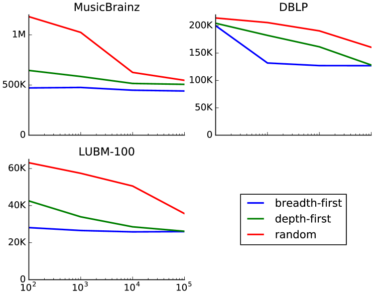
Figure 9. $ipt$ (y-axis) when executing $Q$ over Loom partitionings with multiple window sizes $t$(x-axis)

6. Conclusion

In this paper, we have presented Loom: a practical system for producing $k$-way partitionings of online, dynamic graphs, which are optimised for a given workload of pattern matching queries $Q$. Our experiments indicate that Loom significantly reduces the number of inter-partition traversals ($ipt$) required when executing $Q$ over its partitionings, relative to state of the art (workload agnostic) streaming partitioners.

There are several ways in which we intend to expand our current work on Loom. In particular, as a workload sensitive technique, Loom generates partitionings which are vulnerable to workload change over time. In order to address this we must integrate Loom with an existing, workload sensitive, graph re-partitioner (Firth and Missier, 2017) or consider some form of restreaming approach (Huang and Abadi, 2016).

References

- (1)
- Andreev and Racke (2006) K. Andreev and H. Racke. 2006. Balanced Graph Partitioning. Theory of Computing Systems 39, 6 (2006), 929–939.
- Chevalier and Pellegrini (2008) C. Chevalier and F. Pellegrini. 2008. PT-Scotch: A tool for efficient parallel graph ordering. Parallel Comput. 34, 6-8 (2008), 318–331.
- Choudhury et al. (2015) S. Choudhury, L. Holder, G. Chin, et al. 2015. A Selectivity based approach to Continuous Pattern Detection in Streaming Graphs. Proc. EDBT (2015), 157–168.
- Curino et al. (2010) C. Curino, E. Jones, Y. Zhang, et al. 2010. Schism. Proc. VLDB 3, 1-2 (2010), 48–57.
- Dey et al. (2013) S. Dey, V. Cuevas-Vicenttín, S. Köhler, et al. 2013. On implementing provenance-aware regular path queries with relational query engines. In Proc. EDBT/ICDT Workshops. 214–223.
- Firth and Missier (2014) H. Firth and P. Missier. 2014. ProvGen: Generating Synthetic PROV Graphs with Predictable Structure. In Proc. IPAW. 16–27.
- Firth and Missier (2016) Hugo Firth and Paolo Missier. 2016. Workload-aware Streaming Graph Partitioning.. In Proc. EDBT/ICDT Workshops.
- Firth and Missier (2017) H. Firth and P. Missier. 2017. TAPER: query-aware, partition-enhancement for large, heterogenous graphs. Distributed and Parallel Databases 35, 2 (2017), 85–115.
- Gupta et al. (2014) P. Gupta, V. Satuluri, A. Grewal, et al. 2014. Real-time twitter recommendation. Proc. VLDB 7, 13 (2014), 1379–1380.
- Huang and Abadi (2016) J. Huang and D. Abadi. 2016. LEOPARD : Lightweight Edge-Oriented Partitioning and Replication for Dynamic Graphs. Proc. VLDB 9, 7 (2016), 540–551.
- Jiang et al. (2004) C. Jiang, F. Coenen, and M. Zito. 2004. A Survey of Frequent Subgraph Mining Algorithms. The Knowledge Engineering Review 000 (2004), 1–31.
- Jindal and Dittrich (2012) A. Jindal and J. Dittrich. 2012. Relax and let the database do the partitioning online. In Enabling Real-Time Business Intelligence. 65–80.
- Karypis and Kumar (1997) G. Karypis and V. Kumar. 1997. Multilevel k -way Partitioning Scheme for Irregular Graphs. J. Parallel and Distrib. Comput. 47, 2 (1997), 109–124.
- Kernighan and Lin (1970) B. Kernighan and S. Lin. 1970. An efficient heuristic procedure for partitioning graphs. Bell systems technical journal 49, 2 (1970), 291–307.
- Lee et al. (2008) S. Lee, B. Moon, C. Park, et al. 2008. A case for flash memory ssd in enterprise database applications. In Proc. SIGMOD. 1075.
- Lidl and Niederreiter (1997) R. Lidl and H. Niederreiter. 1997. Finite Fields. Encyclopedia of Mathematics and Its Applications (1997), 1983.
- Margo and Seltzer (2015) D. Margo and M. Seltzer. 2015. A scalable distributed graph partitioner. Proc. VLDB 8, 12 (2015), 1478–1489.
- McKay (1981) B. McKay. 1981. Practical graph isomorphism. (1981), 45–87 pages.
- Mendelzon and Wood (1995) A. Mendelzon and P. Wood. 1995. Finding Regular Simple Paths in Graph Databases. SIAM J. Comput. 24, 6 (1995), 1235–1258.
- Moreau et al. (2012) L. Moreau, P. Missier, K. Belhajjame, et al. 2012. PROV-DM: The PROV Data Model. Technical Report. World Wide Web Consortium.
- Nishimura and Ugander (2013) J. Nishimura and J. Ugander. 2013. Restreaming graph partitioning. In Proc. SIGKDD. New York, New York, USA, 1106–1114.
- Pavlo et al. (2012) A. Pavlo, C. Curino, and S. Zdonik. 2012. Skew-aware automatic database partitioning in shared-nothing, parallel OLTP systems. In Proc. SIGMOD. 61.
- Peng et al. (2016) P. Peng, L. Zou, L. Chen, et al. 2016. Query Workload-based RDF Graph Fragmentation and Allocation. In Proc. EDBT. 377–388.
- Pujol et al. (2010) Josep M Pujol, Vijay Erramilli, Georgos Siganos, Xiaoyuan Yang, Nikos Laoutaris, Parminder Chhabra, and Pablo Rodriguez. 2010. The little engine(s) that could. In Proc. SIGCOMM. 375–386.
- Quamar et al. (2013) A. Quamar, K. Kumar, and A. Deshpande. 2013. SWORD. In Proc. EDBT. 430.
- Ribeiro and Silva (2014) P. Ribeiro and F. Silva. 2014. G-Tries: a data structure for storing and finding subgraphs. Data Mining and Knowledge Discovery 28, 2 (2014), 337–377.
- Shang and Yu (2013) Z. Shang and J. Yu. 2013. Catch the Wind: Graph workload balancing on cloud. Proc. International Conference on Data Engineering (ICDE) (2013), 553–564.
- Song et al. (2014) C. Song, T. Ge, C. Chen, and J. Wang. 2014. Event pattern matching over graph streams. Proc. VLDB 8, 4 (2014), 413–424.
- Stanton and Kliot (2012) I. Stanton and G. Kliot. 2012. Streaming graph partitioning for large distributed graphs. In Proc. SIGKDD. 1222–1230.
- Tsourakakis et al. (2014) C. Tsourakakis, C. Gkantsidis, B. Radunovic, et al. 2014. FENNEL. In Proc. ACM International conference on Web search and data mining (WSDM). 333–342.
- Xu et al. (2014) N. Xu, L. Chen, and B. Cui. 2014. LogGP. Proc. VLDB 7, 14 (2014), 1917–1928.