Improving Palliative Care with Deep Learning

Abstract

Improving the quality of end-of-life care for hospitalized patients is a priority for healthcare organizations. Studies have shown that physicians tend to over-estimate prognoses, which in combination with treatment inertia results in a mismatch between patients wishes and actual care at the end of life . We describe a method to address this problem using Deep Learning and Electronic Health Record (EHR) data, which is currently being piloted, with Institutional Review Board approval, at an academic medical center. The EHR data of admitted patients are automatically evaluated by an algorithm, which brings patients who are likely to benefit from palliative care services to the attention of the Palliative Care team. The algorithm is a Deep Neural Network trained on the EHR data from previous years, to predict all-cause 3-12 month mortality of patients as a proxy for patients that could benefit from palliative care. Our predictions enable the Palliative Care team to take a proactive approach in reaching out to such patients, rather than relying on referrals from treating physicians, or conduct time consuming chart reviews of all patients. We also present a novel interpretation technique which we use to provide explanations of the model’s predictions.

I Introduction

Studies have shown that approximately 80% of Americans would like to spend their final days at home if possible, but only 20% do [1]. In fact, up to 60% of deaths happen in an acute care hospital, with patients receiving aggressive care in their final days. Access to palliative care services in the United States has been on the rise over the past decade. In 2008, 53% of all hospitals with fifty or more beds reported having palliative care teams, rising to 67% in 2015[2]. However, despite increasing access, data from the National Palliative Care Registry estimates that less than half of the 7-8% of all hospital admissions that need palliative care actually receive it[3]. Though a significant reason for this gap comes from the palliative care workforce shortage [4], and incentives for health systems to employ them, technology can still play a crucial role by efficiently identifying patients who may benefit most from palliative care, but might otherwise be overlooked under current care models.

We focus on two aspects of this problem. First, physicians may not refer patients likely to benefit from palliative care for multiple reasons such as overoptimism, time pressures, or treatment inertia [5]. This may lead to patients failing to have their wishes carried out at end of life[6] and overuse of aggressive care. Second, a shortage of palliative care professionals makes proactive identification of candidate patients via manual chart review an expensive and time-consuming process.

The criteria for deciding which patients benefit from palliative care can be hard to state explicitly. Our approach uses deep learning to screen patients admitted to the hospital to identify those who are most likely to have palliative care needs. The algorithm addresses a proxy problem - to predict the mortality of a given patient within the next 12 months - and use that prediction for making recommendations for palliative care referral. This frees the palliative care team from manual chart review of every admission and helps counter the potential biases of treating physicians by providing an objective recommendation based on the patient’s EHR. Currently existing tools to identify such patients have limitations, and they are discussed in the next section.

II Related work

Accurate prognostic information is valuable to patients, caregivers, and clinicians [7] [8]. Several studies have shown that clinicians are generally over optimistic in their estimates of the prognoses of terminally ill patients[9] [5] [10] [11]. It has also been shown that no subset of clinicians are better at late stage prognostication than than others [12] [13] . However, clinician judgment remains the most common method of predicting survival in practice [12]. Several solutions exist that attempt to make patient prognosis more objective and automated. Many of these solutions are models that produce a score based on the patient’s clinical and biological parameters, and can be mapped to an expected survival rate.

Prognostic tools in Palliative Care

The Palliative Performance Scale [14] was developed as a modification of the Karnofsky Performance Status Scale (KPS) [15] to the Palliative care setting, and is calculated based on observable factors such as: degree of ambulation, ability to do activities, ability to do self-care, food and fluid intake, and state of consciousness. The Palliative Prognostic Score (PPS) was constructed for the Palliative Care setting as well, focusing on terminally ill cancer patients [16]. The PPS is calculated with multiple regression analysis based on the following variables: Clinical Prediction of Survival (CPS), Karnofsky Performance Status (KPS), anorexia, dyspnea, total white blood count (WBC) and lymphocyte percentage. The Palliative Prognostic Index (PPI), developed around the same time as PPS, also calculates a multiple regression analysis based score using Performance Status, oral intake, edema, dyspnea at rest, and delirium. These scores are difficult to implement at scale since they involve face-to-face clinical assessment and involve prediction of survival by the clinician. Furthermore, these scores were designed to be used within the palliative care setting, where the patient is already in an advanced stage of the disease — as opposed to identifying them earlier.

Prognostic tools in the Intensive Care Unit

There also are prognosis scoring models that are commonly used in the Intensive Care Unit. The APACHE-II (Acute Physiology, Age, Chronic Health Evaluation) Score predicts hospital mortality risk for critically ill hospitalized adults in the ICU [17]. This model has been more recently refined with the APACHE-III Score, which uses factors such as major medical and surgical disease categories, acute physiologic abnormalities, age, preexisting functional limitations, major comorbidities, and treatment location immediately prior to ICU admission[18]. Another commonly used scoring system in the ICU is the Simplified Acute Physiological Score, or SAPS II [19], which is calculated based on the patient’s physiological and underlying disease variables. While these score are useful for the treatment team when the patient is already in the ICU, they have limited use in terms of identifying patients who are at risk of longer term mortality, while they are still capable of having a meaningful discussion of their goals and values, so that they can be set on an alternative path of care.

Prognostic tools for Early Identification

There have been a number of studies and tools developed that aim to identify terminally ill patients early enough for an end-of-life plan and care to be meaningful.

CriSTAL (Criteria for Screening and Triaging to Appropriate aLternative care) was developed to identify elderly patients nearing end of life, and quantifies the risk of death in the hospital or soon after discharge [20]. CriSTAL provides a check list using eighteen predictors with the goal of identifying the dying patient.

CARING is a tool that was developed to identify patients who could benefit from palliative care[21]. The goal was to use six simple criteria in order to identify patients who were at risk of death within 1 year. PREDICT [22] is a screening tool also based on six prognostic indicators, which were refined from CARING. The model was derived from 976 patients.

The Intermountain Mortality Risk score is an all-causes mortality prediction based on common laboratory tests [23]. The model provides score for 30-day, 1-year and 5-year mortality risk. It was trained on a population of 71,921 and tested on 47,458.

Cowen, M et al [24] proposed using a twenty-four factor based prediction rule at the time of hospital admission to identify patients with high risk of 30-day mortality, and to organize care activities using this prediction as a context. One of the their motivation was to have a rule from a single set of factors, and not be disease specific. The model was derived from 56,003 patients.

Meffert, C et al [25] proposed a scoring method based on logistic regression on six factors to identify hospitalized patients in need of palliative care. In this prospective study, they asked the treating physician at the time of discharge whether the patient had palliative care needs. The trained model was then used to identify such patients at the time of admission. The model was derived from 39,849 patients.

Ramachandran, K et al [26] developed a 30-day mortality prediction tool for hospitalized cancer patients. Their model used eight variables that were based on information from the first 24 hours of admission, and laboratory results and vitals. A logistic regression model was developed from these eight variables and used as a scoring function. The model was derived from 3,062 patients.

Amarasingham, R et al [27] built a tool to screen patients who were admitted with heart failure, and identify those who are at risk of 30-day readmission or death. Their regression model uses a combination of Tabak Morality Score [28], markers of social, behavioral, and utilization activity that could be obtained electronically, ICD-9 CM codes specific to depression and anxiety, billing and administrative data. Though this study was not specifically focused on palliative care, the methodology of using EHR system data is relevant to our work. The model was derived from 1,372 patients.

Makar, M et al [29] used only Medicare claims data on older population ($\geq$ 65 years) to predict mortality in six months. By limiting their model to use only administrative data, they hypothesized an easier deployment scenario thereby making automated prognostic models more prevalent. The model was derived separately on four cohorts (one per disease type) with 20,000 patients per cohort.

Prognosis in the age of Big-Data

The proliferation of EHR systems in healthcare combined with advances in Machine Learning techniques on high dimensional data provides a unique opportunity to make contributions, especially in disease prognosis [30][31]. All the tools described above, and those we reviewed [32] [33] [34] [35] [36], have at least one of the following limitations. They were either derived from small data sets (limited to specific studies or cohorts), or used too few variables (intentionally to make the model portable, or avoid overfitting), or the model was too simple to capture the complexities and subtleties of human health, or was limited to certain sub-populations (based on disease type, age etc.) We address these limitations in our work.

III Methods

We approach the problem of predicting mortality from the point of view of the palliative care team by being largely agnostic to disease type, disease stage, severity of admission (ICU vs non-ICU), age etc. We take a data driven approach and build a deep learning model that considers every patient in the EHR (with a sufficiently long history), without limiting our analysis to any specific sub-population or cohort. In order to make the problem of identifying patients with palliative care needs tractable, we use the following proxy problem statement instead:

Given a patient and a date, predict the mortality of that patient within 12 months from that date, using EHR data of that patient from the prior year.

We treat this as a binary classification problem and build a supervised deep learning model to solve it. Other than building a model that performs well on the above problem, we are also separately interested in the model performance on a sub-problem — the ability to predict mortality of patients who are currently admitted. This is because it is much easier for the palliative care staff to intervene with admitted patients.

Data Source

STRIDE (Stanford Translational Research Integrated Database Environment) [37] is a clinical data warehouse supporting clinical and translational research at Stanford University. The snapshot of STRIDE used in our work comprises the EHR data of approximately 2 million adult and pediatric patients cared for at either the Stanford Hospital or the Lucile Packard Children’s hospital between 1995 and 2014.

Constructing a Dataset for Supervised Learning

Patients who have a recorded date of death are considered positive cases; other patients are considered negative cases. Further, we define the prediction date of a patient to be the point in time that divides their health record timeline into virtual future and past events. We use data from each patient’s virtual past to make predictions about their survival 3-12 months in the future. Note that we must take care when defining the prediction date to not violate common sense constraints (described below) that could invalidate the labels. We only include patients for whom it is possible to find a prediction date that satisfies these constraints.

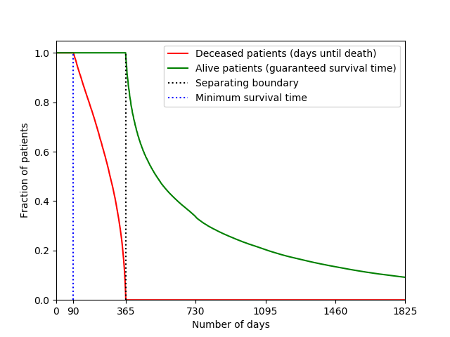
Figure 1: Right-censoring lengths shown as a survival plot.

Positive Cases

The constraints for positive cases were decided based on the rationale that palliative care is most beneficial if the referral occurs 3-12 months prior to death. Predicting mortality within 3 months is considered too late due to the preparatory time required to start palliative care in general. On the other hand, a lead time longer than 12 months is problematic because making accurate predictions over such a long time horizon is difficult, and more importantly, palliative care interventions are a limited resource that are best focused on more immediate needs. The prediction date for positive cases must meet all the following constraints:

• The prediction date must be a recorded date of encounter.

• The prediction date must be at least 3 months prior to date of death (otherwise death is too near).

• The prediction date can be at most 12 months prior to date of death (otherwise death is too far).

• The prediction date must be at least 12 months after the date of first encounter (otherwise the patient lacks sufficient history on which to base a prediction).

• In-patient admissions are preferred over other admission types for the prediction date, as long as they meet the previous constraints (since it is easier to start the palliative care conversation with them).

• The prediction date must be the earliest among the possible candidate dates subject to previous constraints.

Negative Cases

For negative cases (patients without a date of death), we require that the patient was alive for at least 12 months from the prediction date. We choose the prediction date such that it satisfies all the following constraints:

• The prediction date must be a recorded date of encounter.

• The prediction date must be at least 12 months prior to date of last encounter (to avoid ambiguity of death after date of EHR snapshot).

• The prediction date must be at least 12 months after the date of first encounter (otherwise insufficient history).

• In-patient admissions are preferred over other encounter types for the prediction date, as long as they meet the previous constraints (to serve as controls for the admitted positive cases).

• The prediction date must be the latest among the possible candidate dates subject to previous constraints.

Admitted patients

Those patients whose prediction date corresponds to an in-patient admission are considered admitted patients. Remaining patients are considered non-admitted (note that non-admitted patients could still have other recorded admissions in their history). Further, for admitted patients, their prediction date it is re-adjusted by incrementing it to be the second day of admission. The rationale for doing this is that patient records are generally updated with the latest data (preliminary tests, diagnostics etc.) within 24 hours of admission, and the second day is better suited for making a more informed prediction. Note that the admitted patients are a subset of the included patients (and NOT a separate set).

All the data after the prediction date is censored in both the positive and negative cases. The KM-plot of censor lengths is shown in Fig 1, highlighting the separation between the two classes at 365 days.

Data Description

	Alive	Deceased	Total
In EHR	1,880,096	131,009	201,1105
Selected	205,571	15,713	221,284
Admitted	9,648	1,131	10,779

TABLE I: Breakdown of patient counts.

The inclusion criteria selected a total of 221,284 patients. Table  I shows the breakdown of these patients based on inclusion and admission.

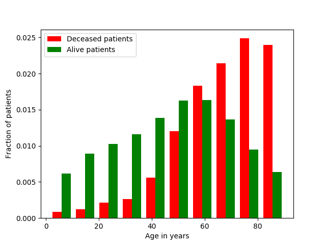
Figure 2: Age of patients at prediction time.

We observe that, unsurprisingly, the distribution of age at prediction time is not equal between the classes, and that the positive class (of deceased patients) is skewed towards older age (Fig  2).

	Training	Validation	Testing
Alive	164,424	20,619	20,528	205,571
Deceased	12,587	1,520	1,606	15,713
	177,011	22,139	22,134	221,284

TABLE II: Data split for modeling.

The included patients are randomly split in approximate ratio 8:1:1 into training, validation and test sets, as shown in Table II.

The prevalence of death among the included patients is approximately 7%. Approximately 5% were admitted patients (i.e., prediction date was the second day of an admission). Among the admitted patients, the prevalence of death is about 11%.

Feature Extraction

For each patient, we consider the 12 months leading up to their prediction date as their observation window. Within the observation window of each patient, we use ICD9 (International Classification of Diseases 9th rev) diagnostic and billing codes, CPT (Current Procedural Terminology) procedure codes, RxNorm prescription codes, and encounters found in that period to create features.

	Start date	End date	Duration
observation window	PD - 365	PD	365
observation slice 1	PD - 30	PD	30
observation slice 2	PD - 90	PD - 30	60
observation slice 3	PD - 180	PD - 90	90
observation slice 4	PD - 365	PD - 180	185

TABLE III: Observation window and slices

We create features as follows. In order to capture the longitudinal nature of the data, we split the observation window of each patient into four observation slices, specified relative to the prediction date (PD) as shown in Table III

Thus, observation slice 1 is the most recent, and 4 is the oldest. The slice widths are intentionally uneven in order to give more emphasis to recent data. Within each observation slice, we count the the number of occurrences of each code in each code category (prescription, billing, etc.) per patient. The count of every such code within the slice is considered a separate feature.

We also include the patient demographics (age, gender, race and ethnicity), and the following per-patient summary statistics in the observation window for each code category:

• Count of unique codes in the category.

• Count of total number of codes in the category.

• Maximum number of codes assigned in any day.

• Minimum number of codes (non-zero) assigned in any day.

• Range of number of codes assigned in a day.

• Mean of number of codes assigned in a day.

• Variance in number of codes assigned in a day.

All these features (i.e, code counts in each of the four observation slices, per category summary statistics over the observation window, and demographics) were concatenated to form the candidate feature set. From this set, we pruned away those features which occur in 100 or fewer patients. This resulted in the final set of 13,654 features. Of the 13,654 features, each patient on average has 74 non-zero values (with a standard deviation of 62), and up to a maximum of 892 values. The overall feature matrix is approximately 99.5% sparse.

Algorithm and Training

Our model is a Deep Neural Network (DNN) [38] comprising an input layer (of 13,654 dimensions), 18 hidden layers (each 512 dimensions) and a scalar output layer. We employ the logistic loss function at the output layer and use the Scaled Exponential Linear Unit (SeLU) activation function [39] at each layer. The model is optimized using the Adam optimizer [40], with a mini-batch size of 128 examples. Intermediate model snapshots were taken every 250 mini-batch iterations, and the snapshot that performed best on the validation test was selected as the final model. Explicit regularization was not found necessary. The network configuration was reached by extensive hyperparameter search over various network depths (ranging from 2 to 32) and activation functions ($tanh$, $ReLU$ and $SeLU$).

The software was implemented using the Python programming language (version 2.7), PyTorch framework [41], and the scikit-learn library (version 0.17.1) [42]. The training was performed on an NVIDIA TitanX (12GB RAM) with CUDA version 8.0.

Evaluation

Since the data is imbalanced (with 7% prevalence), accuracy can be a poor evaluation metric [43]. The ROC curve can also be sometimes misleading on imbalanced problems[44] [45]. Therefore, we use the Average Precision (AP) score, also known as Area Under Precision-Recall Curve (AUPRC) for model selection [46].

IV Results

Patient MRN	XXXXXXX
Probability score	0.946

Factors	Code	Value	Influence	Description
Top Diagnostic factors	V10.51	4	0.0051	Personal history of malignant neoplasm of bladder
	V10.46	5	0.0019	Personal history of malignant neoplasm of prostate
	518.5	1	0.0012	Pulmonary insufficiency following trauma and surgery
	518.82	1	0.0008	Other pulmonary insufficiency
	88.75	1	0.0006	Diagnostic ultrasound of urinary system
Top Procedural factors	88331	1	0.0017	Pathology consultation during surgery with FS
	75984	1	0.0014	Transcatheter Diagnostic Radiology Procedure
	72158	1	0.0013	MRI and CT Scans of the Spine
	Code_Type_Count	76	0.0011	Summary statistic (count of all ICD/CPT codes)
	76005	1	0.0007	Fluroscopic guidance and localization of needle or catheter tip for spine
Top Medication factors
Top Encounter factors	Hx Scan	21	0.0012	Number of scan encounters of all types
	Inpatient	60	0.0004	Number of days patient was admitted
	Var_Codes_per_Day	8	0.0002	Summary statistic (variance in number of codes assigned per day)
	Code_Day_Count	88	0.0001	Number of days any encounter code was assigned
Top Demographic factors	Age	81	0.0010	Age of patient in years at prediction time

TABLE IV: Prediction explanation generated on a random positive patient with high probability score. Only factors that contributed to a drop in probability score are reported.

Patient MRN	YYYYYYY
Probability score	0.909

Factors	Code	Value	Influence	Description
Top Diagnostic factors	197.7	16	0.1299	Malignant neoplasm of liver, secondary
	154.1	3	0.1254	Malignant neoplasm of rectum
	287.5	1	0.0194	Thrombocytopenia, unspecified
	780.6	1	0.0171	Fever and other physiologic disturbances of temperature regulation
	733.90	1	0.0113	Other and unspecified disorders of bone and cartilage
Top Procedural factors	73560	1	0.0502	Diagnostic Radiology (Diagnostic Imaging) Procedures of the Lower Extremities
	Code_Type_Count	20	0.0491	Summary statistic (Number of unique ICD-9/CPT codes)
	74160	1	0.0381	Diagnostic Radiology (Diagnostic Imaging) Procedures of the Abdomen
	Max_Codes_per_Day	6	0.0234	Summary statistic (Maximum number of codes in any day)
	Range_Codes_per_Day	6	0.0233	Summary statistic (Range of codes across days)
Top Medication factors	283838	1	0.0619	Darbepoetin Alfa
	28889	1	0.0247	Loratadine
	Range_Codes_per_Day	5	0.0023	Summary statistic (Ranges of codes across days)
	Max_Codes_per_Day	5	0.0023	Summary statistic (Maximum number of codes in any day)
	Code_Type_Count	6	0.0015	Summary statistic (Number of unique medication codes)
Top Encounter factors	Hx Scan	19	0.2239	Number of scan encounters of all types
	Code_Day_Count	97	0.0284	Number of days any encounter code was assigned
	Outpatient	22	0.0228	Number of Outpatient encounters
	Var_Codes_per_Day	1	0.0074	Summary statistic (variance in number of codes assigned per day)
Top Demographic factors

TABLE V: Prediction explanation generated on a random false positive patient with high probability score. Only factors that contributed to a drop in probability score are reported.

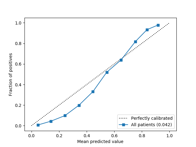
Figure 3: Reliability curve (calibration plot) of the model output probabilities on the test set data.

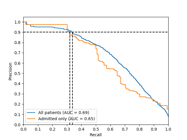
Figure 4: Interpolated Precision-Recall curve. The horizontal dotted line represents precision level of 0.9. The vertical dotted lines indicate the recall at which the curves achieve 0.9 precision.

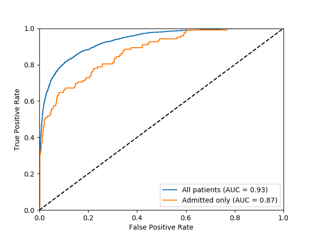
Figure 5: Receiver Operating Characteristic (ROC) of the model performance on the test set.

In this section we report technical evaluation results obtained on the test set using the model selected based on the best AP score on the validation set.

We observe that the model is reasonably calibrated (Fig 3) with a Brier score of 0.042. In the high threshold regime, which is of interest to us, the model is a little conservative (under-confident) in its probability estimates, which should not hurt.

The interpolated Precision-Recall curve is shown in Fig 4. The model achieves an AP score of 0.69 (0.65 on admitted patients). Early recall is desirable, and therefore Recall at precision 0.9 is a metric of interest. The model achieves recall of 0.34 at 0.9 precision (0.32 on admitted patients). The Receiver Operating Characteristic curve is shown in Fig 5. The model achieves an AUROC of 0.93 (0.87 for admitted patients). Both the ROC and Precision-Recall plots suggest that the model demonstrates strong early recall behavior.

Qualitative Analysis

It is worth recalling that predicting mortality was a proxy problem for identifying patients who could benefit from palliative care. In order to evaluate our performance on the original problem, we inspected false positives with high output probability. Although such patients did not die within 12 months from their prediction dates, we noted that they were often diagnosed with terminal illness and/or are high utilizers of healthcare services. This can be seen in the positive and false positive examples shown in Section V.

Upon conducting a chart review of 50 randomly chosen patients in the top 0.9 precision bracket of the test set, the palliative care team found all were appropriate for a referral on their prediction date, even if they survived more than a year. This suggests that mortality prediction was a reasonable (and tractable) choice of a proxy problem to solve.

V Explaining Predictions

Supervised machine learning techniques, and in particular Deep Learning techniques, have recently demonstrated tremendous success in predictive ability. However, better performance often requires larger, more complex models and thus sacrifice interpretability. It is worth drawing a distinction between interpreting a model, versus interpreting its decision [47] [48]. While interpreting complex models (e.g very deep neural networks) may sometimes be infeasible, it is often the case that users only want an explanation for the prediction made by the model for a given example. It is important to establish the trust of the practitioner in the model’s decisions for them to feel comfortable taking actions based on it. Providing explanations along with decisions help establish that trust.

We make the following observations to motivate our explanation technique.

• We can view the EHR data as a strictly growing log of events, and that new data is only added (nothing is modified or removed in general). This results in all our features being positive valued (as counts, means and variance of counts, etc).

• We are most interested in explaining why a model assigns high probability to a patient. We are less interested in getting an explanation for why a healthy person was given a low probability (the reasons are also much less clear: the patient did not have brain cancer, did not have pneumonia, and so on).

• Directly perturbing feature vectors (e.g sensitivity analysis or for techniques described in [47]) does not work well in our case . For example, perturbing the feature representing the ICD count for brain cancer from zero to non zero can increase the probability of death significantly, implying that it is an important factor in general. However, that is not a very useful observation for a specific patient who does not have brain cancer.

These observations motivate the following technique. For each ICD-9, CPT, RXNORM and Encounter code, we ablate all occurrences of that code from the patient’s EHR, create a new feature vector, and measure the drop in probability compared to the original probability. This corresponds to asking: all else being equal, how would the probability change if this patient was not diagnosed with XYZ, prescribed drug ABC, etc? This drop in probability is considered the influence the code has on the model’s decision for that patient. Demographic features are handled as follows. We zero out the age and swap the gender to the opposite sex, and measure the respective drops in probability. Finally we sort the codes in descending order by influence, and pick the top 5 in each code category. A random example of such a positive and false positive case are shown in Table IV and V.

VI Conclusion

We demonstrate that routinely collected EHR data can be used to create a system that prioritizes patients for follow up for palliative care . In our preliminary analysis we find that it is possible to create a model for all-cause mortality prediction and use that outcome as a proxy for the need of a palliative care consultation. The resulting model is currently being piloted for daily, proactive outreach to newly admitted patients. We will collect objective outcome data (such as rates of palliative care consults, and rates of goals of care documentation) resulting from the use of our model . We also demonstrate a novel method of generating explanations from complex deep learning models that helps build confidence of practitioners to act on the recommendations of the system.

References

- [1] Where do americans die? [Online]. Available: https://palliative.stanford.edu/home-hospice-home-care-of-the-dying-patient/where-do-americans-die/
- [2] T. Dumanovsky, R. Augustin, M. Rogers, K. Lettang, D. E. Meier, and R. Sean Morrison, “Special Report The Growth of Palliative Care in U.S. Hospitals: A Status Report.”
- [3] (2015) ”palliative care, report card”. [Online]. Available: https://web.archive.org/web/20170316014732/https://reportcard.capc.org/#key-findings
- [4] J. Spetz, N. Dudley, L. Trupin, M. Rogers, D. E. Meier, and T. Dumanovsky, “Few Hospital Palliative Care Programs Meet National Staffing Recommendations.” Health affairs (Project Hope), vol. 35, no. 9, pp. 1690–7, 9 2016.
- [5] N. Christakis and E. Lamont, “Extent and determinants of error in doctors’ prognoses in terminally ill patients: prospective cohort study,” BMJ, 2000.
- [6] (2014) ”most physicians would forgo aggressive treatment for themselves at the end of life, study finds”. [Online]. Available: https://med.stanford.edu/news/all-news/2014/05/most-physicians-would-forgo-aggressive-treatment-for-themselves-.html
- [7] J. S. Kutner, J. F. Steiner, K. K. Corbett, D. W. Jahnigen, and P. L. Barton, “Information needs in terminal illness.”
- [8] K. E. Steinhauser, N. A. Christakis, E. C. Clipp, M. Mcneilly, S. Grambow, J. Parker, and J. A. Tulsky, “Preparing for the End of Life: Preferences of Patients, Families, Physicians, and Other Care Providers,” Journal of Pain and Symptom Management J Pain Symptom Manage, vol. 2222, no. 727, 2001.
- [9] D. Selby, A. Chakraborty, T. Lilien, E. Stacey, L. Zhang, and J. Myers, “Clinician Accuracy When Estimating Survival Duration: The Role of the Patient’s Performance Status and Time-Based Prognostic Categories,” Journal of Pain and Symptom Management, vol. 42, no. 4, pp. 578–588, 10 2011.
- [10] A. Viganò, M. Dorgan, E. Bruera, and M. E. Suarez-Almazor, “The Relative Accuracy of the Clinical Estimation of the Duration of Life for Patients with End of Life Cancer.”
- [11] P. Glare, C. Sinclair, M. Downing, P. Stone, M. Maltoni, and A. Vigano, “Predicting survival in patients with advanced disease,” vol. 4, no. 2, 2008.
- [12] N. White, F. Reid, A. Harris, P. Harries, P. Stone, and N. Pulenzas, “A Systematic Review of Predictions of Survival in Palliative Care: How Accurate Are Clinicians and Who Are the Experts?” PLOS ONE, vol. 11, no. 8, p. e0161407, 8 2016.
- [13] D. O. Macmillan, “Accuracy of prediction of survival by different professional groups in a hospice,” Palliative Medicine, vol. 12, pp. 117–118, 1998.
- [14] F. Lau, G. M. Downing, M. Lesperance, J. Shaw, and C. Kuziemsky, “Use of Palliative Performance Scale in End-of-Life Prognostication,” JOURNAL OF PALLIATIVE MEDICINE, vol. 9, no. 5, 2006.
- [15] D. A. Karnofsky, W. H. Abelmann, L. F. Craver, and J. H. Burchenal, “The use of the nitrogen mustards in the palliative treatment of carcinoma.With particular reference to bronchogenic carcinoma,” Cancer, vol. 1, no. 4, pp. 634–656, 11 1948.
- [16] M. Pirovano, M. Maltoni, O. Nanni, M. Marinari, M. Indelli, G. Zaninetta, V. Petrella, S. Barni, E. Zecca, E. Scarpi, R. Labianca, D. Amadori, and G. Luporini, “A New Palliative Prognostic Score: A First Step for the Staging of Terminally Ill Cancer Patients for the Italian Multicenter and Study Group on Palliative Care,” Journal of Pain and Symptom Management Pirovano et al, vol. 17, no. 4, 1999.
- [17] W. A. Knaus, E. A. Draper, D. P. Wagner, and J. E. Zimmerman, “APACHE II: a severity of disease classification system.” Critical care medicine, vol. 13, no. 10, pp. 818–29, 10 1985.
- [18] W. A. Knaus, D. P. Wagner, E. A. Draper, J. E. Zimmerman, M. Bergner, P. G. Bastos, C. A. Sirio, D. J. Murphy, T. Lotring, A. Damiano, and F. E. Harrell, “The APACHE III Prognostic System,” Chest, vol. 100, no. 6, pp. 1619–1636, 12 1991.
- [19] J.-R. Le Gall, S. Lemeshow, and F. Saulnier, “A New Simplified Acute Physiology Score (SAPS II) Based on a European/North American Multicenter Study,” JAMA: The Journal of the American Medical Association, vol. 270, no. 24, p. 2957, 12 1993.
- [20] M. Cardona-Morrell and K. Hillman, “Development of a tool for defining and identifying the dying patient in hospital: Criteria for Screening and Triaging to Appropriate aLternative care (CriSTAL).” BMJ supportive & palliative care, vol. 5, no. 1, pp. 78–90, 3 2015.
- [21] S. M. Fischer, W. S. Gozansky, A. Sauaia, S.-J. Min, J. S. Kutner, and A. Kramer, “A Practical Tool to Identify Patients Who May Benefit from a Palliative Approach: The CARING Criteria.”
- [22] P. Richardson, J. Greenslade, S. Shanmugathasan, K. Doucet, N. Widdicombe, K. Chu, and A. Brown, “PREDICT: a diagnostic accuracy study of a tool for predicting mortality within one year: Who should have an advance healthcare directive?” Palliative Medicine, vol. 29, no. 1, pp. 31–37, 1 2015.
- [23] B. D. Horne, H. T. May, J. B. Muhlestein, B. S. Ronnow, D. L. Lappé, D. G. Renlund, A. G. Kfoury, J. F. Carlquist, P. W. Fisher, R. R. Pearson, T. L. Bair, and J. L. Anderson, “Exceptional Mortality Prediction by Risk Scores from Common Laboratory Tests,” AJM, vol. 122, pp. 550–558, 2009.
- [24] M. E. Cowen, R. L. Strawderman, J. L. Czerwinski, M. J. Smith, L. K. Halasyamani, and M. E. Cowen, “Mortality predictions on admission as a context for organizing care activities,” Journal of Hospital Medicine, vol. 8, no. 5, pp. 229–235, 5 2013.
- [25] C. Meffert, G. Rücker, I. Hatami, and G. Becker, “Identification of hospital patients in need of palliative care-a predictive score,” 2016.
- [26] K. J. Ramchandran, J. W. Shega, J. Von Roenn, M. Schumacher, E. Szmuilowicz, A. Rademaker, B. B. Weitner, P. D. Loftus, I. M. Chu, and S. Weitzman, “A predictive model to identify hospitalized cancer patients at risk for 30-day mortality based on admission criteria via the electronic medical record,” Cancer, vol. 119, no. 11, pp. 2074–2080, 6 2013.
- [27] R. Amarasingham, B. J. Moore, Y. P. Tabak, M. H. Drazner, C. A. Clark, S. Zhang, W. G. Reed, T. S. Swanson, Y. Ma, and E. A. Halm, “An Automated Model to Identify Heart Failure Patients at Risk for 30-Day Readmission or Death Using Electronic Medical Record Data.”
- [28] Y. P. Tabak, R. S. Johannes, and J. H. Silber, “Using Automated Clinical Data for Risk Adjustment,” Medical Care, vol. 45, no. 8, pp. 789–805, 8 2007.
- [29] M. Makar, M. Ghassemi, D. Cutler, and Z. Obermeyer, “Short-Term Mortality Prediction for Elderly Patients Using Medicare Claims Data.”
- [30] I. Sim, Z. FH, T. SM, H. SY, Z. N, H. Y, and N. M, “Two Ways of Knowing: Big Data and Evidence-Based Medicine,” Annals of Internal Medicine, vol. 164, no. 8, p. 562, 4 2016.
- [31] Z. Obermeyer and E. J. Emanuel, “Predicting the Future - Big Data, Machine Learning, and Clinical Medicine.” The New England journal of medicine, vol. 375, no. 13, pp. 1216–9, 9 2016.
- [32] S. Rose, “Mortality Risk Score Prediction in an Elderly Population Using Machine Learning,” American Journal of Epidemiology, vol. 177, no. 5, pp. 443–452, 3 2013.
- [33] T. L. Wiemken, S. P. Furmanek, W. A. Mattingly, B. E. Guinn, R. Cavallazzi, R. Fernandez-Botran, L. A. Wolf, C. L. English, and J. A. Ramirez, “Predicting 30-day mortality in hospitalized patients with community-acquired pneumonia using statistical and machine learning approaches.” Journal of Respiratory Infections, vol. 1, no. 3, 5 2017.
- [34] M. Motwani, D. Dey, D. S. Berman, G. Germano, S. Achenbach, M. H. Al-Mallah, D. Andreini, M. J. Budoff, F. Cademartiri, T. Q. Callister, H.-J. Chang, K. Chinnaiyan, B. J. W. Chow, R. C. Cury, A. Delago, M. Gomez, H. Gransar, M. Hadamitzky, A. Dunning, J. K. Min, and P. J. Slomka, “Machine learning for prediction of all-cause mortality in patients with suspected coronary artery disease: a 5-year multicentre prospective registry analysis,” Yong-Jin Kim Jonathon Leipsic, vol. 18, no. 23.
- [35] G. F. Cooper, C. F. Aliferis, R. Ambrosino, J. Aronis, and B. G. Buchanon, “An Evaluation of Machine-Learning Methods for Predicting Pneumonia Mortality.”
- [36] J. Vomlel, H. Kružík, P. Tůma, J. Přeček, and M. Hutyra, “Machine Learning Methods for Mortality Prediction in Patients with ST Elevation Myocardial Infarction *.”
- [37] H. J. Lowe, T. A. Ferris, P. M. Hernandez Nd, and S. C. Weber, “STRIDE – An Integrated Standards-Based Translational Research Informatics Platform.”
- [38] Y. LeCun, Y. Bengio, and G. Hinton, “Deep Learning,” Nature, vol. 521, pp. 436–444, 2015.
- [39] G. Klambauer, T. Unterthiner, A. Mayr, and S. Hochreiter, “Self-Normalizing Neural Networks,” 6 2017.
- [40] D. P. Kingma and J. Ba, “Adam: A Method for Stochastic Optimization,” 12 2014.
- [41] Pytorch. [Online]. Available: https://pytorch.org
- [42] F. Pedregosa, G. Varoquaux, A. Gramfort, V. Michel, B. Thirion, O. Grisel, M. Blondel, P. Prettenhofer, R. Weiss, V. Dubourg, J. Vanderplas, A. Passos, D. Cournapeau, M. Brucher, M. Perrot, and E. Duchesnay, “Scikit-learn: Machine learning in Python,” Journal of Machine Learning Research, vol. 12, pp. 2825–2830, 2011.
- [43] Haibo He and E. Garcia, “Learning from Imbalanced Data,” IEEE Transactions on Knowledge and Data Engineering, vol. 21, no. 9, pp. 1263–1284, 9 2009.
- [44] J. Davis and M. Goadrich, “The Relationship Between Precision-Recall and ROC Curves.”
- [45] K. Boyd, V. Santos Costa, J. Davis, and C. D. Page, “Unachievable Region in Precision-Recall Space and Its Effect on Empirical Evaluation.”
- [46] Y. Yuan, W. Su, and M. Zhu, “Threshold-free measures for assessing the performance of medical screening tests.” Frontiers in public health, vol. 3, p. 57, 2015.
- [47] M. T. Ribeiro, S. Singh, and C. Guestrin, “" Why Should I Trust You? " Explaining the Predictions of Any Classifier.”
- [48] Z. C. Lipton, “The Mythos of Model Interpretability.”