Towards a non-perturbative calculation of Weak Hamiltonian Wilson coefficients

Abstract

We propose a method to compute the Wilson coefficients of the weak effective Hamiltonian to all orders in the strong coupling constant using Lattice QCD simulations. We perform our calculations adopting an unphysically light weak boson mass of around $2~{}\mathrm{GeV}$. We demonstrate that systematic errors for the Wilson coefficients $C_{1}$ and $C_{2}$, related to the current-current four-quark operators, can be controlled and present a path towards precise determinations in subsequent works.

I Introduction

Weak decays of hadrons, and in particular of mesons, play an important role in our understanding of the fundamental forces and having precise theoretical predictions to compare against the experimental results can either strenghten the solidity of the Standard Model or lead to discoveries of new physics Buras (2016).

The large scale separation between the mesons, strongly bounded particles with masses of order $\Lambda_{\mathrm{QCD}}$, and the weak mediators with masses around 100 GeV, is used to simplify theoretical predictions of these processes in the framework of effective field theories. By integrating out the heavier degrees of freedom, specifically the weak bosons and heavy quarks, from the Standard Model, it is possible to define a new effective Hamiltonian with new operators and new coupling constants usually called the Wilson coefficients.

The coefficients capture the effect of the weak bosons and heavy quarks that are absent from the effective field theory (EFT), making them well-suited for a perturbative calculation. Instead, matrix elements of the operators involving mesonic external states require a non-perturbative calculation. In the last decade, thanks to algorithmic and computational advances, the Lattice QCD community has been able to cover a wide range of processes involving two mesons (see e.g. LABEL:Aoki:2016frl) and also to complete the first two-body final state decays of $K\to\pi\pi$ Bai et al. (2015); Blum et al. (2012a, b, 2015).

On the other hand perturbative calculations of the Wilson coefficients have been successfully carried out up to NLO (for a comprehensive review see LABEL:Buchalla:1995vs) and in some cases up to NNLO Gorbahn and Haisch (2005). In this work we explore the possibility of a non-perturbative method to compute the Wilson coefficients to address the perturbative uncertainty of the analytic calculations. The perturbative truncation error is traded with the statistical and systematic errors usually present in lattice calculations and the purpose of this paper is to define a methodology to obtain a precise determination of the Wilson coefficients where all uncertainties have been addressed.

The problem of defining the weak effective Hamiltonian non-perturbatively has already had some initial considerations by the authors of LABEL:Dawson:1997ic: by separating two hadronic weak currents and studying their dependence as a function of this distance it is possible to define properly normalized operators, where the effect of the Wilson coefficients has been fitted away by using their perturbative expansion. Our approach differs from the one considered in LABEL:Dawson:1997ic as we plan to directly determine the Wilson coefficients using gauge fixed external quark states, rather than mesons, in momentum space and not in coordinate space.

The rest of the manuscript is organized as follows: in the next section we give an overview of the main features of the EFT and we describe our strategy to measure the Wilson coefficients; in section III we show our results and address the various uncertanties of the calculation; in section IV we report our determination of the Wilson coefficients in the ${\overline{\mathrm{MS}}}$ scheme and discuss the comparison against the known perturbative results, and finally we conclude and present further directions for this project.

II Computational Method

Before introducing the lattice observables and our main strategy, we review the most important features of the EFT.

For concreteness let us restrict to transitions among hadrons. When the weak bosons and the heavy quarks are integrated out, the leading effective field theory that arises is based on operators of dimension 6 with four-quark vertices. This can be easily seen by considering the first term in the expasion of the weak propagator in the limit $m_{\mathrm{W}}\to\infty$. The full expansion however contains other terms that can be related to operators with higher dimensions, in fact the most general form of the effective Hamiltonian is

$$\mathcal{H}_{\mathrm{eff}}=\sum_{i}V^{\mathrm{CKM}}_{i}\frac{G_{\mathrm{F}}}{\sqrt{2}}C_{i}Q_{i}+\sum_{j\,,d_{j}>6}\frac{c_{j}^{(d_{j})}}{m_{\mathrm{W}}^{d_{j}-4}}Q_{j}^{(d_{j})}\,.$$ (1)

In eq. (1) $G_{\mathrm{F}}$ represents the dimensionful Fermi constant which is related to the $SU(2)_{L}$ coupling of the Standard Model $g_{2}$, according to $G_{\mathrm{F}}/\sqrt{2}=g_{2}^{2}/(8m_{\mathrm{W}}^{2})$. $V^{\mathrm{CKM}}_{i}$ denotes a generic product of the usual CKM matrix elements that depends on the flavor structure of the process and consequently of the operators. Note that among the heavy particles that are removed from the theory there is also the top quark, whose presence affects the Wilson coefficients Buchalla et al. (1996); Gorbahn and Haisch (2005).

A reliable computation of the Wilson coefficients $C_{i}$ requires a good suppression of the higher dimensional terms, which is obtained by performing the calculation at energy scales sufficiently small compared to $m_{\mathrm{W}}$. Once the operators in the second sum of eq. (1) can be neglected, the Wilson coefficients are obtained by equating the amplitudes computed in the EFT with the the ones computed in the full theory, which in our case differs from the Standard Model as explained below. Previous perturbative calculations Buchalla et al. (1996) were based on amplitudes computed with off-shell external massless quarks and in our calculation we proceed along these lines. As ultraviolet quantities, the Wilson coefficients are expected to be independent from the infrared regulators of the theory and the external states used in the amplitudes; checking this explicitly will be an important task of our work. Similarly we will also test the gauge invariance of our results in the limit where the amplitudes go on-shell, where any depedence on the weak gauge fixing parameter disappears.

The amplitudes of the EFT require additional renormalization conditions, due to the new divergences that appear, leading to the mixing of the renormalized operators among themselves. Hence, it is important to consider a complete basis of operators that closes under renormalization, such that

$$Q_{i}^{\mathrm{R}}(\mu)=[Z(\mu)]_{ij}\ Q_{j}^{\mathrm{bare}}\,.$$ (2)

The basis of operators depends on the details of the process considered. For instance, a $2\to 2$ transition where the four external quarks have different flavors (e.g. $c\to su\bar{d}$) requires only two current-current operators. Instead, e.g., a basis of 7 independent operators is needed in the 3-flavor EFT (i.e. $\mathcal{H}_{\mathrm{eff}}^{\Delta S=1}$) to describe the $K\to\pi\pi$ process in the zero isospin channel, involving also disconnected contributions that are typically more difficult to compute on the lattice. Therefore, in this exploratory study we will focus only on the simpler current-current operators and consequently only on the Wilson coefficients $C_{1}$ and $C_{2}$.

A third remark concerns the running of the Wilson coefficients, as some care is required in computing them at low scales. In fact, if we naively match the two theories at scales $\mu\ll m_{\mathrm{W}}$ we may encounter large logarithms in the form of $\log(m_{\mathrm{W}}^{2}/\mu^{2})$. Therefore, in order to cancel these terms, the matching is performed exactly at $\mu=m_{\mathrm{W}}$, thus defining the so-called initial conditions of the Wilson coefficients, and their values at scales lower than $m_{\mathrm{W}}$ are obtained by solving their corresponding renormalization group equations. This leads to a resummation of all logarithms of the form $\alpha^{n}\big{(}\alpha\log\frac{m_{\mathrm{W}}^{2}}{\mu^{2}}\big{)}^{k}$ for any power $k$ at fixed loop order $n$. The step-scaling matrix involved in the running of the Wilson coefficients is given by the ratio of $Z$ at two different scales and is a well known and studied problem on the lattice (see e.g. Refs. Boyle et al. (2017); Papinutto et al. (2017)). Instead, in our work we focus on the initial conditions of the Wilson coefficients. More precisely, we compute the matching between a theory with 3 light dynamical quarks in the sea, playing the role of our 3-flavor EFT, with the full theory where we also include the $W$ boson exchange. In this study we do not consider the problem of removing a heavy quark from the theory, which is relevant to match the Standard Model, with a top quark, onto an EFT with 5 dynamical quarks.

Finally, our last remark concerns the feasibility of this study. When we introduce the lattice spacing $a$ as a regulator for our theory we are explicitly introducing an ultraviolet cutoff of order $a^{-1}$. The Wilson coefficients, in essence, encode the information of momenta around and above $m_{\mathrm{W}}$, making them potentially very sensitive to discretization effects. We address this question by varying both $m_{\mathrm{W}}$ and the lattice spacing. However, given the current limitations on the availability of fine lattice spacings, we perform our calculations in an unphysical scenario, where we take $m_{\mathrm{W}}\approx 2~{}\mathrm{GeV}$, but where we can control the other systematic uncertainties. Nevertheless we discuss, before concluding, how our results may have an impact on the determination of the Wilson coefficients with physical values of the weak boson mass.

Once the theory is discretized the path integral can be solved using numerical simulations, limited by the present computational technologies: this translates into being able to simulate only finite quark masses and finite lattice boxes, which constitute the infrared regulators of the theory. Therefore in order to compute the Wilson coefficients the following limits need to be fulfilled

$$m\,,L^{-1}\ll p\ll m_{\mathrm{W}}\ll a^{-1}\,,$$ (3)

where $p$ represents the typical momentum of the external states used in the evaluation of the amplitudes. If we now consider the limit where $p$ goes to zero, in the infinite-volume theory with mass-less quarks, contributions from higher dimensional operators should vanish. However, due to dimensional transmutation, the strong interactions possess a low intrisic scale, $\Lambda_{\mathrm{QCD}}$, responsible for the creation of condensates that could still contribute to eq. (1) through some operators $Q_{j}^{(d_{j})}$. Nevertheless in Nature, where $\Lambda_{\mathrm{QCD}}\ll m_{\mathrm{W}}$, these contributions should be suppressed and eventually one may neglect them. In our exploratory study we achived only $\Lambda_{\mathrm{QCD}}/m_{\mathrm{W}}\approx 0.2$ and in the next sections we describe a strategy to quantify remaining non-perturbative contaminations and to take them into account in the systematic uncertanties.

In this work we have adopted a momentum subtraction scheme as a prescription to subtract the divergences of the theory. Alternatively, position-space techniques Martinelli et al. (1997); Gimenez et al. (2004) could be used in a similar way to directly estimate the Wilson coefficients. In principle the window problem sketched in eq. (3) can be partly circumvented with finite-size techniques Luscher et al. (1991): in a finite and small box mass-less quarks can be simulated and the renormalization scale, in our case $p$, can be identified with the box size itself, thus removing the left-most inequality of eq. (3). In addition to that, very fine lattice spacings are accessible with present resources if the physical volume is small, thus imposing a large hierarchy between $m_{\mathrm{W}}$ and $\Lambda_{\mathrm{QCD}}$. Furthermore, imposing boundary conditions on the gauge and quark fields in the temporal direction, such as Schrödinger Functional or Twisted BC Luscher et al. (1994); de Divitiis et al. (1995); Jansen et al. (1996); ’t Hooft (1979, 1981), has the additional advantage of producing a well-behaved perturbative expansion. Calculations with this formalism (see e.g. Refs. Bruno et al. (2017); Dalla Brida et al. (2016)) have been carried out successfully for different quantities where all systematic uncertainties have been taken into account. These approaches constitute a valid alternative to further advance this project towards a physical value of the weak boson mass.

II.1 The observables

As mentioned earlier we restrict ourselves to the simpler current-current operators $Q_{1}$ and $Q_{2}$

$$\begin{split}Q_{1}=&(\bar{s}_{i}c_{j})_{{\mathrm{V}-\mathrm{A}}}(\bar{u}_{j}d_{i})_{{\mathrm{V}-\mathrm{A}}}\,,\\ Q_{2}=&(\bar{s}_{i}c_{i})_{{\mathrm{V}-\mathrm{A}}}(\bar{u}_{j}d_{j})_{{\mathrm{V}-\mathrm{A}}}\,,\end{split}$$ (4)

differing only in the color index routing ($i,j$) between the two weak currents, with $(\bar{u}_{j}d_{j})_{\mathrm{V}-\mathrm{A}}\equiv\bar{u}_{j}\gamma_{\mu}(1-\gamma_{5})d_{j}$. The fields in eq. (4) are understood to reside all at the same space-time point $x$.

In the following we introduce a compact notation which slightly differs from the one present in the literature, e.g. LABEL:Buchalla:1995vs. Let us define the generic operators $O_{i}(x,y)$ as

$$\begin{split}O_{1}(x,y)=\,&\bar{s}_{i}(x)\gamma_{\mu}^{L}c_{j}(x)\ f_{\mu\nu}(x,y)\ \bar{u}_{j}(y)\gamma_{\nu}^{L}d_{i}(y)\,,\\ O_{2}(x,y)=\,&\bar{s}_{i}(x)\gamma_{\mu}^{L}c_{i}(x)\ f_{\mu\nu}(x,y)\ \bar{u}_{j}(y)\gamma_{\nu}^{L}d_{j}(y)\end{split}$$ (5)

with $f$ a generic real-valued function, $\gamma_{\mu}^{L}\equiv\gamma_{\mu}(1-\gamma_{5})$ and Einstein summation rule on repeated indices. In this language the choice $f_{\mu\nu}(x,y)=\delta_{\mu\nu}\delta(x-y)$ reproduces exactly the operators $Q_{1}$ and $Q_{2}$ in eq. (4). Then let us introduce the following four-point function with a single insertion of these operators

$$\begin{split}[\Gamma(O_{i})]^{\alpha\beta\gamma\delta}_{abcd}&(y_{1},y_{2},y_{3},y_{4})=\\ &\langle\,s^{\alpha}_{a}(y_{2})u^{\gamma}_{c}(y_{4})\,O_{i}(x,z)\,\bar{c}^{\beta}_{b}(y_{1})\bar{d}^{\delta}_{d}(y_{3})\,\rangle\end{split}$$ (6)

with greek and roman symbols denoting spin and color indices respectively. By inserting the operators in eq. (5) and computing the Wick contractions we end up with a Green’s function that we later transform to momentum space, thus obtaining the diagram reported in Figure 1. In our notation all the four momenta are in-coming. To simplify the notation we will omit the flavor indices in the rest of the paper since we will use degenerate quarks; following the subscript $1,2,3,4$ of the $y$ coordinate or of the momenta will allow the reader to trace the flavors back.

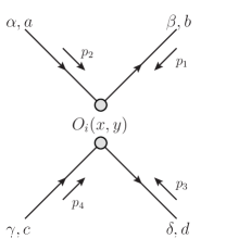
Figure 1: Connected diagram of the generic four-point function described in eq. (6) and fourier transformed with phases $e^{ip_{k}y_{k}}$. Disconnected contributions are forbidden by the flavor structure of the operators $O_{i}$. In our notation the four external quarks have all in-coming momenta.

To compute the quark propagators we invert the Dirac operator $D(x,y)$ on plane waves with momentum $p$ (we later refer to them as momentum sources)

$$G(x,p)=\sum_{y}D^{-1}(x,y)e^{ipy}\,.$$ (7)

By saturating the $x$-dependence with the appropriate phase factor, we obtain the propagator in momentum space and its expectation value

$$\tilde{G}(x,p)=e^{-ipx}G(x,p)\,,$$ (8)

$$S(p)=\frac{1}{V}\sum_{x}\langle e^{-ipx}G(x,p)\rangle\,.$$ (9)

The periodicity of the lattice in the temporal and spatial directions imposes a constraint on the accessible momenta $p_{\mu}=2\pi n_{\mu}/L_{\mu}$, with $n_{\mu}$ a positive integer. Moreover the breaking of the group of continuous rotations to the hypercubic ones leads to additional discretization effects that spoil the smoothness of the propagators as a function of $p$. To overcome both issues we employ twisted boundary conditions (BC) in the valence sector de Divitiis et al. (2004); Boyle (2004); Arthur and Boyle (2011), that allow to access a dense set of momenta

$$p_{\mu}=\frac{2\pi n_{\mu}}{L_{\mu}}+\frac{\theta_{\mu}}{L_{\mu}}\,,\quad\theta_{\mu}\in[-\pi/2,\pi/2]\,.$$ (10)

For simplicity we give below the explicit expression of $\Gamma(O_{2})$, where we omit the index contractions inside the square brackets and where we use the $\gamma_{5}$-hermiticity of the Dirac operator

$$\begin{split}[\Gamma(O_{2})&]^{\alpha\beta\gamma\delta}_{abcd}(p_{1},p_{2},p_{3},p_{4})=\sum_{\mu\nu}\sum_{x,y}\\ &\langle\big{[}\gamma_{5}\tilde{G}(x,-p_{2})^{\dagger}\gamma_{5}\gamma_{\mu}^{L}\tilde{G}(x,p_{1})\big{]}^{\alpha\beta}_{ab}f_{\mu\nu}(x,y)\\ &\times\big{[}\gamma_{5}\tilde{G}(y,-p_{4})^{\dagger}\gamma_{5}\gamma_{\nu}^{L}\tilde{G}(y,p_{3})\big{]}^{\gamma\delta}_{cd}\rangle\,.\end{split}$$ (11)

The amputated amplitudes $\Lambda$ are easily obtained by inverting the expectation value of quark propagators $S(p_{i})$ in eq. (9)

$$\begin{split}[\Lambda(\Gamma)]^{\alpha\beta\gamma\delta}_{abcd}=&[S(p_{2})^{-1}]^{\alpha\alpha^{\prime}}_{aa^{\prime}}[S(p_{1})^{-1}]^{\beta\beta^{\prime}}_{bb^{\prime}}[S(p_{4})^{-1}]^{\gamma\gamma^{\prime}}_{cc^{\prime}}\\ &[S(p_{3})^{-1}]^{\delta\delta^{\prime}}_{dd^{\prime}}\Gamma^{\alpha^{\prime}\beta^{\prime}\gamma^{\prime}\delta^{\prime}}_{a^{\prime}b^{\prime}c^{\prime}d^{\prime}}\,.\end{split}$$ (12)

At this point we define the amputated amplitudes $\Lambda_{i}\equiv\Lambda(\Gamma(O_{i}))$ with $f_{\mu\nu}(x,y)=\delta_{\mu\nu}\delta(x-y)$. On the full theory side, only a single operator with color diagonal structure is needed to describe this process, namely $O_{2}$ in eq. (5) with $f_{\mu\nu}(x,y)=W_{\mu\nu}(x,y)$, the tree-level propagator of the weak charged bosons in coordinate space (Euclidean metric), which we obtain by fourier transforming

$$W_{\mu\nu}(p)=\frac{1}{p^{2}+m_{\mathrm{W}}^{2}}\Big{(}\delta_{\mu\nu}-\frac{p_{\mu}p_{\nu}}{m_{\mathrm{W}}^{2}}\Big{)}\,.$$ (13)

Eqs. (6,11,12) hold in this case as well and we define $\Lambda_{\mathrm{SM}}$ as the amputated amplitude obtained from $O_{2}$ with $f$ replaced by the $W$ boson propagator given above. The choice of the unitary gauge simplifies the calculation in the full theory to a single diagram. In the next section we present results also for the Feynman gauge ($R_{\xi}$ gauge with $\xi=1$) where the contribution of the Goldstone boson needs to be included.

The $\delta(x-y)$ function in the insertion of the local operators $Q_{i}$ simplifies the double sum over $x$ and $y$ in eq. (11) to a single one. Choosing plane waves at the source of the propagators allows us to perform such a sum over the entire volume, thus sampling the operators $Q_{i}$ on the full lattice and reducing the statistical fluctuations of the final amplitudes. When $f$ is replaced by the $W$ boson propagator, the double sum needs to be performed. Also in this case the usage of momentum sources gives us the freedom (at the sink of the propagators) to evaluate both sums over $x$ and $y$ explicitly, thus significantly reducing the noise of $\Lambda_{\mathrm{SM}}$.

The only drawback of the combined use of momentum sources and twisted BCs is that a separate inversion is necessary for each momentum configuration that is considered, up to a total of 4 per configuration if we choose the four external legs with different momenta. Therefore, in an effort to balance the cost of the inversions against the benefit of the volume average, we have explored a second strategy to sample the $W$ boson propagator. From the simple observation that a point-source propagator can be fourier transformed to any continuous momentum, up to small finite-size errors, we have studied the possibility to stochastically sample $W_{\mu\nu}(x,y)$, with $x$ and $y$ being the sources of the inversions rather than the sinks as in the case of momentum sources. The sampling technique is essentially borrowed from the calculation of the light-by-light contribution to the anomalous magnetic moment of the muon by the RBC/UKQCD collaboration Blum et al. (2016a) and it proceeds in two steps:

• for a fixed $x$, the sum over $y$ in eq. (11) is achieved by randomly sampling $W_{\mu\nu}$ with a probability distribution falling off rapidly for large separations $|x-y|$; to recover the flat sum over $y$ the appropriate reweighting factor is applied and to further decrease the cost, the hypercubic symmetries are taken into account by randomly sampling only one element per equivalence class, defined by all the points $y$ with the same distance from $x$, $|x-y|$; this procedure defines a cloud of points stochastically sampled around the center $x$;

• to reduce the noise of the observables a second sum over the center of the cloud, $x$, is performed, which is again stochastic and with a flat distribution.

Even though a continuous set of momenta is now accessible through the usage of the point sources (exceptional and non-exceptional kinematics can also be explored simultaneously), the statistical noise grows quickly: in our test we have used 40 points inside the cloud and this led to a controlled approximation of the sum over $y$ (for the different values of the input $W$ mass considered in this work); however the second sum over $x$, for which we used 16 different clouds, turns out to be the crucial one in further reducing the noise. Although the presence of a finite correlation length in our system decreases the number of useful points to reduce the noise, we have verified that the stochastic sampling leads to results that are at least 10 times noisier compared to the momentum source method, for approximately the same cost. For this reason we leave all the details of this secondary approach to the Appendix A and we concentrate in the rest of the manuscript on the analysis of the results from momentum sources. Nevertheless this technique has been very useful in an early stage of the work when we explored a vast range of momenta and kinematic configurations, on which we based our decision for the final strategy.

II.2 The Wilson coefficients

The appearance of new divergences in the EFT requires the introduction of additional renormalization conditions. In our study we adopt a variety of regularization independent schemes, called RI/MOM and RI/SMOM, which were introduced in Refs. Martinelli et al. (1995); Aoki et al. (2008); Sturm et al. (2009), that are entirely defined by the choice of the external states and projectors: this translates into the momentum combination used in the calculation of the propagators and the projectors that we apply on the amputated Green’s functions to obtain definite spin-color states.

In this paper we have explored two combinations of the four momenta on the external legs: the non-exceptional case called RI/SMOM where $(p_{i}+p_{j})\neq 0$ for all pairs $i\neq j$, and the exceptional one (RI/MOM) where at least one linear combination of the external momenta vanishes. If the amplitude under study possesses the same symmetries of the light mesons, at momenta comparable with their Compton wave length, the smooth perturbative behavior of the amplitude may be spoiled by non-perturbative contaminations, referred to as Goldstone-pole contaminations Martinelli et al. (1995); Aoki et al. (2008). Using non-exceptional kinematics (RI/SMOM) suppresses these unwanted effects Aoki et al. (2008); Sturm et al. (2009) and we extensively discuss them in the next section.

To define specific spin-color states we use two projectors $P_{i}$ ($i=1,2$) that we apply to the amputated amplitudes to define the matrix

$$M_{ij}=\mathrm{Tr}~{}\big{(}P_{j}\Lambda_{i}\big{)}\,,$$ (14)

such that $M$ is invertible. To achieve this we fix the color structure of the projectors to one of the operators

$$P_{1}=\delta_{bc}\delta_{da}\,\Gamma_{1}\otimes\Gamma_{2}\,,\quad P_{2}=\delta_{ba}\delta_{dc}\,\Gamma_{1}\otimes\Gamma_{2}\,,$$ (15)

and we explore two options for the Dirac part, with different parities (even and odd)

$$\Gamma_{1}\otimes\Gamma_{2}=\bigg{\{}\begin{array}[]{lcl}\gamma_{\mu}\otimes\gamma_{\mu}&+&\gamma_{\mu}\gamma_{5}\otimes\gamma_{\mu}\gamma_{5}\\ \gamma_{\mu}\gamma_{5}\otimes\gamma_{\mu}&+&\gamma_{\mu}\otimes\gamma_{\mu}\gamma_{5}\end{array}\,.$$ (16)

Eq. (16) defines the so-called $\gamma$ (or $\gamma_{\mu}$) projectors. Alternatively, the replacement $\gamma_{\mu}\to\not{q}/|q|$ and $\gamma_{\mu}\gamma_{5}\to\not{q}\gamma_{5}/|q|$ defines the $\not{q}$ projectors. Computing the Wilson coefficients using both parities and $\gamma$ or $\not{q}$ Dirac structures turns out to be a crucial test of the calculation, as explained in the next section. In the rest of the paper we will refer to the two parities as $\mathrm{VV}+\mathrm{AA}$ and $\mathrm{VA}+\mathrm{AV}$, with $V$ and $A$ labeling vector and axial Dirac structures.

The renormalization conditions that we impose on the four-quark operators read as follows

$$\lim_{m_{q}\to 0}\ \frac{Z_{ij}^{\mathrm{RI}}}{(Z_{q}^{\mathrm{RI}})^{2}}\,M_{jk}^{\mathrm{lat}}|_{\mu^{2}=p^{2}}=M_{ik}^{\mathrm{RI}}|_{\mu^{2}=p^{2}}\equiv M_{ik}^{\mathrm{tree}}$$ (17)

with

$$Z_{q}^{\mathrm{RI}}S(p)^{\mathrm{lat}}=S(p)^{\mathrm{RI}}\,,$$ (18)

^lat indicating bare lattice quantities and $M_{\mathrm{tree}}$ defined by replacing the amplitudes in eq. (14) with their tree-level counterparts.

In the full theory no additional renormalization conditions are required for the projected amplitude, which we denote with $W_{i}=\mathrm{Tr}~{}(P_{i}\Lambda_{\mathrm{SM}})$, beyond the usual wave function renormalization introduced above. It is important to note that since we are considering the weak theory at tree level, $m_{\mathrm{W}}$ does not renormalize, since self-energy diagrams of the $W$ boson propagator appear at higher orders in the weak coupling constant, $g_{2}$. In the continuum theory, vector and axial current conservations (for mass-less quarks) guarantee that the same is true for $g_{2}$ as well. On the lattice however the usage of local vector and axial currents dictates the presence of the finite renormalization factors $Z_{V}$ and $Z_{A}$, thus leading to $g_{2}^{R}=Z_{V}g_{2}$. Note that the $V-A$ current can be renormalized with either $Z_{A}$ or $Z_{V}$ due to the excellent chiral properties of the Domain Wall formulation and to the employment of non-exceptional kinematics, as described later. Eventually we opt for $Z_{V}$ to avoid additional chiral symmetry breaking effects and a larger quark mass dependence compared to $Z_{A}$.

Now we have all the basic ingredients to impose the matching between the two theories

$$\frac{G_{\mathrm{F}}}{\sqrt{2}}\ C_{i}^{{\mathrm{RI}}}(\mu)M_{ij}^{{\mathrm{RI}}}(\mu)=W_{j}^{{\mathrm{RI}}}(\mu)=\frac{g_{2}^{2}}{8}\frac{Z_{V}^{2}}{(Z_{q}^{\mathrm{RI}})^{2}}W_{j}^{\mathrm{lat}}\,.$$ (19)

We have already simplified the usual CKM factors that appear in the same form on both sides of the equation. The weak coupling constant $g_{2}$ simplifies as well with the Fermi constant $G_{\mathrm{F}}$, leaving only a factor $m_{\mathrm{W}}^{2}$ on the right hand side.

By expanding $M^{\mathrm{RI}}$ and $W^{\mathrm{RI}}$ with their corresponding bare lattice counterparts we obtain the definition of the Wilson coefficients

$$\begin{split}C_{i}^{\mathrm{lat}}\equiv&\ m_{\mathrm{W}}^{2}\Big{(}W_{j}^{{\mathrm{lat}}}[M^{{\mathrm{lat}}}]^{-1}_{ji}\Big{)}\,,\\ C_{i}^{{\mathrm{RI}}}(\mu)=&\ C_{j}^{\mathrm{lat}}\ \Big{(}[Z^{{\mathrm{RI}}}(\mu)]^{-1}_{ji}Z_{V}^{2}\Big{)}\,.\end{split}$$ (20)

Eq. (20) nicely separates two basic ingredients and consequently two different problems:

• the bare lattice Wilson coefficients $C_{i}^{\mathrm{lat}}$ which can be used to inspect the size of the higher dimensional operators and other systematic errors, and that we compute at small momenta for a variety of external states;

• the renormalization factors that we compute at high momenta and use to renormalize $C_{i}^{\mathrm{lat}}$ and eventually connect to the ${\overline{\mathrm{MS}}}$ scheme, by means of the one-loop conversion matrix $Z^{{\mathrm{RI}}\to{\overline{\mathrm{MS}}}}$ given in the Appendix B.

Our analysis proceeds along these two steps: we first examine the dependence of the bare Wilson coefficients on the momentum scale, the quark mass and the finite box size. Then we briefly describe the results for the renormalization matrices and discuss discretization errors, and finally present the comparison against the known perturbative results in the ${\overline{\mathrm{MS}}}$ scheme.

III Results

In our study we have used the Domain Wall formalism, which retains excellent chiral properties, even at finite lattice spacing Blum and Soni (1997a, b) (which become exact in the limit of infinite 5th dimension Shamir (1993); Furman and Shamir (1995)), simplifying the renormalization pattern of the theory and suppressing the mixing among operators belonging to different representations of the chiral group Blum et al. (2003).

We have measured the amplitudes described in the previous section on three different ensembles, reported in Table 1, with 2+1 Domain Wall Fermions (DWF) in the sea. We have used a unitary setup by promoting the same discretization (Shamir DWF) also to the valence sector. Ensembles 16I and 24I have been used to study the dependence of the Wilson coefficients on the volume of the lattice. The additional ensemble 32I allows us to take the continuum limit, with two lattice spacings differing approximately by a factor of 2 in $a^{2}$. In all our calculations we have fixed the (QCD) gauge to the Landau gauge.

Id	$\beta$	$a~{}[\mathrm{GeV}^{-1}]$	$L/a\times T/a$	$am_{\mathrm{u,d}}$	$am_{\mathrm{s}}$
16I	2.13	1.78	$16^{3}\times 32$	0.01	0.04
24I	2.13	1.78	$24^{3}\times 64$	0.01	0.04
32I	2.25	2.38	$32^{3}\times 64$	0.008	0.03

Table 1: List of the ensembles used in this work. In the table we report the most important physical parameters, the remaining details can be found in Refs. Aoki et al. (2011); Allton et al. (2007). The three ensembles have been generated with the same Domain Wall discretization for the sea quarks, the Shamir formulation with fifth dimension length $L_{s}=16$, and Iwasaki gauge action, with bare couplings $g_{0}^{2}=6/\beta$ reported in the second column. In the third column we quote the lattice spacings measured in LABEL:Blum:2014tka and in the last ones we provide the lattice dimensions and the bare sea quark masses.

Our measurements require the calculation of quark propagators for which we have used a mass (in lattice units) of 0.04 on the 24I and 16I ensemble, and 0.03 on the 32I. We utilize 27 independent configurations for both 24I and 32I, separated by 100 and 200 Molecular Dynamics Units. In our analysis we use the jackknife method with bin size of 1, after checking the stability of the error of the Wilson coefficients for larger bin sizes. On our coarser ensembles, the 16I and 24I, we measure our propagators up to momenta of $O(0.8~{}\mathrm{GeV})$, with data points evenly spaced in $p^{2}$. On each configuration we perform 4 different inversions at fixed $p^{2}$ for the four different legs required in non-exceptional kinematics. Moreover on the 16I and 24I we also measure the same amplitudes with momentum injected explicitly along the time direction to test finite volume effects as explained later. On the 24I we repeat those measurements for three values of the quark mass, with $am=0.02\,,0.04$ and 0.08. Finally on the 32I we compute the amplitudes for four different momenta up to $0.4~{}\mathrm{GeV}$. Our calculations of $\Lambda_{\mathrm{SM}}$ cover a range for $am_{\mathrm{W}}$ that goes from $0.6$ to $1.334$ on the 24I and $0.6<am_{\mathrm{W}}<1.0$ on the 32I: the masses on the 32I have been tuned to match those on the 24I according to the ratio of lattice spacings computed in LABEL:Blum:2014tka.

When the momentum of the external quark states becomes comparable to $m_{\mathrm{W}}$, the four-quark EFT is expected to deviate from the full theory, due to the lack of higher dimensional operators that eventually become relevant. Therefore for different choices of the external states in our definition of the amplitudes, we expect to observe different behaviors with respect to the dominant scale $p^{2}$. However, in the limit where $p^{2}/m_{\mathrm{W}}^{2}\ll 0$ they should all agree and give a consistent and unique value for the Wilson coefficients, up to $O(\Lambda_{\mathrm{QCD}})$ contributions. This suggests that we should be able to fit $C_{i}^{\mathrm{lat}}$ with a polynomial function of $p^{2}/m_{\mathrm{W}}^{2}$ and we turn to this now. In the next sections we address the problems related to the usage of small momenta such as finite volume and finite quark mass effects and possible remaining non-perturbative effects of order $\Lambda_{\mathrm{QCD}}/m_{\mathrm{W}}$.

III.1 Fitting strategy

In order to address the size of higher dimensional operators we study the momentum dependence of the $C_{i}^{\mathrm{lat}}$s for several choices of the external states: we adopt a non-exceptional momentum configuration given by

$$\begin{split}p_{1}=(x,-x,0,0)\quad p_{2}=(0,0,-x,x)\\ p_{3}=(-x,0,x,0)\quad p_{4}=(0,x,0,-x)\end{split}$$ (21)

with $p_{i}^{2}=p^{2}$, $\forall i$, and transfer momentum $q^{2}=2p^{2}$. In eq. (21) $x$ denotes a continuous parameter obtained according to eq. (10). The exceptional momentum configuration is easily obtained by re-using the same propagator with one of the four momenta in eq. (21) on all the four legs. The momentum configuration proposed in eq. (21) leads to momentum conservation in the amplitudes and to exact equivalence between $\gamma$ and $\not{q}$ projectors.

Figure 2: Dependence of the bare lattice Wilson coefficients on the momentum of the external quark states for a fixed value of $m_{\mathrm{W}}\approx 1.8~{}\mathrm{GeV}$. The two sets of data points correspond to the exceptional and non-exceptional kinematics described in eq. (21) measured on the 24I ensemble with $am=0.04$. We perform combined polynomial fits where the constant term is constrained by the two data sets, which have been obtained from $\not{q}$ parity odd projectors.

In Figure 2 we show the results of $C_{1}^{\mathrm{lat}}$ and $C_{2}^{\mathrm{lat}}$ as a function of $p^{2}/m_{\mathrm{W}}^{2}$ from the 24I ensemble. We observe a good convergence of the two sets of data points (exceptional and non-exceptional) for small values of the expansion variable $p^{2}/m_{\mathrm{W}}^{2}$. Nevertheless higher dimensional operators are quite sizable, given the high accuracy that we are able to achieve, which forces us to explore a particularly small range of momenta and eventually consider extrapolations to $p^{2}/m_{\mathrm{W}}^{2}\to 0$. However, data obtained with non-exceptional kinematics show a milder dependence on the external momentum $p^{2}$.

To extract the bare values of the Wilson coefficients showed in Figure 2, we adopt combined polynomial fits to the exceptional and non-exceptional points with a common constant term

$$\begin{split}C_{i}^{{\mathrm{lat}},\mathrm{ex}}(x)&=C_{i}^{\mathrm{lat}}+\sum_{k=1}^{N}A_{ik}x^{k}\,,\quad i=1\,,2\\ C_{i}^{{\mathrm{lat}},\mathrm{nonex}}(x)&=C_{i}^{\mathrm{lat}}+\sum_{k=1}^{N}B_{ik}x^{k}\,,\quad x=\frac{p^{2}}{m_{\mathrm{W}}^{2}}\,.\end{split}$$ (22)

We base our decision for a combined fit on the fact that independent fits to the two data sets reproduce results for $C_{i}^{\mathrm{lat}}$ well compatible within 1 standard deviation (on a given fit range). To estimate the systematic uncertainties associated with these extrapolations we vary the upper limit of the fit range and the degree of the polynomial ($N=1,2,3$) and we consider the fits with good $\chi^{2}$ per d.o.f: we take as our final value the result from the highest polynomial, whose larger statistical error covers the discrepancy among the several fits.

With the lattice spacings that we have studied in this work, higher dimensional operators seems to be sufficiently suppressed only for momenta around and below $\Lambda_{\mathrm{QCD}}$. Therefore studying the dependence on the infrared regulators of the lattice Wilson coefficients is important to control their extraction. In general we expect them to be small in $C_{i}^{\mathrm{lat}}$ due to their cancellation between $W$ and $M$, especially if the quark momentum is well below $m_{\mathrm{W}}$. However to what degree this is realized in practical non-perturbative simulations is not clear a priori and we study that below.

III.2 Finite Volume Errors

The first infrared regulator that we investigate is the box size. For this purpose we have measured the lattice Wilson coefficients on the 16I and 24I ensembles using exceptional kinematics. In Figure 3 we present the results for $C_{2}^{\mathrm{lat}}$: note that the two plots, corresponding to the two ensembles, share the same y-axis to facilitate a visual comparison. Both plots contain four sets of points obtained by combining $\gamma$ and $\not{q}$ projectors with amplitudes where the momentum is injected along $xy$ and time directions. The parity of the projectors corresponds to $\mathrm{VA}+\mathrm{AV}$.

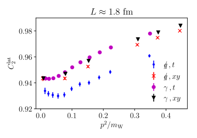
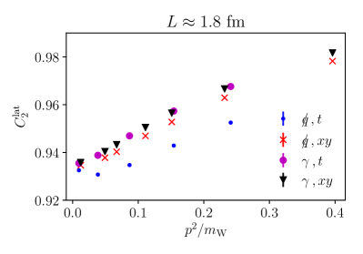
Figure 3: Dependence of the lattice Wilson coefficient $C_{2}^{\mathrm{lat}}$ on the momentum of the external states for fixed $m_{\mathrm{W}}\approx 1.8~{}\mathrm{GeV}$. The labels in the legend denote the choice of projectors ($\gamma$ or $\not{q}$) and momentum (injected along $xy$ spatial directions or time $t$). Both panels show points obtained from parity odd projectors. Left: results from the 16I ensemble; if the momentum is along the time direction, twice as big as the spatial ones, $C_{2}^{\mathrm{lat}}$ from $\not{q}$ projectors coincides with the measurements performed on the larger lattice. Right: results from the 24I ensemble where all combinations of momentum and projectors converge to the same point in the limit of small momenta.

For the 24I ensemble the various measurements converge to a unique point at small momenta, thus remarking the universality of the Wilson coefficients in that limit. However for the 16I ensemble a different behavior is observed: in this case only the combination of $\not{q}$ projectors with amplitudes with momentum along the time direction agrees with the correponding measurements in the larger volume, while the other sets of points converge to a different value. We interpret such a behavior as a finite volume error, that is largely suppressed when the momentum is injected along the time direction, which is twice as big as the spatial ones. From our numerical analysis we have noticed that the finite volume effect measured in the 16I ensemble decreases with $m_{\mathrm{W}}^{-1}$. In agreement with other observations presented later, this may be a consequence of a dimension-7 operator involving a non-perturbative condensate, whose strong dependence on the box volume eventually generates the spread that we observed.

A similar behavior is observed also in the other Wilson coefficient, $C_{1}^{\mathrm{lat}}$, where the measurements on the 16I do not agree at small momenta, in constrast with the 24I ensemble.

III.3 Non-perturbative effects

In our study we have not been able to achieve a large separation between the strong and weak scales, since $\Lambda_{\mathrm{QCD}}/m_{\mathrm{W}}\approx 0.2$. This means that our calculation, based on RI/MOM techniques, might potentially suffer from non-perturbative contaminations often referred to as Goldstone-pole contaminations Martinelli et al. (1995); Aoki et al. (2008): in general varying the quark mass in the measurements of the amplitudes is useful to address this issue and has been previously used to non-perturbatively subtract them away Becirevic et al. (2004). Such contaminations are present mostly in observables that share the same quantum numbers of the lighter mesons, such as the axial or pseudo-scalar bilinear operators (see for example LABEL:Giusti:2000jr). If we extend the discussion to fermionic formulations that do not preserve chiral symmetry, such as Wilson fermions, also the mixing with wrong chiralities is allowed and at small momenta can lead to pole behavior as well. For our study we have checked how well chiral symmetry is realized by repeating some measurements of the Wilson coefficients with a larger separation of the Domain Walls along the fifth dimension: we have obtained an excellent agreement for all combinations of projectors between results obtained with the Shamir formulation with $L_{s}=32$ and $L_{s}=16$ (the latter being the same one used for the sea quarks). Hence, we expect any mixing with wrong chiralities to be predominantly of infrared origin, due to the spontaneous breaking of chiral symmetry via quark condensates, and to vanish at high momenta. Based on $\mathcal{CPS}$ symmetry arguments Bernard et al. (1985, 1988); Donini et al. (1999), we also expect the parity odd projectors to show less contaminations compared to the parity even case.

Figure 4: Quark mass dependence of $C_{2}^{\mathrm{lat}}$ for fixed input $W$ mass at $1.8~{}\mathrm{GeV}$ on the 24I ensemble. Crosses refer to parity even projectors and dots represent the opposite parity, all in the $\gamma$ scheme. No difference is observed if $\gamma$ projectors are replaced with the corresponding $\not{q}$ ones. The $\mathrm{VV+AA}$ projectors produce results very sensitive to the quark mass, contaminated by infrared effects proportional to $1/p^{2}$. A small quark mass dependence is observed in $C_{1}^{\mathrm{lat}}$ for parity odd projectors as well.

To quantify this problem we start from the difference between the Wilson coefficients computed with parity even and parity odd projectors, defined in eq. (16), for several values of the valence quark mass. In Figure 4 we show the results for the lattice Wilson coefficient $C_{2}^{\mathrm{lat}}$ from the exceptional momentum configuration, where we vary the quark mass and the parity of the ($\gamma$) projectors used to compute $M^{\mathrm{lat}}_{ij}$ and $W_{i}^{\mathrm{lat}}$. For parity odd projectors we observe an excellent agreement among the different quark masses for all points, down to the smallest momentum. On the other hand parity even projectors lead to a strong dependence of $C_{2}^{\mathrm{lat}}$ on the quark mass, well compatible with the expectation of a Goldstone-pole contamination: in fact, by increasing the quark mass from 0.02 to 0.08 the data is driven towards the points obtained from parity odd projectors, due to the suppression of non-perturbative effects which we expect to be proportional to $(p^{2}+m^{2})^{-1}$, with $m$ the mass of the light state coupling to the amplitude. Changing from $\gamma$ to $\not{q}$ projectors does not affect the general trend showed in Figure 4, as well as turning to the non-exceptional kinematics in eq. (21). For $C_{1}^{\mathrm{lat}}$ we draw similar conclusions on the behavior of the parity even results, with the only exception that a quark mass depedence is visible also for parity odd projectors: given the different nature and size of this Wilson coefficient it turns out to be large, on the 10% level, but only 0.015 in absolute units (with $C_{1}^{\mathrm{lat}}\approx 0.15$). We account for this effect in our systematic error.

To better understand the origin of the discrepancy between the two parities, we have projected our amputated Green’s functions on the so-called wrong chiralities. For odd parity no significant mixing has been found. Instead we have measured strong contributions at small momenta from the projectors with form $1\otimes 1$, $\gamma_{5}\otimes\gamma_{5}$ and $\sigma_{\mu\nu}\otimes\sigma_{\mu\nu}$, which quickly vanish above $1~{}\mathrm{GeV}$. This provides another indication on the pollution of infrared effects in the parity even sector, as expected from $\mathcal{CPS}$ symmetry. In Appendix C we describe an alternative approach consisting of changing the definition of the projectors to suppress the overlap with the unwanted chiralities.

Checking the gauge independence of our calculation is a second approach that we exploit to quantify non-perturbative contributions of $O(\Lambda_{\mathrm{QCD}})$. Specifically, we have computed the $W_{i}^{\mathrm{lat}}$ amplitudes in Feynman gauge. In this case the weak boson propagator simplifies to the diagonal form

$$W_{\mu\nu}=\frac{\delta_{\mu\nu}}{p^{2}+m_{\mathrm{W}}^{2}}$$ (23)

but the amplitude, even at tree-level, requires also the contribution of the Goldstone boson arising after the Electro-Weak Symmetry Breaking.

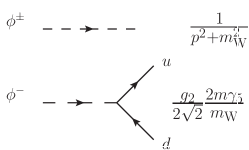
Figure 5: Goldstone boson propagator and coupling to the quark current. In the latter we have already assumed degenerate quark masses and simplified the contribution proportional to the identity.

In our case, where all the external legs have the same mass, the vertex between the Goldstone and two quarks simplifies to the form reported in Figure 5. In the limit of mass-less quarks it should vanish identically thus leaving only eq. (23) to contribute to the amplitude. This may be spoiled again by non-perturbative effects, which may be very pronounced due to the $\gamma_{5}\otimes\gamma_{5}$ structure of this diagram. Therefore studying the two contributions separately could shed some light on the size of these effects and we examine this in Figure 6, which shows the Wilson coefficients $C_{i}^{\mathrm{lat}}$ computed only from the Goldstone boson diagram and with parity even projectors. Note that the full Wilson coefficients are obtained simply by adding the result of Figure 6 to the $C_{i}^{\mathrm{lat}}$s computed from the $W$ exchange alone.

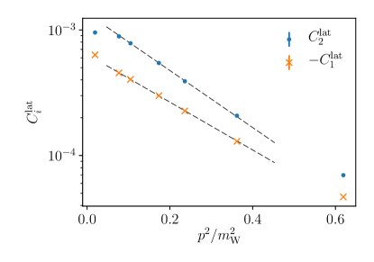
Figure 6: Contribution of the Goldstone boson exchange to the Wilson coefficients with parity even $\gamma$ projectors. The two lines are linear fits of $\log C_{i}^{\mathrm{lat}}$ in $p^{2}/m_{\mathrm{W}}^{2}$, which describe well the data. The suppression given by the prefactor in the vertices, $(2m/m_{\mathrm{W}})^{2}=0.0064$, makes the two contributions negligible, even though they slightly reduce the discrepancy from the $C_{i}^{\mathrm{lat}}$s obtained with parity odd projectors.

For parity odd projectors the contribution from the Goldstone boson is negligible, numerically below $10^{-6}$ and compatible with zero within 1 sigma. For parity even projectors, in contrast, we can measure a signal from the Goldstone boson diagram. However the small prefactor $(2m/m_{\mathrm{W}})^{2}$ makes this contribution negligible also in this case, as plotted in Figure 6, although it moves both $C_{1}^{\mathrm{lat}}$ and $C_{2}^{\mathrm{lat}}$ towards the corresponding parity odd data.

Next we compare the Wilson coefficients measured in Unitary and Feynmann gauge with odd projectors exclusively, for which the Goldstone boson diagram can be neglected. The difference that we observe between the sets of data points comes from the gauge depedent part of the weak propagator in eq. (13) proportional to $p_{\mu}p_{\nu}$. The dependence on the weak gauge fixing condition is expected to vanish for on-shell quantities, which we approach by injecting smaller and smaller momenta in the external quark legs of our amplitudes. As seen already above, in this limit non-perturbative effects produce contaminations that in this case let gauge-dependent terms survive: results between Feynman and Unitary gauge do not agree at the 2% level, even for the preferred parity odd projectors, and we may consider this difference as one source of systematic uncertainties $\delta C_{i}^{\mathrm{gauge}}(m_{\mathrm{W}}\,,p^{2})=|C_{i}^{{\mathrm{lat}},\mathrm{unit}}(m_{\mathrm{W}}\,,p^{2})-C_{i}^{{\mathrm{lat}},\mathrm{feyn}}(m_{\mathrm{W}}\,,p^{2})|$.

However, a second systematic error that we include in our calculation is taken from the difference between the even and odd projectors in Unitary gauge, $\delta C_{i}^{\mathrm{proj}}=|C_{i}^{{\mathrm{lat}},\mathrm{VV+AA}}-C_{i}^{{\mathrm{lat}},\mathrm{VA+AV}}|$ (for better readability we omit the $m_{\mathrm{W}}$ and $p^{2}$ dependence). The latter turns out to be much larger than $\delta C_{i}^{\mathrm{gauge}}$ and similarly accounts for non-perturbative contaminations. Therefore we have decided to discard $\delta C_{i}^{\mathrm{gauge}}$.

Finally we also consider the quark mass dependence as a source of systematic uncertainties, $\delta C_{i}^{\mathrm{mass}}=|C_{i}^{{\mathrm{lat}},am=0.04}-C_{i}^{{\mathrm{lat}},am=0.02}|$, measured for exceptional kinematics only from parity odd projectors.

Now that we have established how to quantify remaining non-perturbative effects, as our last step in the extraction of the Wilson coefficients we study the dependence of the total systematic uncertainty on the lower end ($p_{\mathrm{cut}}$) of the fit range of $C_{i}^{\mathrm{lat}}$

$$\delta C_{i}^{\mathrm{lat}}(p_{\mathrm{cut}})=\sqrt{(\delta C_{i}^{\mathrm{proj}})^{2}+(\delta C_{i}^{\mathrm{mass}})^{2}+(\delta C_{i}^{\mathrm{poly}})^{2}}\,,$$ (24)

where we also quote the extrapolation error $\delta C_{i}^{\mathrm{poly}}$ as a function of $p_{\mathrm{cut}}$ by taking the difference of the intercepts of two different polynomial fits.

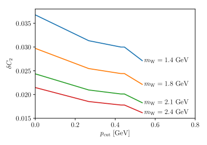
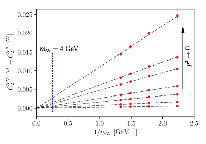
Figure 7: Left: $\delta C_{2}$, as a function of $p_{\mathrm{cut}}$, decreases as more points at small momenta are excluded from the fit, suppressing non-perturbative effects. Right: measured difference of $C_{2}$ from odd and even projectors in the $\gamma$ scheme as function of the $W$ boson mass. The lines are linear fits forced to pass through the origin with excellent $\chi^{2}$. The non-perturbative contaminations which we quantify with $\delta C_{i}^{\mathrm{proj}}$ given in eq. (24) seem to vanish only with one inverse power of $m_{\mathrm{W}}$. In the plot we present the data for the exceptional kinematics, but practically no difference is observed in the non-exceptional case.

In general, all the systematic uncertanties quoted in eq. (24) are estimated from the combined fits defined in eq. (22) where we exclude the points with $p^{2}<p_{\mathrm{cut}}^{2}$. As we increase $p_{\mathrm{cut}}$ in our fit ranges, $\Lambda_{\mathrm{QCD}}$-type contributions are expected to vanish and this is reflected by our systematic uncertainty, which decreases also for larger values of $m_{\mathrm{W}}$. We demonstrate both behaviors in the two panels of Figure 7: the left one confirms essentially the left-most inequality in eq. (3) and the fact the natural variable to control non-perturbative effects is precisely $p_{\mathrm{cut}}$; the right plot also confirms the general expectation that uncertainties are reduced with a larger separation between the ${\mathrm{QCD}}$ and weak scales. An additional indication of the non-perturbative origin of these contributions resides in the linear behavior in $1/m_{\mathrm{W}}$ showed in Figure 7: the presence of a condensate (a pure non-perturbative effect) could be captured by a higher dimensional operator in the form of

$$\frac{\bar{q}q}{p^{2}m_{\mathrm{W}}}O^{(6\mbox{-}\mathrm{dim})}\,,$$ (25)

whose functional form describes well the data.

To summarize, we have collected evidence, from the spread between different projectors and gauge fixing conditions to the volume dependence, that lead to infrared contaminations vanishing with $1/m_{\mathrm{W}}$. In the right plot of Figure 7 we also demonstrate how a future calculation with $m_{\mathrm{W}}\approx 4~{}\mathrm{GeV}$ would significantly improve the precision well below the percent level.

Finally, for the central values of the Wilson coefficients we use a $p_{\mathrm{cut}}$ of $0.3~{}\mathrm{GeV}$ for the 24I ensemble and $0.24~{}\mathrm{GeV}$ for the 32I ensemble and we perform cubic and quadratic fits respectively according to eq. (22). We use amplitudes computed in unitary gauge projected on the odd sector with $\not{q}$ type projectors. No significant effect, beyond the ones already considered, is obtained from the difference with $\gamma$ projectors.

IV Non-perturbative determination of the Wilson coefficients

The remaining systematic uncertanties that we need to address are related to discretization errors for which we need the renormalization factors. In the following we present non-perturbative results for the following values of the $W$ boson mass: 1.4, 1.8, 2.1 and 2.4 $\mathrm{GeV}$.

IV.1 Renormalization factors

As before twisted boundary conditions turn out to be very useful, as they give us the possibility to tune the momentum to the desidered value. In our computation of the renormalization factors we have adopted the conventional RI/SMOM scheme described in LABEL:Lehner:2011fz. Here a momentum $2p$ leaves the operator, as opposed to eq. (21), and only two inversions per configuration are required with momentum $p_{1}=(x,-x,0,0)$ and $p_{2}=(0,x,-x,0)$ (with $p_{3}=p_{1}$ and $p_{4}=p_{2}$). Since the renormalization conditions in eq. (17) are imposed in the chiral limit we repeated the measurements for two values of the quark mass ($am=0.04$ and 0.02) and we extrapolate linearly to zero quark masses. We computed the quark propagators such that $|ap|\approx am_{\mathrm{W}}$, to obtain the Wilson coefficients renormalized at a scale coinciding with the mass of the weak boson utilized in their definition: in this way we are reproducing the so-called initial conditions, where large logarithms are avoided as explained in section II.

Finally, we deal with the renormalization of the local currents on the lattice. Therefore from the same set of propagators we also compute the following quantities

$$\begin{split}\Gamma^{V}_{\mu}=&\sum_{x}\langle\gamma_{5}\tilde{G}(x,-p_{2})^{\dagger}\gamma_{5}\ \gamma_{\mu}\ \tilde{G}(x,p_{1})\rangle\,,\\ \Gamma^{A}_{\mu}=&\sum_{x}\langle\gamma_{5}\tilde{G}(x,-p_{2})^{\dagger}\gamma_{5}\ \gamma_{\mu}\gamma_{5}\ \tilde{G}(x,p_{1})\rangle\,.\end{split}$$ (26)

After the usual amputation with the inverse propagators, we impose the renormalization conditions

$$\lim_{m_{q}\to 0}\frac{Z_{V}}{Z_{q}^{\mathrm{RI}}}\mathrm{Tr}~{}[\Lambda_{\mu}^{V}\gamma^{\mu}]=\mathrm{Tr}~{}[\Lambda_{\mu}^{V,{\mathrm{tree}}}\gamma^{\mu}]\,,$$ (27)

$$\lim_{m_{q}\to 0}\frac{Z_{A}}{Z_{q}^{\mathrm{RI}}}\mathrm{Tr}~{}[\Lambda_{\mu}^{A}\gamma^{\mu}\gamma_{5}]=\mathrm{Tr}~{}[\Lambda_{\mu}^{A,{\mathrm{tree}}}\gamma^{\mu}\gamma_{5}]\,.$$ (28)

In principle the appropriate renormalization condition should involve the $\Gamma^{V-A}_{\mu}$, obtained by replacing $\gamma_{\mu}$ with $\gamma_{\mu}^{L}$ in the first line of eq. (26). However we have explicitly checked from our measurements that $\mathrm{Tr}~{}[\Lambda_{\mu}^{A}\gamma^{\mu}]\ll 10^{-3}$ (the same holds if $A\to V$ and $\gamma^{\mu}\to\gamma^{\mu}\gamma_{5}$) which means that for the choice of projectors in eqs. (27,28) only $Z_{V}$ alone (or $Z_{A}$) renormalizes the weak coupling $g_{2}$, thus leading to eq. (19). Replacing $\gamma_{\mu}\to(\not{q}q_{\mu})/q^{2}$ and $\gamma_{\mu}\gamma_{5}\to(\not{q}\gamma_{5}q_{\mu})/q^{2}$ in eqs. (27,28) defines the $\not{q}$ scheme as before. For simplicity, we do not combine $Z_{q}$ and the four-quark $Z$ matrix from two schemes.

Let us briefly examine the properties of the renormalization factor of the Wilson coefficients in eq. (20)

$$\tilde{Z}^{{\overline{\mathrm{MS}}},{\mathrm{RI}}}\equiv Z_{V}^{2}[Z^{\mathrm{RI}}]^{-1}[Z^{{\mathrm{RI}}\to{\overline{\mathrm{MS}}}}]^{-1}\,,$$ (29)

which we explicitly expand in terms of lattice observables for the reader’s convenience (in the $\gamma$ scheme)

$$Z_{V}^{2}[Z^{\mathrm{RI}}]^{-1}_{ik}=\left(\frac{\mathrm{Tr}~{}[\Lambda_{\mu}^{V,{\mathrm{tree}}}\gamma^{\mu}]}{\mathrm{Tr}~{}[\Lambda_{\mu}^{V}\gamma^{\mu}]}\right)^{2}\cdot M^{\mathrm{lat}}_{ij}[M^{\mathrm{tree}}]^{-1}_{jk}\,.$$ (30)

Firstly the quark mass dependence is negligible, as the four elements of the matrix $\tilde{Z}$ slightly differ when the quark mass is changed from 0.04 to 0.02. Nevertheless we take this into account by linearly extrapolating to the chiral limit. Secondly we examine the difference between the renormalization matrix $\tilde{Z}$ computed from two intermediate schemes, defined by the two classes of projectors, $\gamma$ and $\not{q}$. As we change the renormalization scale from 1.4 to 2.4 $\mathrm{GeV}$ the conversion factor $Z^{{\mathrm{RI}}\to{\overline{\mathrm{MS}}}}$, which is only perturbative, becomes more precise. Nonetheless the ratio $\tilde{Z}^{{\overline{\mathrm{MS}}},\gamma}[\tilde{Z}^{{\overline{\mathrm{MS}}},\not{q}}]^{-1}$ significantly deviates from the identity matrix, the signature of missing terms of size $\alpha_{s}^{2}$. The largest departures from 1 are observed in the diagonal terms, specifically from 23 to 18% for the $(1,1)$ element (that contributes mostly to $C_{1}^{\overline{\mathrm{MS}}}$), and from 5 to 4% for the $(2,2)$ element that defines $C_{2}^{\overline{\mathrm{MS}}}$. These higher order effects are relatively large and can be reduced only by pushing the calculation to higher renormalization scales, where $\alpha_{s}$ becomes smaller. Thirdly, at these relatively high momenta, both parity even and odd projectors give results well compatible with each other.

IV.2 Discretization Errors

The lattice cutoff is the main limitation of the current results preventing the weak boson mass from being well separated from lower ${\mathrm{QCD}}$ scales. As we increase it, larger discretization errors are expected and values of $m_{\mathrm{W}}$ of the order of the cutoff may sound already dangerous: in Figure 8 we demonstrate that the parameter space explored in this work is still in a region where discretization errors are reasonably under control.

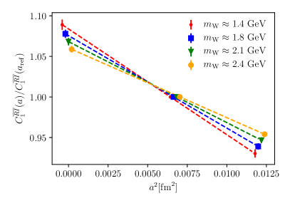
Figure 8: Relative continuum extrapolations of $C_{1}^{\mathrm{RI}}$, renormalized at the value of the $W$ boson mass used to compute them. We normalize the y-axis with the measurement of $C_{1}^{\mathrm{RI}}$ from 32I. The slope of the extrapolations slightly changes with $m_{\mathrm{W}}$, but remains a subdominant effect. The points have been horizontally displaced for better visibility.

By plotting the continuum extrapolations of $C_{1}^{\mathrm{RI}}$ for the four values of $m_{\mathrm{W}}$ considered and normalized at the finer ensemble 32I, we show how the size of the $a^{2}$ coefficient slightly changes with $m_{\mathrm{W}}$, making the $m_{\mathrm{W}}$-dependence practically negligible compared to the overall size of cutoff effects. The scaling violations that we observe for $C_{1}^{\mathrm{RI}}$ range from 10 to 17%; instead they are only at 1% level for $C_{2}^{\mathrm{RI}}$, where the differences among the several values of $m_{\mathrm{W}}$ are also irrelevant. The different magnitudes can be easily understood from the fact that in the free theory $C_{1}=0$ and $C_{2}=1$, meaning that discretization errors start at order $\alpha_{s}$, which on our lattices is approximately 0.3. Nevertheless we perform extrapolations in $a^{2}$ rather than $\alpha_{s}(a)a^{2}$, since the numerical change is irrelevant.

IV.3 Final results and discussions

The last aspect of our work consists of changing renormalization scheme from ${\mathrm{RI}}$ to the more common ${\overline{\mathrm{MS}}}$. This is the only step where perturbation theory enters in our calculation since the conversion matrices are known to 1-loop and reported in Appendix B. In Figure 9 we plot our results together with the known 1-loop analytic formulae that we take from LABEL:Buchalla:1995vs. For the latter we use $\alpha_{s}$ from the 1 and 4-loop $\beta$ function with 3 flavors and $\Lambda^{\overline{\mathrm{MS}}}_{N_{\mathrm{f}}=3}=341(12)\mathrm{MeV}$ taken from LABEL:Bruno:2017gxd. The error from the $\Lambda$ parameter is propagated to the analytic Wilson coefficients and it is represented by the two shaded regions.

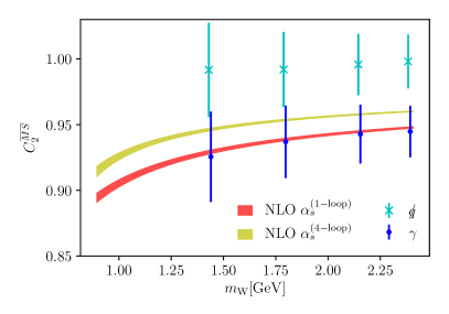
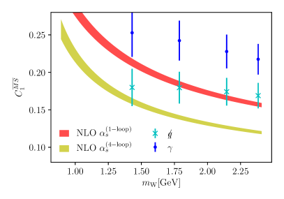
Figure 9: Results in the continuum limit for 3-flavor QCD of the Wilson coefficients in the ${\overline{\mathrm{MS}}}$ scheme as a function of the $W$ boson mass. The shaded regions represent the perturbative one-loop result with error propagated from the $\Lambda$-parameter. The difference between the two intermediate ${\mathrm{RI}}$ schemes accounts for higher order effects in the ${\mathrm{RI}}\to{\overline{\mathrm{MS}}}$ conversion factors. The plotted error bars include both statistical and systematic uncertainties. The latter dominate and gradually decrease with $m_{\mathrm{W}}$.

The non-perturbative results include the various systematic errors described in the previous sections. The systematic uncertainty associated with the perturbative error of the ${\mathrm{RI}}\to{\overline{\mathrm{MS}}}$ conversion, which is an $O(\alpha_{s}^{2})$ effect, can be read off from the difference between the two intermediate ${\mathrm{RI}}$ schemes studied in the paper, the $\gamma$ and $\not{q}$ scheme. Such a difference turns out to be relatively large, following the previous discussion on the renormalization matrix $\tilde{Z}$. We remark that the ${\mathrm{RI}}\to{\overline{\mathrm{MS}}}$ conversion matrix for the $\not{q}$ scheme given in Appendix B contains a large one-loop coefficient, whereas the $\gamma$ scheme shows a much better convergence with a very small correction from ${\mathrm{RI}}$ to ${\overline{\mathrm{MS}}}$.

In Figure 9 we compare our results for the $C_{i}^{\overline{\mathrm{MS}}}$s against the perturbative ones as a function of the $W$ mass. Recall that we are focusing on the initial conditions of the Wilson coefficients, which means that their renormalization scale coincides with $m_{\mathrm{W}}$. The discrepancy between our values and the 1-loop results decreases for larger values of the weak mass as expected from the running of the strong coupling constant, since the perturbative expansion of the Wilson coefficients reads

$$C_{i}(m_{\mathrm{W}})=\sum_{n=0}^{N}\alpha_{s}^{n}(m_{\mathrm{W}})k^{(i)}_{n}+O(\alpha_{s}^{N+1})$$ (31)

with tree-level values $k_{0}^{(1)}=0$ and $k_{0}^{(2)}=1$. The systematic uncertainties plotted in Figure 9 are all correlated with each other, allowing us to fit the data with eq. (31) and still be able to estimate the one-loop coefficients: from the $\gamma$ intermediate scheme alone we obtain $k_{1}^{(1)}=0.64(21)$ and $k_{1}^{(2)}=-0.158(78)$, that agree within 1 sigma with the analytic results taken from LABEL:Buchalla:1995vs, 0.44 and -0.15 respectively.

Given the limitations of the ${\mathrm{RI}}\to{\overline{\mathrm{MS}}}$ conversion factor to one-loop, even with higher precision, fitting our ${\overline{\mathrm{MS}}}$ results beyond $O(\alpha_{s})$ would be incorrect. In fact, we turn now to our non-perturbative determination by sticking to the ${\mathrm{RI}}$ scheme, where we can convert the analytic results of the Wilson coefficients without loss of generality. In Table 2 we report various results from different polynomial fits to the $\gamma$ scheme, following eq. (31), which we also augumented with a term $k_{\Lambda}/m_{\mathrm{W}}$.

$C_{i}^{\mathrm{RI}}$	$k_{1}^{(i)}$	$k_{2}^{(i)}$	$k_{\Lambda}^{(i)}$
1	0.643(60)	—	—
1	1.270(45)	-1.28(0.18)	—
1	0.123(13)	—	0.337(91)
2	-0.158(61)	—	—
2	-0.223(24)	0.01(0.28)	—
2	-0.006(22)	—	-0.14(11)

Table 2: In the first lines we report results for the Wilson coefficient $C_{1}$, whereas the last ones refer to $C_{2}$. All fits have very small $\chi^{2}$ per $\mathrm{d.o.f.}$ due to the large systematic errors. The errors quoted in the table are both statitstical and systematic. In our fits we always use all the four values of $m_{\mathrm{W}}$ explored in this work.

The coefficients reported in Table 2 could be used, in principle, to provide an estimate of the Wilson coefficients for physical values of $m_{\mathrm{W}}$ by using eq. (31) with $\alpha_{s}$ computed at $80~{}\mathrm{GeV}$. With the current large systematic uncertainty we are only sensitive to the 1-loop coefficient, but the results in Table 2 show the potential of the method: the possibility to extract higher loop coefficients can be used to bound the error of $C_{i}(80~{}\mathrm{GeV})$ by considering, for example, the difference between the known 1-loop result and our 2-loop prediction. This approach has the potential to reduce the current systematic uncertainties where these Wilson coefficients are used and are relevant, such as the real part of the amplitudes of $K\to\pi\pi$ for isospin 0 and 2 channels. One caveat that we need to remember is that any prediction of coefficients beyond one-loop depends on the number of flavors used in the simulations. For this reason we intend to continue our study by reusing the methodology developed in this paper on the finer ensembles generated by the RBC/UKQCD Collaboration Frison et al. (2015) with 3 and 4 active flavors in the sea. Such a calculation will provide multiple benefits, from the possibility to push $m_{\mathrm{W}}$ up to 4 $\mathrm{GeV}$ and substantially reduce the systematic uncertainties (see Figure 7), to controlling the flavor dependence of the coefficients of higher loops and reducing the systematic error from intermediate ${\mathrm{RI}}$ scheme, thus providing a solid prediction in the ${\overline{\mathrm{MS}}}$ scheme. Finally, future extensions of this work will include the top quark contribution.

V Conclusions

In this paper we have presented a method to compute the initial conditions of the Wilson coefficients to all orders in the strong coupling constant and leading order in $g_{2}$. We have described the limitations of our exploratory study, mostly related to the presence of large infrared and non-perturbative effects. By looking at different observables we quantified those effects and took them into accout in our systematic uncertainties, that dominate the final errors.

Nevertheless, we have demonstrated how precise statistical results can be achieved with the combined use of momentum sources and twisted boundary conditions. Therefore we expect to obtain excellent results with the next iteration of this calculation repeated on finer lattices, where the systematic errors will significantly decrease.

Despite the limitations imposed by the lattice cutoff, we observed reasonable scaling violations for the values of $m_{\mathrm{W}}$ that we explored. Moreover we discussed a strategy to extend the relevance of our study to place a bound on the error of the Wilson coefficients for the physical scenario with $m_{\mathrm{W}}\approx 80~{}\mathrm{GeV}$.

VI acknowledgements

We would like to thank our RBC and UKQCD collaborators for helpful discussions and support. M.B. is particularly indebeted to N. Christ for a critical reading of the manuscript and to T. Izubuchi and P. Boyle for many stimulating discussions. Computations for this work were carried out at the Fermilab cluster pi0 as part of the USQCD Collaboration, which is funded by the Office of Science of the U.S. Department of Energy. M.B., C.L. and A.S. were supported by the United States Department of Energy under Grant No. DE-SC0012704. In addition C.L. is supported in part through a DOE Office of Science Early Career Award.

Appendix A Stochastic sampling of the weak propagator

In this Appendix we present further details on the alternative stochastic sampling method for the $W$ boson propagator described in the main text. The key ingredient is the possibility to approximate the propagator in momentum space $\sum_{x}e^{ip(y_{0}-x)}D^{-1}(x,y_{0})$ with point-source propagators transformed to any continuous momentum, up to finite-size errors

$$\begin{split}&S^{\mathrm{app}}(p)=\sum_{x}D^{-1}(x,y_{0})\\ &\times\left\{\begin{array}[]{ll}e^{ip_{\mu}(y_{0}-x)_{\mu}}&|y_{0}-x|_{\mu}<L_{\mu}/2\\ e^{ip_{\mu}(y_{0}-x+L)_{\mu}}&(y_{0}-x)_{\mu}\leq-L_{\mu}/2\\ e^{ip_{\mu}(y_{0}-x-L)_{\mu}}&(y_{0}-x)_{\mu}\geq L_{\mu}/2\\ \end{array}\right.\end{split}$$ (32)

It is easy to check that if the momentum is an allowed fourier mode the equation above amounts to a simple translation of the source to the origin. However if the momentum is not quantized, $S_{\mathrm{app}}$ approximates well the propagator in infinte volume: the mass gap of QCD ensures that finite volume errors are exponentially small.

The second feature of the stochastic sampling relies on the approximation of the sum over the $W$ propagator. Let us fix one end to the origin and call $r$ the second end. Due to the fast fall-off of the weak boson propagator, only small separations contribute to the signal. Hence, we start by dividing all distances $r$ in classes defined by their absolute value $|r|$ with multiplicities $d_{|r|}$. Then we randomly choose one representative per class and we cover all distances up to a certain cutoff $R_{\mathrm{inner}}$. Up to lattice symmetries this sum is exact.

Finally we sample the remaining classes starting from $R_{\mathrm{inner}}$ with probability $p(r)\propto|r|^{-3}$ and we evaluate the appropriate reweighting probability $w(r)$ to obtain the flat sum again. With $am_{\mathrm{W}}=1.0$ on the 24I ensemble, sampling 30 classes exactly (below $R_{\mathrm{inner}}$) and 10 classes stochastically (above $R_{\mathrm{inner}}$) produces controlled approximations with stochastic errors around 1%. This sampling strategy defines what we call a “cloud” of points around the origin.

As explained already in the text, the problem resides in the second sum over different clouds, each centered around a randomly chosen point. Although the noise of the final amplitudes and Wilson coefficients scales with the number of clouds, compared to the momentum sources, which amount to summing all of them, it is still from 5 to 10 times larger, when going from high ($1~{}\mathrm{GeV}$) to small momenta. The access to all momenta has the additional advantage of averaging over different orientations, such as $(p,0,0,0)$, $(0,p,0,0)$, $(-p,0,0,0)$, etc…, an effect already included in the numerical factors quote above.

To reduce the cost of this method we have also employed an All-Mode-Averaging Blum et al. (2013) strategy by computing the point-source propagators of the clouds sloppily and adding the corresponding correction term, which we tuned to be well below the statistical error throughout the entire range of momenta. In our final measurements we have used up to 16 total clouds, each containing 40 points as described above. For the same cost we have obtained the data points showed in Figure 2 and in the right panel of Figure 3.

Appendix B ${\mathrm{RI}}\to{\overline{\mathrm{MS}}}$ conversion matrices

The $Z^{{\mathrm{RI}}\to{\overline{\mathrm{MS}}}}$ for the $\gamma$ scheme for $Q_{1}$ and $Q_{2}$ in the RI/MOM scheme can be found in LABEL:Buras:2000if. We have chosen instead the RI/SMOM scheme, whose conversion factors to the ${\overline{\mathrm{MS}}}$ scheme are known in the 3-flavor EFT for the 10 operator basis of $\Delta S=1$ transitions both for $\gamma$ and $\not{q}$ projectors Lehner and Sturm (2011). Below we show how to derive the conversion matrix for $Q_{1}$ and $Q_{2}$ in the four-flavor theory from the three-flavor results of LABEL:Lehner:2011fz.

We start from the three-flavor EFT and we restrict ourselves to the first three operators of basis I of LABEL:Lehner:2011fz (the superscript ⁽³⁾ distinguishes the following operators from $Q_{1}$ and $Q_{2}$ introduced in eq. (4)):

$$\begin{split}Q_{1}^{(3)}=&(\bar{s}_{i}\gamma_{\mu}^{L}u_{j})(\bar{u}_{j}\gamma_{\mu}^{L}d_{i})\,,\\ Q_{2}^{(3)}=&(\bar{s}_{i}\gamma_{\mu}^{L}u_{i})(\bar{u}_{j}\gamma_{\mu}^{L}d_{j})\,,\\ Q_{3}^{(3)}=&(\bar{s}_{i}\gamma_{\mu}^{L}d_{i})\sum_{q}(\bar{q}_{j}\gamma_{\mu}^{L}q_{j})\,.\end{split}$$ (33)

Then we substitute $u$ with $c$ whenever it appears in eq. (33) and we compute the Green’s functions, similarly to eq. (6),

$$\begin{split}[\Gamma(Q_{i}^{(3)})]^{\alpha\beta\gamma\delta}_{abcd}=\langle\,s^{\alpha}_{a}u^{\gamma}_{c}\,Q_{i}^{(3)}\,\bar{c}^{\beta}_{b}\bar{d}^{\delta}_{d}\,\rangle\,.\end{split}$$ (34)

With the substitution $u\to c$ advocated above, we are explicitly eliminating all the disconnected diagrams of the three-flavor theory. At this point it is easy to demonstrate that

$$\begin{split}\Gamma(Q_{1}^{(3)})=\,&\Gamma(Q_{1})\,,\\ \Gamma(Q_{2}^{(3)})=\,&\Gamma(Q_{2})\,,\\ \Gamma(Q_{3}^{(3)})=\,&\Gamma(Q_{1})\,,\end{split}$$ (35)

where the operators on the r.h.s. correspond to eq. (4). In the three-flavor theory the 10 operator basis is redundant, leading to a smaller basis, with linear independent operators, often called the chiral basis (we consider again solely the linear combinations involving the three operators in eq. (33))

$$\begin{split}Q_{1}^{\prime}=&3Q_{1}^{(3)}+2Q_{2}^{(3)}-Q_{3}^{(3)}\,,\\ Q_{2}^{\prime}=&\tfrac{1}{5}(2Q_{1}^{(3)}-2Q_{2}^{(3)}+Q_{3}^{(3)})\,,\\ Q_{3}^{\prime}=&\tfrac{1}{5}(-3Q_{1}^{(3)}+3Q_{2}^{(3)}+Q_{3}^{(3)})\,.\end{split}$$ (36)

If we now combine eq. (36) with eq. (35) we can relate the chiral basis to our two operators as follows

$$\Gamma(Q_{i}^{\prime})=R_{ij}\Gamma(Q_{j})\,,\quad R_{ij}=\begin{pmatrix}2&2\\ 3/5&-2/5\\ -2/5&3/5\end{pmatrix}\,.$$ (37)

In LABEL:Lehner:2011fz the conversion matrices $Z^{{\mathrm{RI}}\to{\overline{\mathrm{MS}}}}$ are given in the chiral basis, which is the reason behind the introduction of the matrix $R$. We stress that $Q_{1}^{\prime}$ transforms under the (27,1) representation of the chiral group, whereas $Q_{2}^{\prime}$ and $Q_{3}^{\prime}$ under the (8,1) representation. This prevents any mixing between the two sectors once the penguin operators are discarded, as in our case. Finally let us introduce three ad hoc matrices $T^{(i)}$

$$\begin{split}T^{(1)}=&\begin{pmatrix}1/5&1&0\\ 3/10&-1&0\end{pmatrix}\,,\\ T^{(2)}=&\begin{pmatrix}0&3&2\\ 0&2&3\\ \end{pmatrix}\,,\\ T^{(3)}=&\begin{pmatrix}3/10&0&-1\\ 1/5&0&1\\ \end{pmatrix}\,,\end{split}$$ (38)

such that

$$T^{(i)}R=\begin{pmatrix}1&0\\ 0&1\\ \end{pmatrix}\,,\quad\forall i\,.$$ (39)

To relate the renormalization factors of LABEL:Lehner:2011fz to our specific case we need to recall the renormalization conditions in eq. (17) and the definition of the matrix $M$. Similarly to eq. (14) we can define a matrix $M^{\prime}$ for the chiral basis

$$M^{\prime}_{ij}=\mathrm{Tr}~{}(P^{\prime}_{j}\Gamma(Q^{\prime}_{i}))=(RMU^{T})_{ij}\,,$$ (40)

with the matrix $U$ being the rotation of the projectors $P^{\prime}_{i}=U_{ij}P_{j}$. Similar to the matrices $T^{(i)}$, we introduce three ad hoc matrices $S^{(i)}$ such that their product with $U$ returns the $2\times 2$ identity.

Starting from the usual renormalization conditions for $M^{\prime}$ in the ${\mathrm{RI}}$ sense, with the help of eq. (40) and a few algebraic steps we finally obtain

$$Z^{{\mathrm{RI}}\to{\overline{\mathrm{MS}}}}_{2\times 2}=T^{(i)}\cdot Z_{3\times 3}^{{\mathrm{RI}}\to{\overline{\mathrm{MS}}},\prime}\cdot R$$ (41)

The universality of $\gamma$ scheme is such that for any choice of $U$ (and consequently of $S^{(i)}$) eq. (41) is always valid for $i=1,2$ and 3 and we verified that. Instead for $\not{q}$ projectors the situation is different, since a naive choice of projectors can lead to mixing between the (27,1) and (8,1) operators even with the explicit suppression of the penguin diagrams. An accurate choice of projectors that forbids this is provided in the Appendix B of LABEL:Lehner:2011fz. For simplicity we consider eq. (41) for $T^{(2)}$ which corresponds to selecting $Q_{2}^{\prime}$ and $Q_{3}^{\prime}$ alone.

The final results for the conversion matrices reported below have been obtained from Table III of LABEL:Lehner:2011fz for the $\gamma$ scheme and from Table XIII for the $\not{q}$ scheme where in both cases we have set the penguin contributions to zero

$$Z^{{\mathrm{RI}}\to{\overline{\mathrm{MS}}}}=\mathbf{1}_{2\times 2}+\frac{\alpha_{s}}{4\pi}\Delta r\,,$$ (42)

$$\Delta r_{\gamma,\gamma}=\begin{pmatrix}\frac{8}{N_{c}}-\frac{12\log 2}{N_{c}}&-8+12\log 2\\ -8+12\log 2&\frac{8}{N_{c}}-\frac{12\log 2}{N_{c}}\\ \end{pmatrix}\,,$$ (43)

$$\Delta r_{\not{q},\not{q}}=\begin{pmatrix}\frac{9}{N_{c}}-\frac{12\log 2}{N_{c}}&-9+12\log 2\\ -7+12\log 2&\frac{9}{N_{c}}-2N_{c}-\frac{12\log 2}{N_{c}}\\ \end{pmatrix}\,.$$ (44)

Appendix C Subtracted projectors

As explained in the main text, the bare lattice Wilson coefficients can be obtained from any reasonable choice of projectors in the definition of $M$ and $W$. Below we present an alternative definition of the projectors defined in eq. (16) which holds both for $\gamma$ and $\not{q}$ types. Since the aim of this digression is to reduce the discrepancy of the results obtained in the parity even and odd sectors, we focus on the former, the most problematic one. Let us introduce the “subtracted projectors”

$$\tilde{P}_{i}=P_{i}^{\mathrm{VV+AA}}+b_{ij}^{\alpha}P_{j}^{\alpha}\,,$$ (45)

with $i,j=1,2$ referring as usual to the color diagonal and mixed case and the index $\alpha$ labelling the wrong chiralities that could potentially mix in the parity even sector, namely $\mathrm{SS}\pm\mathrm{PP}$, $\mathrm{VV}-\mathrm{AA}$ and $\mathrm{TT}$. The coefficients $b_{ij}^{\alpha}$ are fixed by solving the following system

$$\begin{split}&\mathrm{Tr}~{}(\tilde{P}_{i}\,Q_{j}^{\alpha})=0\,,\\ \alpha=&\,\mathrm{SS}\pm\mathrm{PP},\mathrm{VV}-\mathrm{AA},\mathrm{TT}\,,\end{split}$$ (46)

which minimizes the overlap of the projectors on the operators with the corresponding wrong chiralities (the index $i$ in the operator refers again to the color structure). From a numerical experiment we found that the Dirac structures $\mathrm{SS}-\mathrm{PP}$ and $\mathrm{VV}-\mathrm{AA}$ contribute only to the noise without producing any effect. Instead the remaining two chiralities have a beneficial effect on the Wilson coefficients: in particular the $\mathrm{SS}+\mathrm{PP}$ alone reduces the discrepancy for both $C_{1}^{\mathrm{lat}}$ and $C_{2}^{\mathrm{lat}}$ by 20-30 %; the inclusion of the tensor structure further increases the agreement with the odd projectors to less than 1 sigma for $C_{2}^{\mathrm{lat}}$, but has the opposite effect on $C_{1}^{\mathrm{lat}}$. In conclusion, the best result for the subtracted even projectors has been obtained with $\alpha=\mathrm{SS}+\mathrm{PP}$ alone. Since the benefit was marginal, in our estimate of $\delta C_{i}^{\mathrm{proj}}$ we decided to use the un-subtracted projectors, giving a more conservative and safer error.

References

- Buras (2016) A. J. Buras, Annalen Phys. 528, 96 (2016).
- Aoki et al. (2017) S. Aoki et al., Eur. Phys. J. C77, 112 (2017), arXiv:1607.00299 [hep-lat] .
- Bai et al. (2015) Z. Bai et al. (RBC, UKQCD), Phys. Rev. Lett. 115, 212001 (2015), arXiv:1505.07863 [hep-lat] .
- Blum et al. (2012a) T. Blum et al., Phys. Rev. Lett. 108, 141601 (2012a), arXiv:1111.1699 [hep-lat] .
- Blum et al. (2012b) T. Blum et al., Phys. Rev. D86, 074513 (2012b), arXiv:1206.5142 [hep-lat] .
- Blum et al. (2015) T. Blum et al., Phys. Rev. D91, 074502 (2015), arXiv:1502.00263 [hep-lat] .
- Buchalla et al. (1996) G. Buchalla, A. J. Buras, and M. E. Lautenbacher, Rev. Mod. Phys. 68, 1125 (1996), arXiv:hep-ph/9512380 [hep-ph] .
- Gorbahn and Haisch (2005) M. Gorbahn and U. Haisch, Nucl. Phys. B713, 291 (2005), arXiv:hep-ph/0411071 [hep-ph] .
- Dawson et al. (1998) C. Dawson, G. Martinelli, G. C. Rossi, C. T. Sachrajda, S. R. Sharpe, M. Talevi, and M. Testa, Nucl. Phys. B514, 313 (1998), arXiv:hep-lat/9707009 [hep-lat] .
- Boyle et al. (2017) P. A. Boyle, N. Garron, R. J. Hudspith, C. Lehner, and A. T. Lytle (RBC, UKQCD), JHEP 10, 054 (2017), arXiv:1708.03552 [hep-lat] .
- Papinutto et al. (2017) M. Papinutto, C. Pena, and D. Preti, Eur. Phys. J. C77, 376 (2017), arXiv:1612.06461 [hep-lat] .
- Martinelli et al. (1997) G. Martinelli, G. C. Rossi, C. T. Sachrajda, S. R. Sharpe, M. Talevi, and M. Testa, Phys. Lett. B411, 141 (1997), arXiv:hep-lat/9705018 [hep-lat] .
- Gimenez et al. (2004) V. Gimenez, L. Giusti, S. Guerriero, V. Lubicz, G. Martinelli, S. Petrarca, J. Reyes, B. Taglienti, and E. Trevigne, Phys. Lett. B598, 227 (2004), arXiv:hep-lat/0406019 [hep-lat] .
- Luscher et al. (1991) M. Luscher, P. Weisz, and U. Wolff, Nucl. Phys. B359, 221 (1991).
- Luscher et al. (1994) M. Luscher, R. Sommer, P. Weisz, and U. Wolff, Nucl. Phys. B413, 481 (1994), arXiv:hep-lat/9309005 [hep-lat] .
- de Divitiis et al. (1995) G. de Divitiis, R. Frezzotti, M. Guagnelli, M. Luscher, R. Petronzio, R. Sommer, P. Weisz, and U. Wolff (Alpha), Nucl. Phys. B437, 447 (1995), arXiv:hep-lat/9411017 [hep-lat] .
- Jansen et al. (1996) K. Jansen, C. Liu, M. Luscher, H. Simma, S. Sint, R. Sommer, P. Weisz, and U. Wolff, Phys. Lett. B372, 275 (1996), arXiv:hep-lat/9512009 [hep-lat] .
- ’t Hooft (1979) G. ’t Hooft, Nucl. Phys. B153, 141 (1979).
- ’t Hooft (1981) G. ’t Hooft, Commun. Math. Phys. 81, 267 (1981).
- Bruno et al. (2017) M. Bruno, M. Dalla Brida, P. Fritzsch, T. Korzec, A. Ramos, S. Schaefer, H. Simma, S. Sint, and R. Sommer, Phys. Rev. Lett. 119, 102001 (2017), arXiv:1706.03821 [hep-lat] .
- Dalla Brida et al. (2016) M. Dalla Brida, P. Fritzsch, T. Korzec, A. Ramos, S. Sint, and R. Sommer (ALPHA), Phys. Rev. Lett. 117, 182001 (2016), arXiv:1604.06193 [hep-ph] .
- de Divitiis et al. (2004) G. M. de Divitiis, R. Petronzio, and N. Tantalo, Phys. Lett. B595, 408 (2004), arXiv:hep-lat/0405002 [hep-lat] .
- Boyle (2004) P. A. Boyle, Lattice field theory. Proceedings, 21st International Symposium, Lattice 2003, Tsukuba, Japan, July 15-19, 2003, Nucl. Phys. Proc. Suppl. 129, 358 (2004), [,358(2003)], arXiv:hep-lat/0309100 [hep-lat] .
- Arthur and Boyle (2011) R. Arthur and P. A. Boyle (RBC, UKQCD), Phys. Rev. D83, 114511 (2011), arXiv:1006.0422 [hep-lat] .
- Blum et al. (2016a) T. Blum, N. Christ, M. Hayakawa, T. Izubuchi, L. Jin, and C. Lehner, Phys. Rev. D93, 014503 (2016a), arXiv:1510.07100 [hep-lat] .
- Martinelli et al. (1995) G. Martinelli, C. Pittori, C. T. Sachrajda, M. Testa, and A. Vladikas, Nucl. Phys. B445, 81 (1995), arXiv:hep-lat/9411010 [hep-lat] .
- Aoki et al. (2008) Y. Aoki et al., Phys. Rev. D78, 054510 (2008), arXiv:0712.1061 [hep-lat] .
- Sturm et al. (2009) C. Sturm, Y. Aoki, N. H. Christ, T. Izubuchi, C. T. C. Sachrajda, and A. Soni, Phys. Rev. D80, 014501 (2009), arXiv:0901.2599 [hep-ph] .
- Blum and Soni (1997a) T. Blum and A. Soni, Phys. Rev. D56, 174 (1997a), arXiv:hep-lat/9611030 [hep-lat] .
- Blum and Soni (1997b) T. Blum and A. Soni, Phys. Rev. Lett. 79, 3595 (1997b), arXiv:hep-lat/9706023 [hep-lat] .
- Shamir (1993) Y. Shamir, Nucl. Phys. B406, 90 (1993), arXiv:hep-lat/9303005 [hep-lat] .
- Furman and Shamir (1995) V. Furman and Y. Shamir, Nucl. Phys. B439, 54 (1995), arXiv:hep-lat/9405004 [hep-lat] .
- Blum et al. (2003) T. Blum et al. (RBC), Phys. Rev. D68, 114506 (2003), arXiv:hep-lat/0110075 [hep-lat] .
- Aoki et al. (2011) Y. Aoki et al. (RBC, UKQCD), Phys. Rev. D83, 074508 (2011), arXiv:1011.0892 [hep-lat] .
- Allton et al. (2007) C. Allton et al. (RBC, UKQCD), Phys. Rev. D76, 014504 (2007), arXiv:hep-lat/0701013 [hep-lat] .
- Blum et al. (2016b) T. Blum et al. (RBC, UKQCD), Phys. Rev. D93, 074505 (2016b), arXiv:1411.7017 [hep-lat] .
- Becirevic et al. (2004) D. Becirevic, V. Gimenez, V. Lubicz, G. Martinelli, M. Papinutto, and J. Reyes, JHEP 08, 022 (2004), arXiv:hep-lat/0401033 [hep-lat] .
- Giusti and Vladikas (2000) L. Giusti and A. Vladikas, Phys. Lett. B488, 303 (2000), arXiv:hep-lat/0005026 [hep-lat] .
- Bernard et al. (1985) C. W. Bernard, T. Draper, A. Soni, H. D. Politzer, and M. B. Wise, Phys. Rev. D32, 2343 (1985).
- Bernard et al. (1988) C. W. Bernard, T. Draper, G. Hockney, and A. Soni, FIELD THEORY ON THE LATTICE. PROCEEDINGS, INTERNATIONAL SYMPOSIUM, SEILLAC, FRANCE, SEPTEMBER 28 - OCTOBER 2, 1987, Nucl. Phys. Proc. Suppl. 4, 483 (1988).
- Donini et al. (1999) A. Donini, V. Gimenez, G. Martinelli, M. Talevi, and A. Vladikas, Eur. Phys. J. C10, 121 (1999), arXiv:hep-lat/9902030 [hep-lat] .
- Lehner and Sturm (2011) C. Lehner and C. Sturm, Phys. Rev. D84, 014001 (2011), arXiv:1104.4948 [hep-ph] .
- Frison et al. (2015) J. Frison, P. Boyle, and N. Garron, Proceedings, 32nd International Symposium on Lattice Field Theory (Lattice 2014): Brookhaven, NY, USA, June 23-28, 2014, PoS LATTICE2014, 285 (2015), arXiv:1412.0834 [hep-lat] .
- Blum et al. (2013) T. Blum, T. Izubuchi, and E. Shintani, Phys. Rev. D88, 094503 (2013), arXiv:1208.4349 [hep-lat] .
- Buras et al. (2000) A. J. Buras, M. Misiak, and J. Urban, Nucl. Phys. B586, 397 (2000), arXiv:hep-ph/0005183 [hep-ph] .