Predicting vehicular travel times by modeling heterogeneous influences between arterial roads

Abstract

Predicting travel times of vehicles in urban settings is a useful and tangible quantity of interest in the context of intelligent transportation systems. We address the problem of travel time prediction in arterial roads using data sampled from probe vehicles. There is only a limited literature on methods using data input from probe vehicles. The spatio-temporal dependencies captured by existing data driven approaches are either too detailed or very simplistic. We strike a balance of the existing data driven approaches to account for varying degrees of influence a given road may experience from its neighbors, while controlling the number of parameters to be learnt. Specifically, we use a NoisyOR conditional probability distribution (CPD) in conjunction with a dynamic bayesian network (DBN) to model state transitions of various roads. We propose an efficient algorithm to learn model parameters. We propose an algorithm for predicting travel times on trips of arbitrary durations. Using synthetic and real world data traces we demonstrate the superior performance of the proposed method under different traffic conditions.

1 Introduction

Travel-time prediction: Advances in affordable technologies for sensing and communication have allowed us to gather data about large distributed infrastructures such as road networks in real-time. The collected data is digested to generate information that is useful for the end users (namely commuters) as well as the road network administrators. From the commuters’ perspective, travel time is perhaps the most useful information. Predicting travel time along various routes in advance with good accuracy allows commuters to plan their trips appropriately by identifying and avoiding congested roads. This can also aid traffic administrators to make crucial real-time decisions for mitigating prospective congestions, design infrastructure changes for better mobility and so on. Crowd-sourcing based applications such as Google Maps allow commuters to predict their travel times along multiple routes. While the prediction accuracy of such applications is reasonable in many instances, they may not be helpful for all vehicles. In certain countries, vehicles such as small commercial trucks are restricted to specific lanes with their own different (often lower) speed limit. Hence, the travel times and congestions seen by such vehicles could be different from the (possibly average) values that are predicted from crowd sourced applications. In such cases, customized travel-time prediction techniques are necessary.

Types of prediction models: Travel time prediction models can be broadly categorized into two types: traffic flow based and data-driven (?). The traffic flow models attempt to capture the physics of the traffic in varied levels of detail. They however suffer from important issues like need for calibration, being computationally expensive and rendering inaccurate predictions.

Data-driven models: The data driven models typically use statistical models which model traffic behavior to an extent just enough for the required prediction at hand. They rely on real world data feeds for learning the parameters of the employed statistical model. A variety of data driven techniques to predict travel time have been proposed in the literature. Researchers have proposed techniques based on linear regression (?; ?), time-series models (?; ?), neural networks (?), regression trees (?; ?) and bayesian networks (?) to name a few.

Prediction in a freeway context (flow, travel time etc.) has been typically better studied compared to urban or arterial roads. This is because freeways are relatively well instrumented with sensors like loop detectors, AVI detectors and cameras. On the other hand, urban/arterial roads have been relatively less studied owing to complexities involved in handling traffic lights and intersections. Nevertheless, spread of GPS fixtures in vehicles/smart phones has rendered probe vehicle data a reasonable data source for arterial traffic (?; ?). Recently, DBN based approaches have been proposed to predict travel time on arterial roads based on sparse probe vehicle data (?; ?; ?). Under real world traffic conditions, these various DBN techniques have been shown to significantly outperform other simpler methods such as time-series models.

Gaps and contributions: Current DBN based modeling approaches of congestion dependencies in road networks are either too meticulous to be used in large networks or too simplistic to be accurate. The modeling assumption in (?), albeit quite general, leads to an exponential number of model parameters. On the other hand, the model proposed in (?) even though has a tractable number of parameters, assumes that the state of congestion in a given road is influenced equally by the state of congestion of all its neighbors, which can be pretty restrictive. In reality, different neighbors will exert different degrees of influence on a given road – for instance, the state of a downstream road which receives bulk of the traffic from an upstream road will exert a higher influence on the congestion state of the upstream road than other neighbors. In this paper, we propose a novel DBN based approach that models the individual influence of different neighbors while remaining computationally tractable. Our specific contributions include:

• We propose to use a ‘NoisyOR’ CPD for modeling the varying degrees of influence of different neighbors of a road. The degree of influence is offered as a separate parameter for each neighboring link. It also keeps the number of parameters to be learnt linear in the number of neighboring links.

• We develop a novel Expectation-Maximization (EM) based algorithm to learn the DBN parameters under the above NoisyOR CPD.

• We propose a new algorithm for predicting travel time of a generic trip that can span an arbitrary duration. Existing works can only handle trips that get completed within one DBN time step only.

• We test usefulness of our approach on both synthetic data and real-world probe vehicle data obtained from (i)city of Porto, Portugal and (ii)San Fransisco. On synthetic data, relative absolute prediction error can reduce by as much as $70\%$ under the proposed method in the worst case. On real world data traces from Porto and San Fransisco, the proposed approach performs up to $14.6\%$ and $16.8\%$ better respectively than existing approaches in the worst case.

We note here that the proposed DBN with NoisyOR CPD transitions can be used in other domains as well, such as BioInformatics (more details in Section 7). Therefore, the proposed method has a wider reach than the specific transportation application discussed in detail in this paper.

2 Related work

Research based on probe vehicle data has been steadily on the rise of late given the wide spread of GPS based sensing. Proble data has been utilized for various tasks like traffic volume and hot-spot estimation (?), adaptive routing (?), estimation and prediction of travel time and so on. Travel time estimation is another (well studied) important task useful in particular for traffic managers. Since our focus in this paper is on prediction alone and since most of the travel estimation methods do not have predictive abilities, we do not elaborate on this further here. Please refer to App. B for a summary.

Literature on arterial travel time prediction using probe vehicles has been relatively sparse. We focus on DBN approaches which explicitly model the congestion state at each link. Among such DBN approaches, a hybrid approach that combines traffic flow theory and DBNs is proposed in (?). It captures flow conservation, uses traffic theory inspired travel time distributions, its state variables are no more binary but the queue length built at each link. However, as discussed in (?) some of the model assumptions made in (?) like uniform arrivals are too strong and have limitations compared with physical reality. (?) goes on to vouch for a relatively more data-driven approach as proposed in (?). Our proposed work is closely related to (?) and (?). In fact, our proposed approach tries to incorporate the best of these approaches while circumventing their drawbacks. The approach in (?) leads to an exponential number of parameters that have to be learnt and hence suffers from severe overfitting.

3 DBN Model

Input Data: Probe vehicles are a sample of vehicles plying around the road network providing periodic information about their location, speed, path etc. Such vehicles act as a data source for observing the network’s condition. Such historical data is used for learning the underlying DBN model parameters. The learnt parameters along with current real-time probe data are used to perform short-term travel time predictions across the network. Real time is discretized into time bins (epochs or steps) of uniform size $\Delta$. At each time epoch $t$, we have a set of probe vehicle trajectory measurements. Each trajectory is specified by its start and end ($x_{s}$ and $x_{e}$) which comes from successively sampled location co-ordinates, and sequence of links traversed in moving from $x_{s}$ to $x_{e}$. The data input to the algorithm is the set of all such trajectories collected over multiple time epochs. Notationally, for the $k^{th}$ vehicle’s trajectory at time step $t$, ${x}_{s,t}^{k}$ and ${x}_{e,t}^{k}$ are its start and end locations, and $L_{t}(k)$ is the sequence of links traversed. If $N^{v}_{t}$ denotes the number of active vehicles at time step $t$, then the index $k$ at time step $t$ can vary from $1$ to $N^{v}_{t}$. Note that $N^{v}_{t}$ is a function of $t$ in general. In order to filter GPS noise and obtain path information, map matching and path-inference algorithms (?) can be used. For ease of reference, notation used in this paper is summarized in App. A .

DBN Structure

Fig. 1(a) shows the DBN structure (?; ?) that we use in this paper to capture spatio-temporal dependencies between links of the network. The arterial traffic is modeled as a discrete-time dynamical system. At each time step $t$, a link $i\in\mathcal{I}$ in the network is assumed to be in one of two states namely, congested ($1$) or uncongested ($0$). $s^{i,t}$ denotes this state of congestion at link $i$ and time $t$. Note that these are hidden state variables as far as the model is concerned. We denote by $\pi_{i}$, the set of roads that are adjacent (both upstream and downstream) to road $i$ including itself. The adjacency structure of the road network is utilized to obtain the transition structure of the DBN from time step $t$ to time $t+1$. Specifically, the state of a link $i$ at time $t+1$ is assumed to be a function of the state of all its neighbors $\pi_{i}$ at time $t$. In the DBN structure, this implies that the node corresponding to the link $i$ at time $t+1$ will have incoming edges from nodes in $\pi_{i}$ at time $t$.

We assume the travel time on a link to be a random variable whose distribution depends on the state of the respective link. The traversal time on a trajectory is a sum of random variables, each representing the travel time of a (complete or partial) link of the trajectory. From the structure of the DBN (fig. 1(a)), given the state information of the underlying links, these link travel times ($\tau^{i,t}$, denoted as rectangles in fig. 1(a)) are independent. Hence the conditional travel time on a path is a sum of independent random variables. In general, the first and last links in the set $L_{j}(k)$ get partially traversed. In such cases, one can obtain the partial link travel times by scaling (linear or non-linear (?; ?)) the complete link travel time as per the distance. In this paper, we use linear scaling.

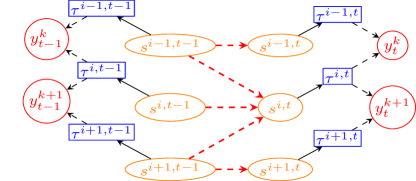
(a) Two time-slice bayesian net (2TBN) structure.

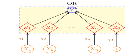
(b) NoisyOR: Proposed transition CPD model.

Figure 1: DBN structure and the proposed Transition CPD.

Conditional probability distributions on DBN

Observation CPD: Travel time distribution on a link $i$ given its state $s$, is assumed to be normally distributed with parameters $\mu^{i,s}$ and $\sigma^{i,s}$. We compactly refer to these observation parameters as ($\bm{\mu},\bm{\sigma}$). The travel time measurement from the $k^{th}$ vehicle at time epoch $t$, $y_{t,k}$ (denoted by circles in fig. 1(a)) is specified by the set of links traversed, $L_{t}(k)$, and position of the start and end co-ordinates on the first and last links (namely $x_{s,t}^{k}$ and $x_{e,t}^{k}$ respectively). $f(y^{k}_{t}|s^{L_{t}(k),t},x_{s,t}^{k},x_{e,t}^{k})$ denotes the conditional distribution of a travel-time measurement, conditioned on the links traversed and start-end positions. Given state information of links along a path, owing to normality and conditional independence of these travel times, travel time on any path is also normally distributed. The associated mean and variances are sum of mean and variances of individual link (possibly scaled) travel times.

Existing Transition CPDs: Let $A(\bm{\eta}^{i,t-1},s^{i,t})$ be the CPD that models influence exerted on road $i$’s state at time $t$ by $\bm{\eta}^{i,t-1}$, the states of its neighbors at time $t-1$. If this factor is a general tabular CPD as proposed in (?), then number of parameters grows exponentially with number of neighbors.

To circumvent this, (?) chooses a CPD whose number of parameters is linear in the number of neighbors. Instead of a separate bernoulli distribution for each realization of $\bm{\eta}^{i,t-1}$, it looks at the number of congested (or saturated) neighbors in the road network or parents in the DBN. Hence we refer to this as SatPat CPD in the rest of this paper. If $a_{i,j}$ denotes the chance of congestion at the $i^{th}$ link given exactly $j$ of its neighbors are congested at the previous time instant, then

$$A(\bm{\eta}^{i,t-1},s^{i,t})=\prod_{j=0}^{|\pi_{i}|}(a_{i,j})^{N^{i,t-1}_{j}s^{i,t}}(b_{i,j})^{N^{i,t-1}_{j}(1-s^{i,t})}$$ (1)

where $b_{i,j}=1-a_{i,j}$, and $N^{i,t-1}_{j}$ is an indicator random variable which is $1$ only when exactly $j$ of link $i$’s neighbors are congested. As mentioned earlier, this CPD has a few shortcomings:

• It assumes all neighbors of a road have identical influence on a road’s state. In particular it assumes an identical congestion probability (namely $a_{i,1}$) at $i$ at time $t$, given exactly one of its neighbors is congested at $t-1$. This is irrespective of which of $i$’s neighbors is congested at $t-1$.

• It is intuitive to expect that congestion probability of a road should increase with the number of congested neighbors, Specifically, one would expect that $a_{i,0}\leq a_{i,1}\leq\dots\leq a_{i,|\pi_{i}|}$. However, the learning strategy of (?) doesn’t ensure this total ordering. Hence, it may be difficult to interpret real world dependency among neighboring roads from learnt parameters.

Proposed Transition CPD: To alleviate the above short-comings, we propose to use a NoisyOR CPD (?) for modeling state transitions. If $Y\in\{0,1\},$ is the output and $\underline{X}=(X_{1},X_{2},\dots X_{n}),\>\>X_{k}\in\{0,1\},$ is the input, then the NoisyOR CPD is parameterized by $n+1$ parameters, viz. $(q_{0},q_{1},\dots q_{n}),0\leq q_{i}\leq 1$, referred to as inhibitor probabilities. The CPD is given by:

$$\vspace{-0.030in}P(Y=0|\underline{X})=q_{0}\prod_{k=0}^{n}q_{k}^{X_{k}},\>\>\>X_{k}\in\{0,1\}.$$ (2)

When $q_{0}=1$ and $q_{k}=0,\>\>\forall k>0$, we have the noiseless OR function. When one or more of the $q_{k}$s are non-zero, this CPD allows for a non-zero chance of the output becoming $0$ in spite of one or more high inputs. In our context, with $q_{0}$ clamped to $1$, each $q_{k}$ exactly captures the chance of output being $0$ (and hence the chance of congestion) when only the $k^{th}$ neighbor is congested. Hence, the NoisyOR (unlike SatPat) captures influence of neighboring links in an independent and link-dependent fashion – with $q_{k}$ representing the extent of influence from the $k^{th}$ neighbor. As the number of congested inputs (neighbors) go up, the chance of un-saturation goes down as is evident from eq. 2 . Hence it also captures the intuition of congestion probability increasing with the number of congested neighbors in the previous time step. $(1-q_{0})$ captures the chance of congestion getting triggered spontaneously at a link (while all its neighbors are uncongested).

Alternative representation for NoisyOR: The NoisyOR comes from the class of ICI (Independence of Causal Influence) models (?) and can be viewed as in Fig. 1(b) . On each input line $X_{k}$, there is a stochastic line failure function, whose output is $Z_{k}$. The deterministic OR acts on the $Z_{k}$s. When the input $X_{k}$ is zero, the line output $Z_{k}$ is also zero. When $X_{k}=1$, with inhibitor probability $q_{k}$, line failure happens – in other words, $Z_{k}$ is zero. The bias term $q_{0}$ controls the chance of the output being $1$ in spite of all inputs being off. It is easy to check that CPD in Fig. 1(b) is given by eq. 2 .

Under the NoisyOR CPD, the term which models the hidden state transitions can be expressed as $A({\bm{\eta}}^{i,t-1},\bar{\bm{\eta}}^{i,t-1},s^{i,t})$ where, ${\bm{\eta}}^{i,t-1}=\left[{\eta}^{i,t-1}_{1},{\eta}^{i,t-1}_{2},\dots,{\eta}^{i,t-1}_{|\pi_{i}|}\right]$ with ${\eta}^{i,t-1}_{j}$ representing the actual state of $i$’s neighbor $j$ at time $t-1$. Similarly, $\bar{\bm{\eta}}^{i,t-1}=\left[\bar{\eta}^{i,t-1}_{0},\bar{\eta}^{i,t-1}_{1},\dots\bar{\eta}^{i,t-1}_{|\pi_{i}|}\right]$ with $\bar{\eta}^{i,t-1}_{j}$ denoting the new random variable introduced via the representation of Fig. 1(b). Note that $\bar{\bm{\eta}}^{i,t}$ is of length $|(\pi_{i}+1)|$ while that of $\bm{\eta}^{i,t}$ is $|\pi_{i}|$. Based on Fig. 1(b), we can write $A({\bm{\eta}}^{i,t-1},\bar{\bm{\eta}}^{i,t-1},s^{i,t})$, the transition factor, as follows:

$$\begin{split}&A(\bm{\eta}^{i,t-1},\bm{\bar{\eta}}^{i,t-1},s^{i,t})\\ =&\,P(\bar{\eta}^{i,t-1}_{0})P(s^{i,t}|\bar{\bm{\eta}}^{i,t-1})\prod_{j=1}^{|\pi_{i}|}P(\bar{\eta}^{i,t-1}_{j}|\eta^{i,t-1}_{j})\\ =&\,q_{i,0}^{(1-\bar{\eta}^{i,t-1}_{0})}p_{i,0}^{\bar{\eta}^{i,t-1}_{0}}\mathds{1}_{\left\{\textrm{OR}(\bar{\bm{\eta}}^{i,t-1})=s^{i,t}\right\}}\\ &\,\prod_{j=1}^{|\pi_{i}|}(q_{i,j})^{\eta^{i,t-1}_{j}(1-\bar{\eta}^{i,t-1}_{j})}(p_{i,j})^{\eta^{i,t-1}_{j}\bar{\eta}^{i,t-1}_{j}}\end{split}$$ (3)

where $p_{i,j}=1-q_{i,j}$ and $q_{i,j}$ is the probability that congestion at time step $t-1$ in the $j^{th}$ neighbor of link $i$ does not influence $i$ in time step $t$. Similar to the SatPat CPD (eq.1), eq.3 demonstrates that a typical transition factor in the DBN under the NoisyOR CPD also belongs to the exponential family. This in turn makes M-step of EM learning feasible in closed form as explained later.

Complete data likelihood under NoisyOR: If $\mathbf{s}$ denotes the state of all links across all time, and $\mathbf{y}$ denotes the set of all travel time observations across all vehicles over time $t=1,\cdots,T$, the complete data likelihood is given by:

$$\vspace{-0.114in}\begin{split}p(\mathbf{s},\mathbf{y}|\bm{\theta})=&\prod_{\begin{subarray}{c}t=2\dots T\\ i\in\mathcal{I}\end{subarray}}A(\bm{\eta}^{i,t-1},\bar{\bm{\eta}}^{i,t-1},s^{i,t})\times\\ &\prod_{\begin{subarray}{c}t=1\dots T\\ k=1\dots N_{t}^{v}\end{subarray}}f(y_{t}^{k}|s^{L_{t}(k),t})\times\prod_{i\in\mathcal{I}}c^{i}(s^{i,1})\end{split}$$ (4)

where $c^{i}(0)$ is the marginal probability of link $i$ being uncongested at time $1$. We subsume this into $A(.,.,.)$ by constraining $c^{i}(0)=q_{i,0}$. This is same as assuming all links start at time $0$ uncongested. Note that, here $\bm{\theta}=(\bm{q},\bm{\mu},\bm{\sigma})$, where $\bm{q}$ refers to all NoisyOR parameters of each of the links.

4 Learning

An EM approach (App. C) is employed which is a standard iterative process involving two steps at each iteration. The E-step computes expectation of complete data log-likelihood ($Q$-function in short) at the current parameter values, while the $M$-step updates parameters by maximizing the $Q$-function. When the complete data log likelihood belongs to the exponential family, then learning gets simplified (?; ?). The $E$-step involves just computing the Expected Sufficient Statistics (ESS). The $M$-step typically consists of evaluating an algebraic expression based on the closed form maximum likelihood estimate (MLE) under completely observable data, in which SS is replaced by ESS.

E-step: E-step which involves ESS computation, is actually performing inference on a belief network. Exact inference in multiply connected belief networks is known to be NP-hard (?). Since our DBN is also multiply connected with a large number of links, exact inference would lead to unreasonable run times. Hence we use a sampling based approximation algorithm for inference (?). Specifically, we use a particle filtering approach. This involves storing and tracking a set of samples or particles. For each particle $r$, we start off with a vector of uncongested initial states for all the links. At each time step $t$, we grow each particle (sample) based on the current transition probability parameters(NoisyOR or SatPat). Each particle in state $s^{i,t}_{r}$ is now weighted by $\prod_{k=1\dots N_{t}^{v}}f(y_{t}^{k}|s^{L_{t}(k),t}_{r})$. An additional resampling of the particles based on these weights (normalized) is performed to avoid degeneracy. The required ESS (described above) are then estimated from these sample paths. As the name filtering indicates, the ESS at time $t$ is calculated based on observations up to time $t$, namely $\mathbf{y}^{t}$, rather than all observations. The ESS associated with observation parameters turns out to be $P(s^{L_{t}(k),t}=\bm{z}|\mathbf{y}^{t},\bm{\theta}^{\ell})\;\forall t,k,\bm{z}$. Here, $\bm{z}$ refers to a binary vector of length $|L_{t}(k)|$.

M-step Update for DBN model

Observation updates: From eq. 4 , it follows that $Q$-fn for the DBN model involves a sum of two terms: one exclusively a function of observation parameters ($\bm{\mu},\bm{\sigma}$) and the other only of the transition parameters ($\bm{q}$) for NoisyOR. Hence the joint maximization over ($\bm{\mu},\bm{\sigma}$) and ($\bm{q}$) gets decoupled. High time-resolution GPS observations are used to learn a 2-component Gaussian mixture at each link, which gives the means and variances of the individual link travel times. For convenient optimization, the variances thus obtained can be fixed and learning performed only over $\bm{\mu}$ as carried out in (?). However, one still needs iterative optimization owing to the complexity of the term involved.

Proposed transition parameters updates: Maximization of the second term involving hidden state transition parameters leads to an elegant closed-form estimate of the transition parameters for the proposed NoisyOR transitions. This is mainly because each factor belongs to the exponential family.

Proposition 1.

Given the observations $\mathbf{y}$ and parameter estimate after the $\ell^{th}$ EM-iteration, $\bm{\theta}^{\ell}$, the next set of transition parameters are obtained as follows.

$$\begin{split}q_{i,j}^{\ell+1}&\propto\sum_{t=2}^{T}P(\eta^{i,t-1}_{j}=1,\bar{\eta}^{i,t-1}_{j}=0|\mathbf{y},\bm{\theta}^{\ell})\\ p_{i,j}^{\ell+1}&\propto\sum_{t=2}^{T}P(\eta^{i,t-1}_{j}=1,\bar{\eta}^{i,t-1}_{j}=1|\mathbf{y},\bm{\theta}^{\ell})\end{split}$$ (5)

where proportionality constants are same. Similarly for $j=0$, the $M$-step updates are:

$$\begin{split}q_{i,0}^{\ell+1}&\propto\sum_{t=1}^{T}P(\bar{\eta}^{i,t-1}_{0}=0|\mathbf{y},\bm{\theta}^{\ell})\\ p_{i,0}^{\ell+1}&\propto\sum_{t=1}^{T}P(\bar{\eta}^{i,t-1}_{0}=1|\mathbf{y},\bm{\theta}^{\ell})\end{split}$$ (6)

Please refer to App. D for a proof. The proof involves computing the $Q$-function for the proposed NoisyOR CPD and maximizing it in closed form. The above ESS are actually computed conditioned on $\mathbf{y^{t}}$ (observations upto time t) and not $\mathbf{y}$, via particle filtering as explained in the E-step. Attempting smoothing which is exact, using all the observations $\mathbf{y}$, would lead to unreasonable space complexities, given the large number of links. The above updates are for data observations from a single day. They can readily be extended to multiple days and handled efficiently in a parallel fashion as explained in App. E . For a comparison of complexities between NoisyOR and SatPat, refer to App. F .

5 Prediction

Input: $\theta^{\star}$, Query Path $\Gamma=[i_{1},i_{2},\dots i_{|\Gamma|}]$, $\alpha_{s}$ - fractional distance of $x_{s}$ from downstream end of $i_{1}$.

Output: Mean Travel time (MTT) of traversing $\Gamma=[i_{1},i_{2},\dots i_{|\Gamma|}]$, starting at $t\Delta$ from $x_{s}$ on $i_{1}$.

1 Initialize $\textnormal{{MTT}}=0$, $\textnormal{{CurSuff}}=\Gamma$, $\textnormal{{CurSt}}=\alpha_{s}$, $\textnormal{{FutStep}}=1$, $\mathcal{P}=$ Set of particles grown upto $t$;

2 while $\textnormal{{CurSuff}}\neq\phi$ do

3       Grow all particles in $\mathcal{P}$ by one step (either as per NoisyOR or SatPat transitions);

4       $L:=\ell$-length prefix path of CurSuff, say $[i^{\prime}_{1},i^{\prime}_{2},\dots i^{\prime}_{\ell}]$. $\bm{b}_{k-1}$ := $\ell$-length binary representation of $(k-1)$.

5       $\bm{M}_{\ell}(k):=\textnormal{{CurSt}}*\mu^{i^{\prime}_{1},\bm{b}_{k-1}(1)}+\sum_{j=2}^{\ell}\mu^{i^{\prime}_{j},\bm{b}_{k-1}(j)}$, $\bm{p}_{\ell}(k):=P(s^{L,t+\textnormal{{FutStep}}}=\bm{b}_{k-1}|\mathbf{y^{t}},\theta^{\star})$, ($2^{\ell}$-length vectors).

6       if $\exists$ an $\ell$ s.t. $\bm{p}_{\ell}^{T}\bm{M}_{\ell}>\Delta$  then

7             Compute the least $\ell$ (say $c$) using binary search (Use $\mathcal{P}$, the current set of particles to compute $\bm{p}_{\ell}$) ;

8             if $c>1$ then

9                   $\textnormal{{CurSt}}\leftarrow 1-\{(\Delta-\bm{p}_{c}^{T}\bm{M}_{c}^{e-})/\bm{p}_{c}^{T}\bm{M}_{c}^{e}\}$, where $\bm{M}_{c}^{e-}$, $\bm{M}_{c}^{e}$ are $2^{c}$-length vectors;

10                   $\bm{M}_{c}^{e-}(k):=\textnormal{{CurSt}}*\mu^{i^{\prime}_{1},\bm{b}_{k-1}(1)}+\sum_{j=2}^{c-1}\mu^{i_{j},\bm{b}_{k-1}(j)}$, $\bm{M}_{c}^{e}=[\mu^{i_{c},0}\,\mu^{i_{c},1}\,\mu^{i_{c},0}\,\mu^{i_{c},1}\,\dots\mu^{i_{c},0}\,\mu^{i_{c},1}]^{T}$.

11                   $\textnormal{{CurSuff}}\leftarrow$ suffix of CurSuff (from $c$); $\textnormal{{MTT}}\leftarrow\textnormal{{MTT}}+\Delta$; $\textnormal{{FutStep}}\leftarrow\textnormal{{FutStep}}+1$;

12                  

13             end if

14            else  $\textnormal{{CurSt}}\leftarrow\textnormal{{CurSt}}(1-(\Delta/\bm{p}_{c}^{T}\bm{M}_{c}^{e}))$; $\textnormal{{MTT}}\leftarrow\textnormal{{MTT}}+\Delta$; $\textnormal{{FutStep}}\leftarrow\textnormal{{FutStep}}+1$ ;

15            

16       end if

17      else $\textnormal{{MTT}}\leftarrow\textnormal{{MTT}}+\bm{p}_{|\textnormal{{CurSuff}}|}^{T}\bm{M}_{|\textnormal{{CurSuff}}|}$; $\textnormal{{CurSuff}}=\phi$ ;

18      

19 end while

return MTT

Algorithm 1 Compute expected travel time of an aribitrary length query route

Formally, given $\bm{\theta}^{\star}$ (learnt DBN parameters from historical data) and current probe vehicle observations up to time $t\Delta$ (or time bin $t$), the objective is to predict the travel time of a vehicle that traverses a specified trajectory (or path) $\Gamma=[i_{1},i_{2},\dots i_{|\Gamma|}]$ starting at say $t\Delta$ (from time bin $(t+1)$). Existing works (?; ?) estimate the travel time along $\Gamma$ under the assumption that it is lesser than $\Delta$ (or one time step). However, in general, the travel times for a trajectory can be much more than $\Delta$.

Challenge: As the DBN evolves every $\Delta$ time units, the state of the DBN estimated at $(t+1)^{th}$ time bin can be used to predict the network travel times only in the associated time interval $[t\Delta,(t+1)\Delta)$. If the given trajectory $\Gamma$ is not fully traversed by $(t+1)\Delta$, the DBN’s state has to be advanced to time epoch $t+2$. The estimated network state at $t+2$ should now be used to predict the network travel time in the interval $[(t+1)\Delta,(t+2)\Delta)$, and so on. In other words, the task of predicting the travel time along $\Gamma=[i_{1},i_{2},\dots i_{|\Gamma|}]$ now gets transformed to the task of partitioning $\Gamma$ to contiguous trip segments $u_{1},u_{2},\dots,u_{M},$ such that the expected travel time of segment $u_{j},\>1\leq j\leq(M-1)$, is $\Delta$ time units as predicted using the hidden network state estimated at time epoch $(t+j)$; $u_{M}$ corresponds to the final trip segment in $\Gamma$ whose expected travel time is less than or equal to $\Delta$.

Approach: Without loss of generality, we assume that the end point $x_{e}$ of $\Gamma$ coincides with the end of link $i_{|\Gamma|}$. Algorithm 1 describes the procedure to predict the mean travel time, MTT, of $\Gamma$. App. G describes its correctness proof. CurSuff refers to the currently remaining suffix of $\Gamma$. CurSt is the fractional distance of the start point of CurSuff from the downstream intersection. $\bm{p}_{\ell}^{T}\bm{M}_{\ell}$ - Expected travel time of traversing a $\ell$-length prefix segment, $L=[i^{\prime}_{1},i^{\prime}_{2},\dots i^{\prime}_{\ell}]$, of CurSuff. The idea is to first narrow down on the earliest $\ell$ (say $c$) at which $\bm{p}_{\ell}^{T}\bm{M}_{\ell}>\Delta$. Subsequently, we need the exact position on $i^{\prime}_{c}$ upto which expected travel time is exactly $\Delta$. The main component of the proof explained in App. G involves how to arrive at this exact position via a closed-form. This is utilized in lines $9$ and $13$ of Algorithm 1. FutStep keeps track of additional number of time steps, particles are currently grown upto.

6 Experimental Results

(?), which propose the SatPat CPD clearly demonstrate how their approach outperforms baseline approaches based on time series ideas. Given this and comments made earlier in Sec. 2, we compare our proposed method with SatPat method only. We first test the efficacy of the methods on synthetic data. This is to better understand the maximum performance difference that can occur between the two approaches.

We implement learning by updating only the $\bm{q}$ (NoisyOR case) or $\bm{a}$ (SatPat case) parameters. During learning on synthetic data, we fix the observation parameters to the true values with which the data was generated. For ease of verification and since our contribution is in the M-update of hidden state transition parameters, we stick to this here. However, it is straightforward to include $\bm{\mu}$ as well in the iterative process as described in Sec. 4. The real data we consider in this paper is high time resolution probe vehicle data, where one can obtain independent samples of individual link times and learn a 2-component Gaussian mixture at each link. Another justification of our approach could be that there may not be a necessity to update $\bm{\mu}$ and $\bm{\sigma}$ once learnt via high time resolution GPS data.

We briefly summarize the synthetic data generation setup here and point the reader to App. I for additional details. The main idea is to use the DBN model of Sec. 3 with NoisyOR transitions and Gaussian travel times to generate trajectories. The generator takes as input a road network’s neighborhood structure and individual link lengths. The DBN structure is fixed from neighborhood information. The NoisyOR CPD gives a nice handle to embed a variety of congestion patterns. We choose CPD parameters to embed short-lived and long-lived congestions. The chosen synthetic network has $20$ links with gridded one-way roads mimicing a typical downtown area. We chose $8$ probe vehicles to circularly ply around the north-south region while another $8$ along the east-west corridor.

Results on synthetic traces

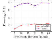
(a) Mean Absolute Error with increasing trip duration.

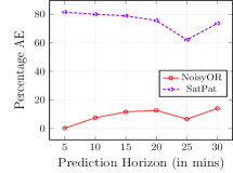
(b) Performance at maximum error difference.

Figure 2: Error vs prediction horizon (True Trip Duration) - long-lived congestions, $\Delta=5$ mins.

We compare prediction error between proposed and existing methods as (true) trip duration is gradually increased. Specifically, we use the clearly distinct NoisyOR learning scheme (proposed) and SatPat learning scheme (existing) for comparison (Sec. 4). For prediction however, we emphasize that the algorithm used for comparisons here (for both NoisyOR and SatPat schemes) is not an existing algorithm but rather a generic one proposed here in Sec. 5 which can tackle trips of arbitrary duration. We randomly pick from the testing trajectories of each of the $16$ probe vehicles, distinct non-overlapping trips of a fixed duration. We provide results of persisting (OR long-lived) congestion alone here. Results on short-lived congestion were found to be similar.

Each point in fig. 2(a) shows (Relative) Mean Absolute Error (MAE), obtained by averaging across all the distinct randomly chosen trips of a fixed duration (true trip time). ‘Relative’ here refers to error normalized by the true trip time. As true trip time (or prediction horizon) of the chosen trajectories is increased, the (MAE) also increases as intuitively expected. We also find that NoisyOR consistently gives more accurate predictions than SatPat justifying the need to model the varying influences of individual neighbors. For every prediction horizon, we also look for a trip on which difference in prediction errors between the proposed and existing approach is maximum. Fig. 2(b) gives the performance of both NoisyOR and SatPat with the maximum difference in prediction error, for a given prediction horizon. We see that prediction error difference can be as high as 70%, with NoisyOR being more accurate. Overall, it can be summarized that NoisyOR method’s predictions are significantly more accurate than the existing SatPat method. Further, NoisyOR learnt parameters can be interpreted better in real world than SatPat parameters.

Results on real-world probe vehicle data

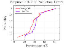
(a) Empirical CDF

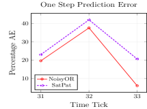
(b) Error time-series

Figure 3: City of Porto: Test trajectory duration=$\Delta$($5$ min).

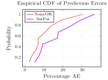
(a) Empirical CDF

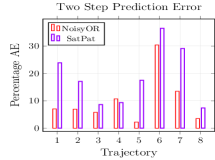
(b) Sample of Prediction Errors

Figure 4: San Francisco: Test trajectory duration = $2\Delta$($10$ min).

PORTO: To validate on real probe vehicle traces, we first used GPS logs of cabs operating in the city of Porto, Portugal. The data was originally released for the ECML/PKDD data challenge $2015$. Each trip entry consists of the start and end time, cab ID and a sequence of GPS co-ordinates sampled every $15$ seconds. The GPS co-ordinates in the data are noisy as many of them map to a point outside the road network. The GPS noise was removed using heuristics such as mapping a noisy point to one or more nearest links on the road network. The observation parameters $\mu^{i,s}$ and $\sigma^{i,s}$ are learnt for each link $i$ using the high resolution ($15$ sec) measurements as performed in (?). We fix observation parameters to these values and learn only the transition parameters.

We choose a connected region of the Porto map which was relatively abundant in car trajectories. This region consisted of roughly 100 links. App. J shows the actual region we narrowed down to. We chose a few second order neighbors (neighbor’s neighbor) too to better capture congestion propagation. Its very likely that a congestion originating at an upstream neighbor of a short link might actually propagate up to a down stream neighbor of the short link in question within $\Delta$ minutes. To account for this possibility, we add such second order neighbors (both upstream and downstream) to the list of original neighbors. We quantified short by links $<75$m in length and pick $\Delta=5$ min.

Trajectories from $4$ p.m. to $9$ p.m. were considered. One can expect the traffic conditions to be fairly stationary in this duration. The traffic patterns during a Friday evening can be very different from the other weekdays, which is why we treated Fridays separately. For sake of brevity, we discuss results obtained on Fridays alone. We trained on the best (in terms of the number of trajectories) $24$ Fridays. Training was carried out using both the proposed NoisyOR and existing SatPat CPDs. We tested the learnt parameters on two Fridays.

Fig. 3 shows the performance of both the proposed and SatPat method on trajectories (with true trip time equal to $\Delta$ minutes) one time epoch ahead of the current set of observations. Given the sparse nature of the data obtained, we focussed on testing trips of one $\Delta$ duration. Fig. 3(a) shows the empirical CDF of the absolute prediction errors (in $\%$). The empirical CDF essentially gives an estimate of the range of errors both the methods experienced. A relative left shift of the NoisyOR CPD prediction errors indicate a relatively better performance compared to SatPat. We also observe from the errors that the NoisyOR method has a relative absolute error of about $5\%$ lower than SatPat on an average and a relative absolute error of about $14.5\%$ lower in the worst case. Figure 3(b) gives a sequence of (one-step) prediction errors for both methods across a few consecutive time ticks around which data was relatively dense to report meaningful predictions. Note that the worst case error of $14.5\%$ was obtained at the $33^{rd}$ time tick around which NoisyOR method continues to do better than SatPat.

SAN FRANCISCO: We also considered a similar taxi data from a region (please refer to App. J for a map view) of the bay area of San Fransico. Specifically, we considered trajectories of $2\Delta$ duration for testing from this data. We trained both the NoisyOR and SatPat models on about $11$ days of data collected from this region of about $275$ links in the evening. We present results in Fig. 4 for test trajectories of $2\Delta$ duration. As before, the empirical CDF given in Fig. 4(a) has a relative left-shift in the NoisyOR’s CDF, indicative of its better performance. Further, Fig. 4(b) gives the trajectorywise prediction error comparison and an improvement of upto $16.8\%$ was observed in the worst case and about $6\%$ on an average.

This vindicates that the proposed technique of modeling influences of different roads in propagating traffic congestion can indeed be helpful. We also note that the worst case performance different between NoisyOR and SatPat is not as pronounced as in the synthetic traces. This could be attributed to the one of the following reasons: (i)the underlying congestion propagation characteristics may not be too much link dependent; (ii) even if the congestion propagation is link dependent, enough samples from probe vehicles may not be present in the available data logs.

7 Discussions and Conclusions

NoisyOR Based DBNs in Bioinformatics: We motivate one other concrete application where our NosiyOR based DBNs can be useful. Inferring gene regulation networks (?) from gene expression data is a very important problem in bioinformatics. Discovering the hidden excitatory/inhibitory interactions amongst the interacting genes is of interest here. DBN based approaches based on continuous hidden variables have been explored for this problem ((?)). The NoisyOR based DBN and the associated learning algorithm introduced in this paper can be a viable alternative to infer the underlying gene interactions by employing a fully connected structure among the interacting genes. The learnt $q_{i,j}$ values can potentially indicate the strength of influence. We intend exploring this further in our future work.

To conclude the paper, we proposed a balanced data driven approach to address the problem of travel time prediction in arterial roads using data from probe vehicles. We used a NoisyOR CPD in conjunction with a DBN to model the varying degrees of influence a given road may experience from its neighbors. We also proposed an efficient algorithm to learn model parameters. We also proposed an algorithm for predicting travel times of trips of arbitrary duration. Using synthetic data traces, we quantify the accuracy of the proposed method to predict the travel times of arbitrary duration trips under various traffic conditions. With the proposed approach, the prediction error reduces by as much as $50-70\%$ under certain conditions. We also tested the performance on traces of real data and found that the proposed approach fared better than the existing approaches. A possible future direction is to generalize the proposed approach to model road conditions using more than two states.

Appendix A Table of Symbols

Table 1: Notation used in this paper.

Symbol	Description
$\mathcal{I}$	Set of all links in the road network.
$\pi_{i}$	Set of links adjacent to road $i$, including itself.
$\Delta$	Size of a time bin or time between successive
	GPS measurements.
$s^{i,t}$	Random variable representing congestion state
	of road $i$ at time step $t$; $s^{i,t}\in\{0,1\}$.
$\mu^{i,s},\,\sigma^{i,s}$	Mean and std. deviation of the normally
	distributed travel time of link $i$ at state $s$.
$N^{v}_{t}$	Number of active vehicles at time step $t$.
$y_{t}^{k}$	travel time measurement at time step $t$ from the
	$k^{th}$ active vehicle; $k\in\{1,\dots,N_{t}^{v}\}$.
$L_{t}(k)$	Set of links traversed by the $k^{th}$ vehicle
	at time step $t$.
${x}_{s,t}^{k}$, ${x}_{e,t}^{k}$	Start and end locations of the $k^{th}$ active vehicle
	at time step $t$.
$\tau^{i,t}$	Actual travel time along link $i$ at time step $t$.
$A(.,.)$	Conditional distribution governing the link state
	transitions in the DBN.
$\bm{\eta}^{i,t}$	Vector of actual congestion states of
	$i$’s neighbors at $t$.
$\bar{\bm{\eta}}^{i,t}$	Vector representing influence exerted by $i$’s
	neighbors on $i$ at time $t$ under NoisyOR CPD.
$\bm{\theta}$	Complete parameter set governing the DBN.
$\bm{\theta}^{\star}$	Learnt parameters.
$q_{i,j}$	probability that congestion in the $j^{th}$ neighbor of
	$i$ at time step $t-1$ does not influence $i$ at time $t$.
$a_{i,j}$	congestion probability at the $i^{th}$ link given $j$ of its
	neighbors are congested at the previous instant.

Appendix B Summary of Travel Time Estimation Methods

Among the travel time estimation methods, a simple approach which uses a weighted average of real-time and historical data is proposed in (?). A more involved model which exploits the travel time correlation of nearby links to again perform travel time estimation using both historical and real-time travel data is proposed in (?). The work in (?) models link travel times by breaking them down to segments, assuming (dependent) gaussian travel times on each of these segments. Further a complex regression model which uses spatial correlation is used for network wide travel time estimation. A Markov chain approach for arterial travel time estimation was proposed recently in (?). An interesting approach based on tensor decomposition for city-wide travel time estimation based on GPS data has been proposed in (?). The current paper however deals with travel time prediction using probe vehicle data.

Appendix C EM algorithm

The EM algorithm is a popular method for learning on probabilistic models in the presence of hidden variables.The EM algorithm is fundamentally maximizing the observed data likelihood, namely $p(\mathbf{y}|\bm{\theta})$. Towards this, it employs an iterative process involving two steps (E-step and M-step) at each iteration.

Given the parameter estimate after the $\ell^{th}$ iteration, $\bm{\theta}^{\ell}$, the $E$-step computes the expected complete data loglikelihood defined as follows:

$$Q(\bm{\theta},\bm{\theta}^{\ell})=\sum_{s}p(\mathbf{s}|\mathbf{y},\bm{\theta}^{\ell})ln(p(\mathbf{y},\mathbf{s}|\bm{\theta}))$$ (7)

where the expectation is with respect to the conditional distribution $p(\mathbf{s}|\mathbf{y},\bm{\theta}^{\ell})$ computed at the current parameter estimate.

The $M$-step maximizes the above expected likelihood to obtain the next set of parameters, $\bm{\theta}^{\ell+1}$.

$$\bm{\theta}^{\ell+1}=\arg\!\max_{\bm{\theta}}Q(\bm{\theta},\bm{\theta}^{\ell})$$ (8)

The EM-algorithm increases the loglikelihood at each iteration and is guaranteed to converge to a local maximum of the data likelihood.

Appendix D Proof of Proposition 1

Proof.

NoisyOR CPD factor $A(.,.,.)$ appearing in eq. 4 can be expressed in terms of the associated bernoulli random variables and unknown link transition parameters $(\bm{q}^{i},\bm{p}^{i})$ as given in eq. 3. Taking log and expectation with respect to $p(\mathbf{s}|\mathbf{y},\bm{\theta}^{\ell})$ on both sides of eq. 3, we get the contribution of this factor in the Q-function (eq. 7 in App. C) as follows.

$$\begin{split}&log\left(E\left[A(\bm{\eta}^{i,t-1},\bm{\bar{\eta}}^{i,t-1},s^{i,t})\right]\right)\\ &=\sum_{j=1}^{|\pi_{i}|}E\left[\eta^{i,t-1}_{j}(1-\bar{\eta}^{i,t-1}_{j})\right]log(q_{i,j})+E\left[(\bar{\eta}^{i,t-1}_{0})\right]log(p_{i,0})\\ &+E\left[(1-\bar{\eta}^{i,t-1}_{0})\right]log(q_{i,0})+\sum_{j=1}^{|\pi_{i}|}E\left[\eta^{i,t-1}_{j}\bar{\eta}^{i,t-1}_{j}\right]log(p_{i,j})\end{split}$$

The various expectations can be simplified as:

$$E\left[\eta^{i,t-1}_{j}\bar{\eta}^{i,t-1}_{j}\right] = P(\eta^{i,t-1}_{j}=1,\bar{\eta}^{i,t-1}_{j}=1|\mathbf{y},\bm{\theta}^{\ell})$$

$$E\left[\eta^{i,t-1}_{j}(1-\bar{\eta}^{i,t-1}_{j})\right] = P(\eta^{i,t-1}_{j}=1,\bar{\eta}^{i,t-1}_{j}=0|\mathbf{y},\bm{\theta}^{\ell})$$

$$E\left[(1-\bar{\eta}^{i,t-1}_{0})\right] = P(\bar{\eta}^{i,t-1}_{0}=0|\mathbf{y},\bm{\theta}^{\ell})$$

$$E\left[(\bar{\eta}^{i,t-1}_{0})\right] = P(\bar{\eta}^{i,t-1}_{0}=0|\mathbf{y},\bm{\theta}^{\ell})\vspace{-0.11in}$$ (9)

For a fixed $i$ and $j$ ($j>0$), combining all terms involving $p_{i,j}$ and $q_{i,j}$ from the $Q$-fn, we obtain the following term.

$$\sum_{t=2}^{T}E\left[\eta^{i,t-1}_{j}(1-\bar{\eta}^{i,t-1}_{j})\right]log(q_{i,j})+E\left[\eta^{i,t-1}_{j}\bar{\eta}^{i,t-1}_{j}\right]log(p_{i,j})$$ (10)

where, $c_{i,j}=\sum_{t=2}^{T}E\left[\eta^{i,t-1}_{j}(1-\bar{\eta}^{i,t-1}_{j})\right]$, $d_{i,j}=\sum_{t=2}^{T}E\left[\eta^{i,t-1}_{j}\bar{\eta}^{i,t-1}_{j}\right]$ are the ESS associated with the transition parameters for the NoisyOR CPD.

To maximize the above expression (eq. 10) with respect to $q_{i,j}$ and $p_{i,j}$ with the constraint of $q_{i,j}+p_{i,j}=1$, the method of Lagrange multipliers yields the following Lagrangian

$$\mathscr{L}(q_{i,j},p_{i,j},\lambda)=c_{i,j}log(q_{i,j})+d_{i,j}log(p_{i,j})+\lambda(1-(q_{i,j}+p_{i,j}))$$ (11)

Differentiating the above equation and equating the first derivatives to zero, along with eq. D yields the (unnormalized) closed form solution as given in eq. 5. Similarly for $j=0$, a similar algebra yields eq. 6 . ∎

Appendix E Handling data from multiple days:

The updates in eq. 5 are for data observations from a single day. In general, we would learn from observations from multiple days under an i.i.d assumption between different days. In such a case, the right hand sides of the proportionality equations (eq. 5) will be involved in a double summation with the outer summation running over the day index similar to HMMs (?). The individual term calculation and inner summations can all be carried out in parallel i.e. for each day’s data before performing the outer summation across days to compute the next step transition parameters. Essentially, the $E$-step which computes ESS by using particle filtering can be carried out in parallel for each day. Hence the algorithm is amenable for parallelization and we exploit this aspect in our implementation.

Appendix F Complexity: SatPat vs NoisyOR

In comparison to eq. 5, the updates of the SatPat parameters (?) in the M-step would be as follows.

$$\begin{split}a_{i,j}^{\ell+1}\propto\sum_{t=1}^{T}P(\sum_{k=1}^{|\pi_{i}|}\eta^{i,t-1}_{k}=j,s^{i,t}=1|\mathbf{y},\theta^{\ell})\\ b_{i,j}^{\ell+1}\propto\sum_{t=1}^{T}P(\sum_{k=1}^{|\pi_{i}|}\eta^{i,t-1}_{k}=j,s^{i,t}=0|\mathbf{y},\theta^{\ell})\end{split}$$ (12)

For $j>0$, the first term in the above summation will be zero always as we start with all links in an uncongested state at time $0$.

While growing the particles there is a forward sampling step based on the transition probability structure. The introduction of the additional bernoulli random variables $\bar{\bm{\eta}}^{i,t-1}$ in the NoisyOR case at each link $i$, we would need to potentially sample once (a random number in $[0,1]$) for each of its neighbors. This means we would need to sample $(|\pi_{i}|+1)$ times in the worst case. For the same reason, one would also need to store an additional $|\pi_{i}|+1$ binary elements per link and per particle during NoisyOR learning. On the other hand for the SatPat CPD, one needs to compute the number of saturated neighbors (which is still an $\mathcal{O}(|\pi_{i}|)$ computation) but sample exactly once (irrespective of the no. of neighbors) to compute the congestion state of the link at the next time epoch. Since this is done for every particle, particle filtering run times are slightly higher for the NoisyOR CPD. Also while computing the ESS, in the E-step of the NoisyOR case, for each particle and each time bin (consecutive time bins), there is a contribution to potentially $|\pi_{i}|$ no. of ESS (in the worst case) associated with link $i$. As opposed to this, for the SatPat case, there is a contribution to exactly one ESS as is evident from the above equation.

Appendix G Correctness proof of Algorithm 1

Given a path $\Gamma=[i_{1},i_{2},\dots i_{|\Gamma|}]$, the conditional travel time distribution along $L$ at time $(t+1)$, given the current real time observations $\mathbf{y^{t}}$, is a mixture of Gaussians. The number of components in the mixture would be $2^{|\Gamma|}$, with each component weight being $P(s^{L,t+1}=\bm{b}|\mathbf{y^{t}},\theta^{\star})$, where $\bm{b}$ is a binary string of length $|\Gamma|$ that encodes the states of the individual links. Each associated component distribution of the mixture will itself be a sum of independent Gaussians with a mean of $\sum_{j=1}^{|\Gamma|}\mu^{i_{j},\bm{b}(j)}$. This follows from the conditional independence of the Gaussian travel times of links given the underlying state information (Section 3).

Consider a path $\Gamma=[i_{1},i_{2},\dots i_{|\Gamma|}]$ with a starting point $x_{s}$ on link $i_{1}$, with $\alpha_{s}$ the fractional distance of $x_{s}$ from the downstream intersection of $i_{1}$. For any prefix subpath of $\Gamma$ of length $\ell$ ($L=[i_{1},i_{2},\dots i_{\ell}]$, $\ell\leq|\Gamma|$), we introduce two $2^{\ell}$-length vectors $\bm{M}_{\ell}$ and $\bm{p}_{\ell}$. $\bm{M}_{\ell}$ denotes the mean vector of all the components of the Gaussian mixture distribution modeling the travel time across $L$. Specifically, $\bm{M}_{\ell}(k)=\alpha_{s}\mu^{i_{1},\bm{b}_{k-1}(1)}+\sum_{j=2}^{\ell}\mu^{i_{j},\bm{b}_{k-1}(j)}$, where $\bm{b}_{k}$ is the $\ell$-length binary representation of integer $k$. We further assume $\bm{b}_{k}(1)$ is the MSB, while $\bm{b}_{k}(\ell)$ is the LSB of this binary representation. Similarly, $\bm{p}_{\ell}$ is the vector of mixture weights of this gaussian mixture, where $\bm{p}_{\ell}(k)=P(s^{L,t+1}=\bm{b}_{k-1}|\mathbf{y^{t}},\theta^{\star})$.

Reweighted particles already spawned till time $t$ are now grown by one step to compute each of the components of $\bm{p}_{\ell}$ (line $3$ of Algorithm 1). In general, all particles currently at $(t+\textnormal{{FutStep}}-1)$ are grown by one step as per the state transition structure (NoisyOR or SatPat).

The mean travel time across any expanding path $L$ will be $\bm{p}_{\ell}^{T}\bm{M}_{\ell}$. We look for the least $\ell$ such that $\bm{p}_{\ell}^{T}\bm{M}_{\ell}>\Delta$ (line $6$ of Algorithm 1). Let $c$ be the least $\ell$ satisfying this. The mean travel time along an expanding prefix path $L$ is an increasing function of $\ell$. Hence to compute $c$, binary search would be more efficient (line $7$ of Algorithm 1). In other words, we find the first link $i_{c}$ along the trajectory $\Gamma$ where the mean travel time from $x_{s}$ becomes greater than $\Delta$. After finding $i_{c}$, we find the precise location $x_{c}$ on the link $i_{c}$ such that the mean travel time from $x_{s}$ to this point equals $\Delta$. This point $x_{c}$ can be determined using a closed form expression as shown below (line $9$ or line $13$ of Algorithm 1).

Let $\alpha_{c}$ denote the fractional distance of $x_{c}$ from the upstream intersection of $i_{c}$. Consider a $2^{c}$-length vector $\bm{M}_{c}^{\alpha}$ ($0\leq\alpha\leq 1$), where

$$\begin{split}\bm{M}_{c}^{\alpha}(k)=\alpha_{s}\mu^{i_{1},\bm{b}_{k-1}(1)}+\sum_{j=2}^{c-1}\mu^{i_{j},\bm{b}_{k-1}(j)}+\alpha\mu^{i_{c},\bm{b}_{k-1}(c)},\\ k=1,2,\dots,2^{c}.\end{split}$$ (13)

In the above equation, note that $\bm{b}_{k-1}$ is a $c$-length binary representation of $(k-1)$. To obtain $\alpha_{c}$, we solve for $\alpha$ in the equation $\bm{p}_{c}^{T}\bm{M}_{c}^{\alpha}=\Delta$. Towards solving this, we first recognize from eq.(13) that $\bm{M}_{c}^{\alpha}=(\bm{M}_{c}^{e-}+\alpha\bm{M}_{c}^{e})$, essentially a sum of two other $2^{c}$-length vectors, one independent and the other dependent on $\alpha$. Here, each component of $\bm{M}_{c}^{e-}$ can be written as ( definition on line $10$ of Algorithm 1 )

$$\bm{M}_{c}^{e-}(k)=\alpha_{s}\mu^{i_{1},\bm{b}_{k-1}(1)}+\sum_{j=2}^{c-1}\mu^{i_{j},\bm{b}_{k-1}(j)}$$ (14)

Further, by our convention, $\bm{b}_{k-1}(c)$ is the LSB of the binary representation of $(k-1)$. Hence we have $\bm{M}_{c}^{e}=[\mu^{i_{c},0}\,\mu^{i_{c},1}\,\mu^{i_{c},0}\,\mu^{i_{c},1}\,\dots\mu^{i_{c},1}]^{T}$, which is equivalent to $\bm{M}_{c}^{e}(k):=\mu^{i_{c},(k-1)\pmod{2}}$ ( definition on line $10$ of Algorithm 1 ). Now substituting for $\bm{M}_{c}^{\alpha}$ by $(\bm{M}_{c}^{e-}+\alpha\bm{M}_{c}^{e})$ and a term rearrangement yields

$$\begin{split}\alpha_{c}&=(\Delta-\bm{p}_{c}^{T}\bm{M}_{c}^{e-})/\bm{p}_{c}^{T}\bm{M}_{c}^{e}\end{split}$$ (15)

$\alpha_{c}$ denotes the fractional distance of $x_{c}$ from the upstream end. Since CurSt captures the fractional distance from the downstream end, we set CurSt to $1-\alpha_{c}$ as per line $9$ of Algorithm 1 ). CurSuff is now set to the suffix of the previous CurSuff ($\Gamma$ in the first iteration) that starts from the $c^{th}$ position. Mean Travel Time MTT is incremented by $\Delta$ as a segment with mean travel time $\Delta$ is consumed (line $11$).

On the other hand if $c=1$, $\bm{p}_{1}^{T}\bm{M}_{1}^{e}>\Delta$. $\bm{p}_{1}^{T}\bm{M}_{1}^{e}$ is the time taken to travel the rest of $i^{\prime}_{1}$ OR a fractional distance CurSt. Therefore in a time of $\Delta$, the fractional distance travelled is $(\textnormal{{CurSt}}*\Delta/\bm{p}_{c}^{T}\bm{M}_{c}^{e})$ to obtain $x_{c}$. The fractional distance of $x_{c}$ from the downstream end of $i^{\prime}_{1}$ would be $\textnormal{{CurSt}}-(\textnormal{{CurSt}}*\Delta/\bm{p}_{c}^{T}\bm{M}_{c}^{e})$ (line $13$ of Algorithm 1 ).

If the current suffix CurSuff is such that $\nexists$ an $\ell$ satisfying $\bm{p}_{\ell}^{T}\bm{M}_{\ell}>\Delta$, then this means we have hit the last segment and MTT is accordingly incremented by the mean travel time of CurSuff, the last segment (line $15$ of Algorithm 1).

Appendix H Correctness of implementation

Any EM algorithm necessarily increases the likelihood of the data at every iteration. In order to verify this necessary condition, we additionally implemented a routine to calculate the likelihood of the data given a current set of transition and observation parameters. The implementation is based on the forward-backward algorithm for inference in HMMs(?). In the current case, if all the link states at a fixed time are stacked together as a vector, then the sequence of joint vectors of hidden link states exactly forms a markov chain. We would need the transition probability matrix which can be calculated based on the transition CPD used. Note the observations at each time epoch are not the link travel times directly but a certain linear combination of one more link travel times depending on the vehicle trajectory. In addition to the transition probability matrix one needs to compute the probability of having traversed each of these trajectories in a time of $\Delta$ units, given the underlying state vector. This is readily computable as the travel times given the underlying states are independent gaussians, which means the distribution of their appropriate sums are also gaussian. Since the no. of states of this markov chain grows exponentially with the number of links, the transition matrix and likelihood computation do not scale with no. of links. However, for tiny networks one can use this to compute likelihoods and hence verify the correctness of implementation.

On running learning algorithms (NoisyOR and SatPat) on a 3-link network to learn the transition parameters alone with fixed means and variances (to the true values), results were as expected. We observed the log likelihoods of the parameter iterates to always increase and generally converge to the true parameter loglikelihoods.

Appendix I Synthetic Data

Testing the algorithms on synthetic data has the following advantages: (a) since the ground truth information is available in a synthetic setup, we can precisely validate the goodness of learning. (b) it also gives us a handle to compare performance of the proposed and existing approaches under different congestion patterns.

Trace Generation Setup

The synthetic data generator is fed with a road network containing a certain number of links along with their lengths and a neighborhood structure. Based on this neighborhood structure, we feed the generator a transition probability structure that governs the congestion state transitions of the individual links from time $t$ to time $t+1$. The conditional travel times for each link $i$ and state $s$, is assumed to be normally distributed with appropriate parameters $\mu^{i,s}$ and $\sigma^{i,s}$ as described earlier in Sec. 3 . $\mu^{i,0}$ and $\mu^{i,1}$ capture the average travel times experienced by commuters during congestion and non-congestion due to intersections or traffic lights. The $\sigma$ parameter captures the continuum of congestion levels actually possible. The link states are assumed to make transitions at a time scale approximately equal to $\Delta$.

Data Generation: One or more probe vehicles traverse a subset of links in a predetermined order repeatedly. The paths and vehicles are so chosen that there is sufficient coverage of all the links across space and time. The link states are stochastically sampled with time as per the prefixed transition probability structure. Given the state of all the links at a particular time epoch, we now describe how the trajectories are generated for the probe vehicles. Let us say a vehicle is at a position $x_{s}$ at the start of a time epoch of $\Delta$ units. The idea is to exhaust these $\Delta$ units along the (prefixed) path of the vehicle and arrive at the appropriate end position $x_{e}$. Suppose $x_{s}$ is at a link $i$ and at a distance of $d_{e}$ from the end of link $i$. Given that link $i$ is in state $s$, we sample once from $\mathcal{N}(y;\mu^{i,s},\sigma^{i,s})$ to obtain a realization of $\tau^{i,t}$. Let $y$ be the sampled value which corresponds to the time to travel from the start to the end of link $i$ in the current epoch. By linear scaling the time taken to traverse a distance of $d_{e}$ would be $y\frac{d_{e}}{len(i)}$. If this time is greater than $\Delta$, then the vehicle doesn’t cross link $i$ in the current time epoch and settles into a position $x_{e}$ which is $len(i)\frac{\Delta}{y}$ units further from $x_{s}$. However if the time to traverse the rest of the link, namely $(yd_{e})/len(i)$, is less than $\Delta$, then the vehicle is moved to the start of the next link in its prefixed path. Further, now a residual time of $\Delta-yd_{e}/len(i)$ needs to exhausted along the subsequent path and the process described is continued till the residual time is completely exhausted to reach a final position $x_{e}$. This process of trajectory formation is carried out for each vehicle at each discrete time epoch.

Figure 5: Synthetic topology of 20 links

Network Structure: The network structure chosen consists of 20 links as shown in figure 5. We chose this structure since it represents the gridded one-way roads that are typically found in the downtown area of various cities. It consists of a long sequence of unidirectional lanes in either direction connecting point $A$ (in the north) to a point $B$ (in the south). Traffic moving from $A$ to $B$ (north to south) have to go along links $1$ to $5$, while travelers need to take links $6$ to $10$ for their return. Similarly there is a road infrastructure that connects $C$ (in the east) to $D$ (in the west) via links $11$ to $20$. This synthetic topology has a relatively rich neighbourhood structure with peripheral links like $1$, $6$, $11$, $16$ having $3$ neighbors (including themselves) while links $3$, $13$, $8$ and $18$ at the center having up to $5$ neighbors (including themselves). All links are assumed to have the same length of $1$ km. For each link $i$, $\mu^{i,0}=1.5$ min, $\mu^{i,1}=3.0$ min, $(\sigma^{i,0})=(\sigma^{i,1})=0.1$. With $\Delta$ fixed at $5$ minutes, we chose about $60$ time steps for data generation and generated such sequences for $8$ days ($8$ i.i.d. realizations). We choose to use $8$ probe vehicles which move along the north-south circular loop between A and B. Similarly, we also have another set of 8 probe vehicles moving east-west between C and D.

Congestion Patterns: We embed a short-lived congestion which can randomly originate at either link $1$, $6$, $11$ or $16$. Once congestion starts at a link, say link $1$, it moves downstream to link $2$ with probability $1$ at the next time step and this process continues unidirectionally till link $5$. A similar congestion pattern which moves downstream one link at a time at every subsequent time step is embedded starting from link $6$, $11$ and $16$. Congestion doesn’t persist in the same link into the next time step in any of the links – these are short-lived congestions. Such short-lived congestion happens in real-world when a wave of vehicles traverse the links.

The above described short-lived congestion can be modeled using a NoisyOR based data generator. The random chance of congestion originating at link $1$ can be captured by setting $p_{1,0}$ to a low value, say $0.2$. The rest of the neighbors of $1$, (namely $1$, $2$ and $10$) do not influence $1$ and hence the respective $p_{1,j}$s will all be zero. At link $2$, to embed the $1^{st}$ link’s strong influence, we set $p_{2,1}=1$. Since there is no congestion persistence, we set $p_{2,2}=0$. Since we assume there is no upstream influence of congestion, we set $p_{2,3}=0$. Similarly, the parameters for other links are chosen.

We also generate data with non-zero probabilities for congestion to persist for longer duration in a link. This means for a link $i$, $p_{i,j}$ (where $j$ refers to the self-neighbor) must be set to a non-zero value. We have chosen this value to be around $0.1$ across all links. This non-zero chance ensures some of the links once congested will continue to remain congested for one or more subsequent time steps.

Appendix J Map of the considered regions

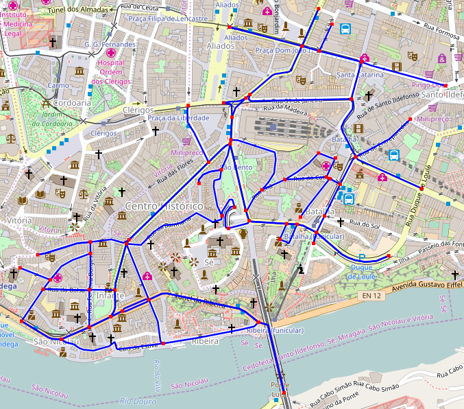
Figure 6: Region of Porto on which Cab traces were considered.

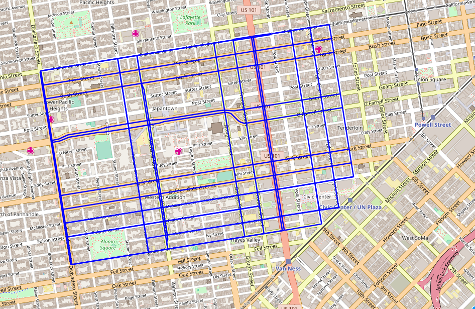
Figure 7: Region of SanFransisco on which Cab traces were considered.

References

- [Aslam et al. 2012] Aslam, J.; Lim, S.; Pan, X.; and Rus, D. 2012. City-scale traffic estimation from a roving sensor network. In Proceedings of the 10th ACM Conference on Embedded Network Sensor Systems, SenSys ’12, 141–154. New York, NY, USA: ACM.
- [Bishop 2006] Bishop, C. M. 2006. Pattern Recognition and Machine Learning (Information Science and Statistics). Secaucus, NJ, USA: Springer-Verlag New York, Inc.
- [Cooper 1990] Cooper, G. F. 1990. The computational complexity of probabilistic inference using bayesian belief networks. Artificial Intelligence 42(2-3):393–405.
- [El Esawey and Sayed 2010] El Esawey, M., and Sayed, T. 2010. Travel time estimation in urban networks using buses as probes. In Annual conference of the Transportation Association of Canada, Halifax, Nova Scotia, 1–22.
- [Heckerman and Breese 1994] Heckerman, D., and Breese, J. S. 1994. A new look at causal independence. In Proceedings of the Tenth International Conference on Uncertainty in Artificial Intelligence, UAI’94, 286–292.
- [Herring et al. 2010] Herring, R.; Hofleitner, A.; Abbeel, P.; and Bayen, A. 2010. Estimating arterial traffic conditions using sparse probe data. In 13th Int. IEEE Conf. on Intelligent Transportation Systems, 929–936.
- [Hofleitner et al. 2012] Hofleitner, A.; Herring, R.; Abbeel, P.; and Bayen, A. 2012. Learning the dynamics of arterial traffic from probe data using a dynamic bayesian network. IEEE Transactions on Intelligent Transportation Systems 13(4):1679–1693.
- [Hofleitner, Herring, and Bayen 2012] Hofleitner, A.; Herring, R.; and Bayen, A. 2012. Arterial travel time forecast with streaming data: A hybrid approach of flow modeling and machine learning. Transportation Research Part B: Methodological 46(9):1097–1122.
- [Hofleitner 2013] Hofleitner, A. 2013. A hybrid approach of physical laws and data-driven modeling for estimation: the example of queuing networks. Ph.D. Dissertation, EECS Department, University of California, Berkeley.
- [Hunter et al. 2009] Hunter, T.; Abbeel, P.; Herring, R.; and Bayen, A. 2009. Path and travel time inference from gps probe vehicle data. In In NIPS Analyzing Networks and Learning with Graphs.
- [Hunter et al. 2011] Hunter, T.; Moldovan, T.; Zaharia, M.; Merzgui, S.; Ma, J.; Franklin, M. J.; Abbeel, P.; and Bayen, A. M. 2011. Scaling the mobile millennium system in the cloud. In Proceedings of the 2nd ACM Symposium on Cloud Computing, SOCC ’11, 28:1–28:8. New York, NY, USA: ACM.
- [Ishak and Al-Deek 2003] Ishak, S., and Al-Deek, H. 2003. Statistical evaluation of interstate 4 traffic prediction system. Transportation Research Record: Journal of the Transportation Research Board (1856):16–24.
- [Jenelius and Koutsopoulos 2013] Jenelius, E., and Koutsopoulos, H. N. 2013. Travel time estimation for urban road networks using low frequency probe vehicle data. Transportation Research Part B: Methodological 53:64–81.
- [Karlebach and Shamir 2008] Karlebach, G., and Shamir, R. 2008. Modelling and analysis of gene regulatory networks. Nat Rev Mol Cell Biol 9:770–780.
- [Koller and Friedman 2009] Koller, D., and Friedman, N. 2009. Probabilistic Graphical Models: Principles and Techniques - Adaptive Computation and Machine Learning. The MIT Press.
- [Kwon, Coifman, and Bickel 2000] Kwon, J.; Coifman, B.; and Bickel, P. 2000. Day-to-day travel-time trends and travel-time prediction from loop-detector data. Transportation Research Record: Journal of the Transportation Research Board (1717):120–129.
- [Li and Rose 2011] Li, R., and Rose, G. 2011. Incorporating uncertainty into short-term travel time predictions. Transportation Research Part C: Emerging Technologies 19(6):1006–1018.
- [Liu, Yue, and Krishnan 2013] Liu, S.; Yue, Y.; and Krishnan, R. 2013. Adaptive collective routing using gaussian process dynamic congestion models. In Proceedings of the 19th ACM SIGKDD International Conference on Knowledge Discovery and Data Mining, KDD ’13, 704–712. New York, NY, USA: ACM.
- [Mori et al. 2015] Mori, U.; Mendiburu, A.; Álvarez, M.; and Lozano, J. A. 2015. A review of travel time estimation and forecasting for Advanced Traveller Information Systems. Transportmetrica A: Transport Science 11(2):119–157.
- [Nikovski et al. 2005] Nikovski, D.; Nishiuma, N.; Goto, Y.; and Kumazawa, H. 2005. Univariate short-term prediction of road travel times. In Proceedings. 2005 IEEE Intelligent Transportation Systems, 2005., 1074–1079. IEEE.
- [Perrin et al. 2003] Perrin, B.-E.; Ralaivola, L.; Mazurie, A.; Bottani, S.; Mallet, J.; and d’Alché–Buc, F. 2003. Gene networks inference using dynamic bayesian networks. Bioinformatics 19(suppl_2):ii138–ii148.
- [Pu, Lin, and Long 2009] Pu, W.; Lin, J.; and Long, L. 2009. Real-time estimation of urban street segment travel time using buses as speed probes. Transportation Research Record: Journal of the Transportation Research Board 2129:81–89.
- [Ramezani and Geroliminis 2012] Ramezani, M., and Geroliminis, N. 2012. On the estimation of arterial route travel time distribution with markov chains. Transportation Research Part B: Methodological 46(10):1576–1590.
- [Vanajakshi, Subramanian, and Sivanandan 2009] Vanajakshi, L.; Subramanian, S.; and Sivanandan, R. 2009. Travel time prediction under heterogeneous traffic conditions using global positioning system data from buses. IET intelligent transport systems 3(1):1–9.
- [Wang, Zheng, and Xue 2014] Wang, Y.; Zheng, Y.; and Xue, Y. 2014. Travel time estimation of a path using sparse trajectories. In Proceedings of the 20th ACM SIGKDD International Conference on Knowledge Discovery and Data Mining, KDD ’14, 25–34. ACM.