Learning and Visualizing Localized Geometric Features Using 3D-CNN: An Application to Manufacturability Analysis of Drilled Holes

Abstract

3D Convolutional Neural Networks (3D-CNN) have been used for object recognition based on the voxelized shape of an object. However, interpreting the decision making process of these 3D-CNNs is still an infeasible task. In this paper, we present a unique 3D-CNN based Gradient-weighted Class Activation Mapping method (3D-GradCAM) for visual explanations of the distinct local geometric features of interest within an object. To enable efficient learning of 3D geometries, we augment the voxel data with surface normals of the object boundary. We then train a 3D-CNN with this augmented data and identify the local features critical for decision-making using 3D GradCAM. An application of this feature identification framework is to recognize difficult-to-manufacture drilled hole features in a complex CAD geometry. The framework can be extended to identify difficult-to-manufacture features at multiple spatial scales leading to a real-time design for manufacturability decision support system.

1 Introduction

Deep learning (DL) algorithms, more specifically 3D-Convolutional Neural Networks (3D-CNN), hierarchically learn multiple levels of abstractions of the data. They have been extensively used in computer vision (Sarkar et al., 2015; Lee et al., 2009; Lore et al., 2016; Larochelle and Bengio, 2008), specifically for object recognition. However, learning local features in a geometry is different from object recognition where the object is classified based on a collection of features. In this work, we make use of a semi-supervised methodology to learn localized geometric features of interest within the object based on the cost function of the overall object classification problem. For this purpose, we train a 3D-CNN to learn the key features of the object and also learn the variation in the features that can classify the object based on a given cost function. We make use of a voxelized 3D representation of the object augmented with surface normal information to identify these localized features.

One applications of the aforementioned methodology, which we explore in this paper, is to identify difficult-to-manufacture features in a CAD geometry and ultimately, classify its manufacturability. There are different handcrafted design for manufacturability (DFM) rules that ensure manufacturability of a design. For this purpose, the hierarchical architecture of DL can be used to learn increasingly complex features by capturing localized geometric features and feature-of-features. Thus, a deep-learning-based design for manufacturing (DLDFM) tool can be used to learn the various DFM rules from different examples of manufacturable and non-manufacturable components without explicit handcrafting.

A primary concern while examining the manufacturability of CAD geometries using a DL based approach is the black-box nature of such deep networks. Interpretation of the decision making process in the form of visual explanations is essential for extracting the local features in an object that effects its non-manufacturability. Visual detection of local features further enables re-designing of the component or object to abide the various DFM rules. Recent major work on interpreting DL output by Selvaraju et al. (2016) makes use of a 2D gradient-weighted class activation map for producing visual explanations of the CNN’s decision making processes in object recognition in images. In this work, we extend the GradCAM to 3D objects for interpretation of 3D-CNN’s outputs and visualizing the regions that give rise to non-manufacturability conditions in the objects.

In this paper, we present a 3D convolutional neural network (3D-CNN) based framework that will learn and identify localized geometric features from an expert database in a semi-supervised manner. Further, we present a visual explanation technique using GradCAM to interpret the decision making process in the context of manufacturability with different CAD models classified as manufacturable and non-manufacturable.

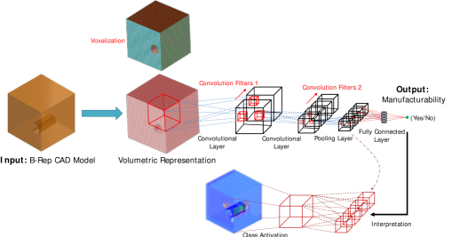
Figure 1: Framework for deep-learning based design for manufacturability. The CAD model is converted to a voxel representation and is input to a 3D-CNN for manufacturability classification. The 3D-CNN output is analyzed using 3D-gradCAM to provide manufacturability feedback.

2 Volumetric Representations for Learning Geometric Features

Traditional CAD systems use boundary representations (B-Reps) to define and represent the CAD model Krishnamurthy et al. (2009). In B-Reps, the geometry is defined using a set of faces that form the boundary of the solid object. B-Reps are ideally suited for displaying the CAD model by first tessellating the surfaces into triangles and using the GPU to render them. In our framework, we convert the B-Rep CAD model to a volumetric occupancy grid of voxels using a rendering-based approach. For representing a 3D object with more information regarding its geometry, we augment the boundary voxels with the surface normals of the B-Rep geometry. Finally,the $x,y,$ & $z$ components of the surface normals are then embedded in the voxelization along with the occupancy grid to be used as four-channel input to the 3D-CNN.

3 3D-CNN for Learning Localized Geometric Features

The input to the 3D-CNN is a zero-padded voxelized CAD model. The convolution layer is activated with RELU function and is followed by batch normalization layer and a max. pooling layer. The same sequence of convolution, batch normalization and max. pooling is used again. A fully connected layer is used before the final output layer (manufacturability) with sigmoid activation. The model parameters $\theta$, comprised of weights W, and biases, b are optimized by error back-propagation with binary cross-entropy loss function (Hinton and Salakhutdinov, 2006) using the ADADELTA optimizer (Zeiler, 2012).

Several different CAD models were generated based on the DFM rules for drilling using ACIS (Spatial Corporation, 2009), a commercial CAD modeling kernel, for training the network. DFM rules for drilled holes are based on inter-related local geometric features such as the depth-to-diameter ratio (Boothroyd et al., 2002; Bralla, 1999) and the presence of thin walls surrounding the hole. These rules were used to classify the models as manufacturable or non-manufacturable.

4 Interpretation of 3D-CNN Output

The trained 3D-CNN network can be used to classify the manufacturability of any new geometry and can be treated as a black box. In a practical scenario, interpretability and explainability of the output provided by the 3D-CNN is essential. In this paper, we attempt to visualize the input features that lead to a particular output of the 3D-CNN and if possible, modify it. A similar approach was used in object recognition in images by using class activation maps to obtain class specific feature maps by Selvaraju et al. (2016). The class specific feature maps could be obtained by taking a class discriminative gradient of the prediction with respect to the feature map for the class activation. In this paper, we present the first application of 3D gradient weighted class activation map (3D-GradCAM) for recognizing local features in a 3D object.

In order to get the feature localization map using 3D-GradCAM, we need to compute the spatial importance of each feature map $A_{l}$ in the last convolutional layer of the 3D-CNN, for a particular class, $c$ ($c$ can either be manufacturability or non-manufacturability, for the sake of generality) in the classification problem. This spatial importance for each feature map can be interpreted as weights for each feature map; it can be computed as the global average pooling of the gradients back from the specific class of interest as shown in Eqn. 2.

The cumulative spatial importance activations that contribute to the class discriminative localization map, $L_{3DGradCAM}$, is computed using

$$L_{3DGradCAM}=ReLU\left(\sum_{l}{\alpha_{l}\times A^{l}}\right),$$ (1)

where $\alpha_{l}$ are the weights computed using

$$\alpha_{l}=\frac{1}{Z}\times\sum_{i}{\sum_{j}{\sum_{k}{\frac{\partial y^{c}}{\partial A_{ijk}^{l}}}}}.$$ (2)

We can compute the activations obtained for the input using $L_{3DGradCAM}$ to analyze the source of output. The heat map of $\left(L_{3DGradCAM}\right)$ is resampled using linear interpolation to match the input size, and then overlaid in 3D with the input to be able to spatially identify the source of non-manufacturability. This composite data is finally rendered using a volume renderer.

We make use of a GPU-based ray-marching approach to render this volume data. The rendering is parallelized on the GPU with each ray corresponding to the screen pixel being cast independently. The intersection of the ray with the bounding-cube of the voxel data is computed, and then the 3D volumetric data is sampled at periodic intervals. The sum of all the sampled values along the ray is then computed. This value is converted to RGB using a suitable color scale and rendered on the screen. Table 2 shows different volumetric renderings of the composite 3D-GradCAM data.

5 Results and Discussion

Table 1: Quantitative performance assessment of the DLDFM on test data sets.

=.1in =2.5in Test Data Type Model Description True Positive True Negative False Positive False Negative Accuracy 675 models 408 Manufacturable In-outs 391 90 17 176 0.7136 In-outs + Surface Normals 334 201 74 65 0.7938

The generated CAD geometries are classified to be manufacturable or non-manufacturable based on the DFM rules for drilled holes. The 3D-CNN (explained in Section 3) is trained on the generated data with fine-tuned hyper-parameters to have the least validation loss. The architecture of the DLDFM network with voxelized information is composed of three convolution layers with filter sizes of 8, 4, and 2 respectively. Likewise, the DLDFM networks using surface normal along with voxelized representation, comprises of three convolution layers with filter sizes of 6, 3, and 2 respectively. In succession to the first and last Convolution layers, we use MaxPooling layers of subsampling size 2. A batch size of 64 is selected while training the DLDFM networks. The training was performed using Keras (Chollet, 2015) with a TensorFlow (Abadi et al., 2015) backend in Python environment. The training is performed until the validation loss remains constant for at least 10 consecutive epochs.

After successful training, the DLDFM network was tested on a test set to benchmark its performance. Accuracy of DLDFM network on the test set using the two data representations is shown in Table 1. The test-set has completely different geometries compared to the training set. Thus, it can be seen that the DLDFM is learning the localized geometric features.

Table 2: Illustrative examples of manufacturability prediction and interpretation using the DLDFM framework.

=.1in =2.5in CAD Models Manufacturable Non-Manufacturable Non-Manufacturable Non-Manufacturable 3D-GradCam Visualizations

Using the trained DLDFM network, it is possible to obtain the localization of the feature activating the decision of the DLDFM. The 3D-GradCAM renderings for various cases are shown in the Table 2. We have used 3D-GradCAM to visualize the results of various inputs such as manufacturable holes, non-manufacturable-holes, multiple holes in same face, and holes in multiple faces of the cube. 3D-GradCAM can localize the features that can cause the part to be non-manufacturable. For example, in Table 2, the second example shows a CAD model with a hole, which is non-manufacturable because it is too close to one of side faces. This is a difficult example to classify based only on the information of the hole. The 3D-GradCAM rendering correctly identifies the non-manufacturable hole and as a result the DLDFM network also predicts the part to be non-manufacturable.

6 Conclusions

In this paper, we have developed an interpretable deep-learning-based DFM (DLDFM) framework for cyber-enabled manufacturing. The DLDFM was able to learn local features directly from the voxelized model. In addition, using the 3D-gradCAM eliminates the black box notion about CNNs; the DLDFM framework provides feedback about the source of non-manufacturability. The feedback is helpful to understand which particular local feature among various other features in a CAD geometry accounts for the non-manufacturability and possibly modify the design appropriately.

References

- Sarkar et al. (2015) S. Sarkar, V. Venugopalan, K. Reddy, M. Giering, J. Ryde, and N. Jaitly, “Occlusion edge detection in rgb-d frames using deep convolutional networks,” Proceedings of IEEE High Performance Exterme Computing Conference, Waltham, MA, 2015.
- Lee et al. (2009) H. Lee, R. Grosse, R. Ranganath, and A. Y. Ng, “Convolutional deep belief networks for scalable unsupervised learning of hierarchical representations,” in Proceedings of the 26th annual international conference on machine learning. ACM, 2009, pp. 609–616.
- Lore et al. (2016) K. G. Lore, A. Akintayo, and S. Sarkar, “Llnet: A deep autoencoder approach to natural low-light image enhancement,” Pattern Recognition, 2016.
- Larochelle and Bengio (2008) H. Larochelle and Y. Bengio, “Classification using discriminative restricted boltzmann machines,” in Proceedings of the 25th international conference on Machine learning. ACM, 2008, pp. 536–543.
- Selvaraju et al. (2016) R. R. Selvaraju, A. Das, R. Vedantam, M. Cogswell, D. Parikh, and D. Batra, “Grad-cam: Why did you say that? visual explanations from deep networks via gradient-based localization,” arXiv preprint arXiv:1610.02391, 2016.
- Krishnamurthy et al. (2009) A. Krishnamurthy, R. Khardekar, and S. McMains, “Optimized GPU evaluation of arbitrary degree nurbs curves and surfaces,” Computer-Aided Design, vol. 41, no. 12, pp. 971–980, 2009.
- Hinton and Salakhutdinov (2006) G. E. Hinton and R. R. Salakhutdinov, “Reducing the dimensionality of data with neural networks,” Science, vol. 313, no. 5786, pp. 504–507, 2006.
- Zeiler (2012) M. D. Zeiler, “Adadelta: an adaptive learning rate method,” arXiv preprint arXiv:1212.5701, 2012.
- Spatial Corporation (2009) Spatial Corporation, ACIS Geometric Modeler: User Guide, 2009, version 20.0.
- Boothroyd et al. (2002) G. Boothroyd, P. Dewhurst, and W. Knight, Product Design for Manufacture and Assembly. M. Dekker, 2002.
- Bralla (1999) J. G. Bralla, Design for manufacturability handbook. McGraw-Hill,, 1999.
- Chollet (2015) F. Chollet, “Keras,” https://github.com/fchollet/keras, 2015.
- Abadi et al. (2015) M. Abadi, A. Agarwal, P. Barham, E. Brevdo, Z. Chen, C. Citro, G. S. Corrado, A. Davis, J. Dean, M. Devin, S. Ghemawat, I. Goodfellow, A. Harp, G. Irving, M. Isard, Y. Jia, R. Jozefowicz, L. Kaiser, M. Kudlur, J. Levenberg, D. Mané, R. Monga, S. Moore, D. Murray, C. Olah, M. Schuster, J. Shlens, B. Steiner, I. Sutskever, K. Talwar, P. Tucker, V. Vanhoucke, V. Vasudevan, F. Viégas, O. Vinyals, P. Warden, M. Wattenberg, M. Wicke, Y. Yu, and X. Zheng, “TensorFlow: Large-scale machine learning on heterogeneous systems,” 2015, software available from tensorflow.org. [Online]. Available: http://tensorflow.org/