Infrared singularities of QCD scattering amplitudes in the Regge limit to all orders

Abstract

Scattering amplitudes of partons in QCD contain infrared divergences which can be resummed to all orders in terms of an anomalous dimension. Independently, in the limit of high-energy forward scattering, large logarithms of the energy can be resummed using Balitsky-Fadin-Kuraev-Lipatov theory. We use the latter to analyze the infrared-singular part of amplitudes to all orders in perturbation theory and to next-to-leading-logarithm accuracy in the high-energy limit, resumming the two-Reggeon contribution. Remarkably, we find a closed form for the infrared-singular part, predicting the Regge limit of the soft anomalous dimension to any loop order.

1 Introduction

The high-energy limit of QCD scattering has always been a subject of much theoretical interest, see e.g. Kuraev:1977fs ; Balitsky:1978ic ; Lipatov:1985uk ; Mueller:1993rr ; Mueller:1994jq ; Brower:2006ea ; Moult:2017xpp . In particular, the Balitsky-Fadin-Kuraev-Lipatov (BFKL) equation Kuraev:1977fs ; Balitsky:1978ic provides a theoretical framework to resum high-energy (or rapidity) logarithms to all orders in perturbation theory. It was used extensively to investigate a range of physical phenomena including the small-$x$ behaviour of deep-inelastic structure functions and parton densities, and jet production with large rapidity gaps. The non-linear generalisations of BFKL, known as the Balitsky-JIMWLK equation Balitsky:1995ub ; Balitsky:1998kc ; Kovchegov:1999yj ; JalilianMarian:1996xn ; JalilianMarian:1997gr ; Iancu:2001ad , extends the range of phenomena further, e.g. to describe gluon saturation in heavy-ion collisions.

On the theoretical front, a separate line of investigation concerns the structure of partonic scattering amplitudes in the high-energy limit Sotiropoulos:1993rd ; Korchemsky:1993hr ; Korchemskaya:1996je ; Korchemskaya:1994qp ; DelDuca:2001gu ; DelDuca:2013ara ; DelDuca:2014cya ; Bret:2011xm ; DelDuca:2011ae ; Caron-Huot:2013fea ; Caron-Huot:2017fxr . Scattering amplitudes of quarks and gluons are dominated at high energies by the $t$-channel exchange of effective excitations dubbed Reggeized gluons. In this context the BFKL equation and its generalisations provide again a highly-valuable tool: by solving these equations iteratively one can compute high-energy logarithms order-by-order in perturbation theory Caron-Huot:2013fea ; Caron-Huot:2017fxr .

The real part of a $2\to 2$ partonic amplitude (i.e. its signature-odd part, see eq. (1)) is governed by an odd number of Reggeized gluons. The leading high-energy logarithms simply exponentiate, dressing the $t$-channel gluon propagator by a power of $s/t$. In Regge theory (see e.g. Collins:1977jy ) this behaviour corresponds to a Regge pole in the complex angular momentum plane. QCD amplitudes can thus be factorized in the high-energy limit into a $t$-channel Reggeized gluon exchange which captures the dependence on the energy, and energy-independent impact factors that depend on the colliding partons. However, this simple picture does not extend beyond next-to-leading logarithms (NLL) due to multiple Reggeized gluon exchange, which form Regge cuts. This was recently demonstrated explicitly in ref. Caron-Huot:2017fxr , where these effects were computed through three-loops, by constructing an iterative solution of the relevant BFKL or Balitsky-JIMWLK equation, describing the evolution of three Reggeized gluons and their mixing with a single Reggeized gluon.

In the this paper we extend this study, focusing on the imaginary part of $2\to 2$ partonic amplitudes, which are governed by the exchange of an even number of Reggeized gluons, which also form Regge cuts. The leading logarithmic corrections to the even amplitude are determined to all orders by a wavefunction of a pair of Reggeized gluons, which solves the celebrated BFKL evolution equation. This iterative solution, which will be central to the present work, can be famously described by ladder graphs, where an additional rung is generated at each order in the loop expansion.

The study of scattering amplitudes in the high-energy limit Sotiropoulos:1993rd ; Korchemsky:1993hr ; Korchemskaya:1996je ; Korchemskaya:1994qp ; DelDuca:2001gu ; DelDuca:2013ara ; DelDuca:2014cya ; Bret:2011xm ; DelDuca:2011ae ; Caron-Huot:2013fea ; Caron-Huot:2017fxr is intimately linked to the study of their infrared singularity structure. Indeed, the gluon Regge trajectory $\alpha_{g}(t)$ is infrared-singular, and its exponentiation along with the energy logarithms, which is a manifestation of Reggeization, is readily consistent with the exponentiation of soft singularities through the relevant renormalization group equation. The latter of course holds also away from the high-energy limit, as guaranteed by infrared factorization theorems. The correspondence between the structure of amplitudes in the high-energy limit, which is governed by rapidity evolution equations, on the one hand, and the structure of infrared singularities on the other, becomes more complicated at subleading orders. While both separately provide means to explore the structure of amplitudes to all orders in perturbation theory, the interplay between the two provides additional insight in either direction, as demonstrated multiple times over the past few years DelDuca:2013ara ; DelDuca:2014cya ; Bret:2011xm ; DelDuca:2011ae ; Caron-Huot:2013fea ; Caron-Huot:2017fxr .

Infrared singularities of massless scattering amplitudes are now fully known, for general colour, kinematics and any number of partons, through three loops, owing to an explicit computation of the soft anomalous dimension at this order Almelid:2015jia ; Gardi:2016ttq . While through two loops infrared singularities are governed exclusively by a sum over colour dipoles formed by pairs of the hard-scattered partons Aybat:2006mz ; Gardi:2009qi ; Becher:2009cu ; Becher:2009qa , at three loops one encounters for the first time infrared singularities that are simultaneously sensitive to the colour and kinematics of three and four hard partons. Subsequently, ref. Caron-Huot:2017fxr specialised these results to the high-energy limit, and provided a detailed comparison between the singularity structure deduced from the soft anomalous dimension and what has been established there through three loops via computations in the high-energy limit. While full consistency was found, remarkably, it was shown that at three loops (see eq. (4.11) there) the real part of the amplitude is only sensitive to non-dipole corrections starting at N³LL accuracy, while for the imaginary part of the amplitude they appear already at NNLL accuracy.

As an application of the interplay between these limits, it was recently demonstrated Almelid:2017qju that the functional form of the three-loop soft anomalous dimension in general kinematics can in fact be fully recovered via a bootstrap procedure using the high-energy limit of $2\to 2$ scattering, alongside other information, as input. The bootstrap programme of the soft anomalous dimension can be extended beyond three loops, provided that information from special kinematic limits is available. The imaginary part of $2\to 2$ amplitudes is a natural place to start; indeed, already in ref. Caron-Huot:2013fea , a non-dipole contribution at four-loops and NLL accuracy could be predicted using BFKL theory.

In the present paper we continue to develop this line of investigation of the high-energy limit of $2\to 2$ scattering, focusing on the imaginary (signature-even) part of the amplitude, which is governed, as mentioned above, by the exchange of a pair of Reggeized gluons satisfying the BFKL evolution equation. The leading-order equation is sufficient to determine an infinite tower of high-energy logarithms in the soft anomalous dimension.

Although the BFKL Hamiltonian has been diagonalised in many instances Lipatov:1985uk , to study partonic amplitudes requires us to use the dimensionally-regulated Hamiltonian, which is comparatively less understood. We will nonetheless find an exact iterative solution! This hinges on the following reasons: the two-Reggeon wavefunction itself turns out to be finite at all orders, so that infrared divergences are controlled by the limit of the wavefunction where a Reggeized gluon becomes soft. The evolution equation then closes within that limit, dramatically simplifying its solution. This will enable us to obtain the soft limit of the two-Reggeon wavefunction to all loop orders and NLL accuracy, and corresponding closed-form expressions for the singular part of the amplitude (see eq. (50)) and soft anomalous dimension (see eq. (74) with (75)), which turns out to be an entire function of the coupling.

The structure of the paper is as follows. In section 2 we recall the basic notions regarding the high-energy limit of $2\to 2$ amplitudes and explain how the BFKL evolution equation can be solved iteratively to determine the two Reggeized gluon wavefunction and the imaginary part of the amplitude. In section 2 we also reformulate the equation so as to explicitly display the fact that the evolution retains infared-finiteness, comment on the symmetries displayed by the evolution and recover the four-loop results of ref. Caron-Huot:2013fea . Appendix A completes this review by explaining how the particular form of the evolution equation used here follows from the more general non-linear set up used in refs. Balitsky:1995ub ; Caron-Huot:2013fea ; Caron-Huot:2017fxr . In section 3 we consider the soft approximation, show that the evolution closes in this limit, and exploit this simplification to derive all-order solutions for the wavefunction and amplitude. Finally in section 4 we study the implications of our results in the high-energy limit regarding the soft anomalous dimension, obtaining a closed-form solution for the latter at next-to-leading order in high-energy logarithms to all orders, and verify the consistency of our BFKL-based result with infrared exponentiation.

2 Scattering amplitudes by iterated solution of the BFKL equation

The well-known BFKL evolution equation predicts the rapidity dependence of two-parton amplitudes in the high-energy limit Kuraev:1977fs ; Balitsky:1978ic . In the following we briefly summarise the conclusions from this approach regarding the leading contributions to the signature-even amplitude, or the two-Reggeon cut.

2.1 The even amplitude from the BFKL wavefunction

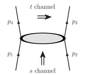
Figure 1: The $t$-channel exchange dominating the high-energy limit, $s\gg-t>0$. The figure also defines our conventions for momenta assignment and Mandelstam invariants. We shall assume that particles 2 and 3 (1 and 4) are of the same type and have the same helicity.

Let us consider a $2\to 2$ scattering amplitude ${\cal M}_{ij\to ij}$, where $i,j$ can be a quark or a gluon. The momenta are assigned as indicated in figure 1. In the following we will suppress the species indices $i,j$, unless explicitly needed. The high-energy limit corresponds to a configuration of forward scattering, such that the Mandelstam variables satisfy $s\gg-t>0$. In analysing this limit it is convenient to decompose the amplitude into its odd and even components with respect to $s\leftrightarrow u$ exchange, the so-called signature:

$${\cal M}^{(\pm)}(s,t)=\tfrac{1}{2}\Big{(}{\cal M}(s,t)\pm{\cal M}(-s-t,t)\Big{)},\\$$ (1)

where ${\cal M}^{(+)}$, ${\cal M}^{(-)}$ are referred to, respectively, as the even and odd amplitudes. As shown in ref. Caron-Huot:2017fxr , these have respectively real and imaginary coefficients, when expressed in terms of the natural signature-even combination of logarithms,

$$\frac{1}{2}\left(\log\frac{-s-i0}{-t}+\log\frac{-u-i0}{-t}\right)\simeq\log\left|\frac{s}{t}\right|-i\frac{\pi}{2}\equiv L,$$ (2)

and have independent factorisation properties in the high-energy limit. The effect we discuss in the following originates from the exchange of two Reggeons, therefore it proves useful to define a reduced amplitude, as introduced in ref. Caron-Huot:2017fxr , dividing by the effect of one-Reggeon exchange:

$$\hat{\mathcal{M}}_{ij\to ij}\equiv\,e^{-\,{\bf T}_{t}^{2}\,\alpha_{g}(t)\,L}\,\mathcal{M}_{ij\to ij}\,,$$ (3)

where ${\bf T}_{t}^{2}$ represents the total colour charge exchanged in the $t$ channel (see eq. (10) below). The function $\alpha_{g}(t)$ in eq. (3) represents the gluon Regge trajectory having the perturbative expansion

$$\alpha_{g}(t)\,=\,\sum_{n=1}^{\infty}\left(\frac{\alpha_{s}}{\pi}\right)^{n}\alpha^{(n)}_{g}(t)\,.$$ (4)

Given that we work to NLL accuracy, we will only need the gluon Regge trajectory to first order in $\alpha_{s}$, where in $d=4-2\epsilon$ dimensions

$$\alpha^{(1)}_{g}(t)\,=\,\frac{B_{0}(\epsilon)}{2\epsilon}\left(\frac{-t}{\mu^{2}}\right)^{-\epsilon}\,\,\stackrel{{\scriptstyle\mu^{2}\to-t}}{{=}}\,\,\frac{B_{0}(\epsilon)}{2\epsilon}\,.$$ (5)

Here, $B_{0}(\epsilon)$ is a ubiquitous loop factor and the first of a class of bubble integrals, cf. eq. (38), to become important in section 3. For now, it suffices to know that

$$B_{0}(\epsilon)=e^{\epsilon\gamma_{\rm E}}\frac{\Gamma^{2}(1-\epsilon)\Gamma(1+\epsilon)}{\Gamma(1-2\epsilon)}\,=\,1-\frac{\zeta_{2}}{2}\epsilon^{2}-\frac{7\zeta_{3}}{3}\epsilon^{3}+\ldots.$$ (6)

In the following we will consider the leading contributions to the signature-even amplitude to all orders, corresponding to the two-Reggeon exchange. These corrections — which we denote by ${\hat{\mathcal{M}}}_{\rm NLL}^{(+)}$ — were studied long ago Kuraev:1977fs ; Balitsky:1978ic and can be expressed in terms the two-Reggeized-gluon wavefunction $\Omega(p,k)$ as follows:

$${\hat{\mathcal{M}}}_{\rm NLL}^{(+)}\left(\frac{s}{-t}\right)=-i\pi\int[\mathrm{D}k]\,\frac{p^{2}}{k^{2}(p-k)^{2}}\,\Omega(p,k)\,{\bf T}_{s{-}u}^{2}\,{\cal M}^{(\text{tree})}_{ij\to ij}\,,$$ (7)

where the integration measure is

$$[\mathrm{D}k]\equiv\frac{\pi}{B_{0}}\,\left(\frac{\mu^{2}}{4\pi e^{-\gamma_{E}}}\right)^{\epsilon}\,\frac{\mathrm{d}^{2{-}2\epsilon}k}{(2\pi)^{2-2\epsilon}}\,.$$ (8)

with $B_{0}\equiv B_{0}(\epsilon)$ and the tree amplitude is

$${\cal M}^{(\text{tree})}_{ij\to ij}=4\pi\alpha_{s}\,\frac{2s}{t}(T_{i}^{b})_{a_{1}a_{4}}(T_{j}^{b})_{a_{2}a_{3}}\delta_{\lambda_{1}\lambda_{4}}\delta_{\lambda_{2}\lambda_{3}}\,,$$ (9)

where $\lambda_{i}$ for $i=1$ through $4$ are helicity indices. The colour operator ${\bf T}_{s{-}u}^{2}$ in eq. (7) acts on ${\cal M}^{(\text{tree})}_{ij\to ij}$ and it is defined in terms of the usual basis of Casimirs corresponding to colour flow through the three channels Dokshitzer:2005ig ; DelDuca:2011ae :

$${\bf T}_{s{-}u}^{2}\,\equiv\,\frac{{\bf T}_{s}^{2}-{\bf T}_{u}^{2}}{2},\qquad\rm{with}\qquad\left\{\begin{array}[]{c}{\bf T}_{s}={\bf T}_{1}+{\bf T}_{2}=-{\bf T}_{3}-{\bf T}_{4},\\ {\bf T}_{u}={\bf T}_{1}+{\bf T}_{3}=-{\bf T}_{2}-{\bf T}_{4},\\ {\bf T}_{t}={\bf T}_{1}+{\bf T}_{4}=-{\bf T}_{2}-{\bf T}_{3},\end{array}\right.\,$$ (10)

where ${\bf T}_{i}$ represent the colour charge operator Catani:1998bh in the representation corresponding to parton $i$. The wavefunction $\Omega(p,k)$ has a perturbative expansion in the strong coupling, taking the form

$$\Omega(p,k)=\sum_{\ell=1}^{\infty}\left(\frac{\alpha_{s}}{\pi}\right)^{\ell}L^{\ell-1}\frac{B_{0}^{\ell}}{(\ell-1)!}\,{\Omega}^{(\ell-1)}(p,k)\,,$$ (11)

where we set the renormalization scale equal to the momentum transfer, $\mu^{2}=-t=p^{2}$. The amplitude itself then has the corresponding expansion

$$\hat{\mathcal{M}}_{\rm NLL}^{(+)}\left(\frac{s}{-t}\right)=\sum_{\ell=1}^{\infty}\left(\frac{\alpha_{s}}{\pi}\right)^{\ell}\,L^{\ell-1}\,\hat{\mathcal{M}}_{\rm NLL}^{(+,\ell)}\,.$$ (12)

We emphasise that while these corrections are the leading-logarithmic contributions to the even amplitude, we denote them by NLL to recall that the power of the logarithm $L$ is one less than the loop order. This can be contrasted with the single-Reggeized-gluon contribution to the odd amplitude $\mathcal{M}_{\rm LL}^{(-)}\sim\,e^{\,{\bf T}_{t}^{2}\,\alpha_{g}(t)\,L}\,\mathcal{M}^{(\rm tree)}$.

In eq. (12) $\hat{\mathcal{M}}_{\rm NLL}^{(+,\ell)}$ contains $\ell$-loop diagrams and can be computed from the $(\ell-1)$-loop contribution to the wavefunction through integration

$$\hat{\mathcal{M}}_{\rm NLL}^{(+,\ell)}=-i\pi\frac{(B_{0})^{\ell}}{(\ell-1)!}\int[\mathrm{D}k]\,\frac{p^{2}}{k^{2}(p-k)^{2}}\,{\Omega}^{(\ell-1)}(p,k)\,{\bf T}_{s{-}u}^{2}\,\mathcal{M}^{(\rm tree)}\,.$$ (13)

In the normalisation used in eq. (13), the leading-order wavefunction is simply

$${\Omega}^{(0)}(p,k)=1.$$ (14)

At loop level the wavefunction is then obtained iteratively by applying the BFKL Hamiltonian:

$${\Omega}^{(\ell-1)}(p,k) = (2C_{A}-{\bf T}_{t}^{2})\,\int[\mathrm{D}k^{\prime}]\,f(p,k,k^{\prime})\,{\Omega}^{(\ell-2)}(p,k^{\prime})+\tilde{J}(p,k)\,{\Omega}^{(\ell-2)}(p,k)$$ (15)

$$\equiv \hat{H}\,{\Omega}^{(\ell-2)}(p,k)$$

where $f(p,k,k^{\prime})$ is the BFKL evolution kernel

$$f(p,k,k^{\prime})\equiv\frac{k^{2}}{k^{\prime 2}(k-k^{\prime})^{2}}+\frac{(p-k)^{2}}{(p-k^{\prime})^{2}(k-k^{\prime})^{2}}-\frac{p^{2}}{k^{\prime 2}(p-k^{\prime})^{2}},$$ (16)

and the function $\tilde{J}(p,k)$ is

$$\tilde{J}(p,k)=\frac{1}{2\epsilon}\left[C_{A}\left(\frac{p^{2}}{k^{2}}\right)^{\epsilon}+C_{A}\left(\frac{p^{2}}{(p-k)^{2}}\right)^{\epsilon}-{\bf T}_{t}^{2}\right]\,.$$ (17)

Eq. (15) is the standard BFKL Hamiltonian (see eq. (17) of the initial reference Kuraev:1977fs ) written using dimensional regularisation as an infrared regulator. $\tilde{J}(p,k)$ accounts for the Regge trajectories of the individual Reggeized gluons, minus the overall Regge trajectory with colour charge ${\bf T}_{t}^{2}$ which was subtracted in the exponent of the reduced amplitude (3).

As discussed in refs. Caron-Huot:2013fea ; Caron-Huot:2017fxr and briefly reviewed in appendix A, this equation and its higher-order generalisations can be understood by considering the expectation value of Wilson lines associated to the colour flow of the external partons Balitsky:1995ub , which are described as “target” and “projectile” in the (high-energy) forward scattering configuration of figure 1. The wavefunction then represents the transverse momenta in each of two Wilson lines and the BFKL equation is obtained as an appropriate limit of the more general Balitsky-JIMWLK evolution equation.

A graphical representation of eq. (13) is provided in figure 2. As a result of BFKL evolution, the amplitude at NLL accuracy can be represented as a ladder. At order $\ell$ it is obtained by closing the ladder and integrating the wavefunction of order $(\ell-1)$ over the resulting loop momentum, according to eq. (13). The wavefunction ${\Omega}^{(\ell-1)}(p,k)$, in turn, is obtained by applying once the leading-order BFKL evolution kernel to the wavefunction of order $(\ell-2)$. Graphically, this operation corresponds to adding one rung to the ladder.

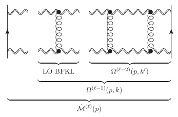
Figure 2: Graphical representation of the amplitude at NLL accuracy, as obtained through BFKL evolution. The addition of one rung corresponds to applying once the leading-order BFKL evolution onto the projectile wavefunction or impact factor at order $(\ell-2)$. This gives the wavefunction at order $(\ell-1)$, according to eq. (18). Closing the ladder and integrating over the resulting loop momentum gives the reduced amplitude, according to eq. (13).

2.2 Iterative solution for the wavefunction and amplitude

Eq. (13) shows that the $\ell$-th order amplitude is obtained in terms of iterated integrals, which arise upon evaluating the wavefunction ${\Omega}^{(\ell-1)}(p,k)$ to order $(\ell-1)$. It is straightforward to compute the first few orders, which gives us an opportunity to revisit the findings of ref. Caron-Huot:2013fea . We will be able to explain why a new colour structure emerges for the first time at four loops, and explore the general structure of the relevant iterated integrals.

A useful fact is that the evolution admits one well-known solution in the case where the exchanged state is colour-adjoint and $\Omega(p,k)$ is constant (independent of $k$) Kuraev:1977fs ; Balitsky:1978ic , which gives a positive-signature state with the same leading-order trajectory as the Reggeized gluon. This enables one to rewrite the Hamiltonian (15) as a part which vanishes when $\Omega(p,k)$ is constant, plus a part proportional to $(C_{A}-{\bf T}_{t}^{2})$:

$${\Omega}^{(\ell-1)}(p,k)=\hat{H}\,{\Omega}^{(\ell-2)}(p,k),\qquad\hat{H}=(2C_{A}-{\bf T}_{t}^{2})\,\hat{H}_{\rm i}+(C_{A}-{\bf T}_{t}^{2})\,\hat{H}_{\rm m}$$ (18)

where, explicitly,

$$\hat{H}_{\rm i}\,\Psi(p,k) = \int[\mathrm{D}k^{\prime}]\,f(p,k,k^{\prime})\Big{[}\Psi(p,k^{\prime})-\Psi(p,k)\Big{]},$$

$$\hat{H}_{\rm m}\,\Psi(p,k) = J(p,k)\,\Psi(p,k),$$ (19)

where the function $J(p,k)$ is defined by

$$J(p,k) =\frac{1}{2\epsilon}+\int[\mathrm{D}k^{\prime}]\,f(p,k,k^{\prime})$$

$$=\frac{1}{2\epsilon}\left[2-\left(\frac{p^{2}}{k^{2}}\right)^{\epsilon}-\left(\frac{p^{2}}{(p-k)^{2}}\right)^{\epsilon}\right].$$ (20)

The first interesting feature to note is that the $\hat{H}_{\rm i}$ operator in eq. (18) vanishes when acting on ${\Omega}^{(0)}(p,k)=1$. Therefore the wavefunction to one-loop involves a single colour structure:

$${\Omega}^{(1)}(p,k)=(C_{A}-{\bf T}_{t}^{2})\,J(p,k)\,.$$ (21)

The second colour structure appears for the first time at the second order:

$${\Omega}^{(2)}(p,k)=(C_{A}-{\bf T}_{t}^{2})^{2}\left(J(p,k)\right)^{2}+(2C_{A}-{\bf T}_{t}^{2})(C_{A}-{\bf T}_{t}^{2})\int[\mathrm{D}k^{\prime}]\,f(p,k,k^{\prime})\Big{[}J(p,k^{\prime})-J(p,k)\Big{]}\,.$$ (22)

Inserting the explicit form of $J(p,k)$ from eq. (2.2) into eq. (22), one finds that it involves bubble integrals, as well as three-mass triangle integrals with massless propagators, such as

$$\int[\mathrm{D}k^{\prime}]\,\frac{(p-k)^{2}}{(p-k^{\prime})^{2}(k-k^{\prime})^{2}}\left(\frac{p^{2}}{k^{\prime 2}}\right)^{\epsilon},$$ (23)

which is represented in figure 3.

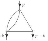
Figure 3: Three-mass triangle integral with massless propagators appearing in the calculation of the wavefunction at two loops. This type of integrals contribute to the amplitude only starting at four loops, due to the symmetry of the problem, as discussed in the main text. The bubble integral on one of the two edges of the triangles clarifies the origin of the propagator which is raised to power $\epsilon$ in eq. (23).

The wavefunction at higher orders can be expressed formally by introducing a class of functions

$$\Omega_{\rm ia_{1}\ldots a_{n}}(p,k) \equiv \int[\mathrm{D}k^{\prime}]\,f(p,k,k^{\prime})\Big{[}\Omega_{\rm a_{1}\ldots a_{n}}(p,k^{\prime})-\Omega_{\rm a_{1}\ldots a_{n}}(p,k)\Big{]}\,,$$

$$\Omega_{\rm ma_{1}\ldots a_{n}}(p,k) \equiv J(p,k)\,\Omega_{\rm a_{1}\ldots a_{n}}(p,k)\,,$$ (24)

where $\Omega_{\varnothing}(p,k)\equiv 1$, and each of the indices ${\rm a_{j}}$ can take the value “i” or “m”, which stand for integration and multiplication, respectively, according to the action of the two Hamiltonian operators in eq. (2.2). In this notation, the one- and two-loop wavefunctions read, respectively,

$${\Omega}^{(1)}(p,k) = (C_{A}-{\bf T}_{t}^{2})\,\Omega_{\rm m}\,,$$

$${\Omega}^{(2)}(p,k) = (C_{A}-{\bf T}_{t}^{2})^{2}\,\Omega_{\rm mm}+(2C_{A}-{\bf T}_{t}^{2})(C_{A}-{\bf T}_{t}^{2})\,\Omega_{\rm im}\,,$$ (25)

and it is also easy to write the wavefunctions at higher loops, for example:

$${\Omega}^{(3)}(p,k) = (C_{A}-{\bf T}_{t}^{2})^{3}\,\Omega_{\rm mmm}+(2C_{A}-{\bf T}_{t}^{2})(C_{A}-{\bf T}_{t}^{2})^{2}\big{(}\Omega_{\rm imm}+\Omega_{\rm mim}\big{)}$$ (26)

$$+ (2C_{A}-{\bf T}_{t}^{2})^{2}(C_{A}-{\bf T}_{t}^{2})\,\Omega_{\rm iim}\,.$$

The wavefunctions written thus far are sufficient to evaluate the reduced amplitude up to four loops. At one and two loops, inserting respectively ${\Omega}^{(0)}(p,k)=1$ and eq. (21) into eq. (13) and performing bubble integrals one gets immediately

$$\hat{\mathcal{M}}_{\rm NLL}^{(+,1)} = -i\pi\,\frac{B_{0}}{2\epsilon}\,{\bf T}_{s{-}u}^{2}\,\mathcal{M}^{(\rm tree)},$$ (27)

$$\hat{\mathcal{M}}_{\rm NLL}^{(+,2)} = i\pi\,\frac{(B_{0})^{2}}{2}\left[\frac{1}{(2\epsilon)^{2}}+\frac{9\zeta_{3}}{2}\epsilon+\frac{27\zeta_{4}}{4}\epsilon^{2}+\frac{63\zeta_{5}}{2}\epsilon^{3}+{\cal O}(\epsilon^{4})\right]\,(C_{A}-{\bf T}_{t}^{2})\,{\bf T}_{s{-}u}^{2}\,\mathcal{M}^{(\rm tree)}.$$

We notice that the amplitude depends solely on the colour structure $(C_{A}-{\bf T}_{t}^{2})$, and this in turn is a consequence of the fact that the wavefunctions ${\Omega}^{(0)}$ and ${\Omega}^{(1)}$ have only one colour component. Based on this consideration alone, one would expect the second colour structure, $(2C_{A}-{\bf T}_{t}^{2})$, to contribute to the amplitude starting at three loops, given that it appears in ${\Omega}^{(2)}(p,k)$ of eq. (2.2). However, this contribution of ${\Omega}^{(2)}(p,k)$ to the amplitude $\hat{\mathcal{M}}_{\rm NLL}^{(+,3)}$ cancels by symmetry:

$$\int[\mathrm{D}k]\,\frac{p^{2}}{k^{2}(p-k)^{2}}\,\Omega_{\rm im}(p,k) = \int[\mathrm{D}k]\,[\mathrm{D}k^{\prime}]\,\frac{p^{2}}{k^{2}(p-k)^{2}}\,f(p,k,k^{\prime})\Big{[}J(p,k^{\prime})-J(p,k)\Big{]}$$ (28)

$$=\,\int[\mathrm{D}k]\,[\mathrm{D}k^{\prime}]\bigg{\{}\frac{p^{2}}{k^{\prime 2}(p-k^{\prime})^{2}}\,f(p,k^{\prime},k)J(p,k^{\prime})-(k\leftrightarrow k^{\prime})\bigg{\}}=0,$$

where in the last line we used the property

$$\frac{p^{2}}{k^{\prime 2}(p-k^{\prime})^{2}}\,f(p,k^{\prime},k)=\frac{p^{2}}{k^{2}(p-k)^{2}}\,f(p,k,k^{\prime}),$$ (29)

which makes evident that eq. (28) vanishes by antisymmetry with respect to $k\leftrightarrow k^{\prime}$. Because of this, the amplitude at three loops has again a single colour component, proportional to $(C_{A}-{\bf T}_{t}^{2})^{2}$:

$$\hat{\mathcal{M}}_{\rm NLL}^{(+,3)}=i\pi\,\frac{(B_{0})^{3}}{3!}\left[\frac{1}{(2\epsilon)^{3}}-\frac{11\zeta_{3}}{4}-\frac{33\zeta_{4}}{8}\epsilon-\frac{357\zeta_{5}}{4}\epsilon^{2}+{\cal O}(\epsilon^{3})\right]\,(C_{A}-{\bf T}_{t}^{2})^{2}\,{\bf T}_{s{-}u}^{2}\,\mathcal{M}^{(\rm tree)}.$$ (30)

This symmetry relation generalises to higher orders, i.e. one has

$$\int[\mathrm{D}k]\,\frac{p^{2}}{k^{2}(p-k)^{2}}\Omega_{\rm ia_{1}\ldots a_{n}}(p,k)=0,$$ (31)

for any ${\rm a_{1}\ldots a_{n}}$. While this symmetry ensures that there is only one colour structure at three loops, this is no longer the case starting at four loops. There, one obtains Caron-Huot:2013fea

$$\hat{\mathcal{M}}_{\rm NLL}^{(+,4)} = -i\pi\frac{(B_{0})^{4}}{3!}\int[\mathrm{D}k]\frac{p^{2}}{k^{2}(p-k)^{2}}\bigg{\{}(C_{A}-{\bf T}_{t}^{2})^{3}\,\Omega_{\rm mmm}(p,k)$$

$$\hskip 113.81102pt+\,(2C_{A}-{\bf T}_{t}^{2})(C_{A}-{\bf T}_{t}^{2})^{2}\,\Omega_{\rm mim}(p,k)\bigg{\}}\,{\bf T}_{s{-}u}^{2}\,\mathcal{M}^{(\rm tree)}$$

$$= i\pi\,\frac{(B_{0})^{4}}{4!}\bigg{\{}(C_{A}-{\bf T}_{t}^{2})^{3}\bigg{(}\frac{1}{(2\epsilon)^{4}}+\frac{175\zeta_{5}}{2}\epsilon+{\cal O}(\epsilon^{2})\bigg{)}$$

$$\hskip 25.6073pt+\,C_{A}(C_{A}-{\bf T}_{t}^{2})^{2}\bigg{(}-\frac{\zeta_{3}}{8\epsilon}-\frac{3}{16}\zeta_{4}-\frac{167\zeta_{5}}{8}\epsilon+{\cal O}(\epsilon^{2})\bigg{)}\bigg{\}}\,{\bf T}_{s{-}u}^{2}\,\mathcal{M}^{(\rm tree)}.$$

One sees that the integrated result involves two colour structures, and in the final expression in eq. (2.2) we rearranged them so as to single out a factor of $C_{A}$. In section 4 below we will see that in this form it is easy to compare the amplitude with the structure of infrared divergences. Specifically, we will see that corrections involving the colour structure $(C_{A}-{\bf T}_{t}^{2})^{\ell-1}$ at $\ell$ loop order emerge directly from the simplest “dipole” formula of the soft anomalous dimension, while other colour structures, namely $C_{A}^{j}(C_{A}-{\bf T}_{t}^{2})^{\ell-j-1}$ with $j\geq 1$, identify deviations from the dipole formula, as was first observed in ref. Caron-Huot:2013fea for $\ell=4$.

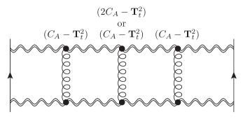
Figure 4: Graphical representation of the BFKL ladder at four loops. The fact that ${\Omega}^{(1)}(p,k)\sim(C_{A}-{\bf T}_{t}^{2})$ in conjunction with the target-projectile symmetry imply that the first rungs on either side can only give rise to contributions proportional to $(C_{A}-{\bf T}_{t}^{2})$. As a consequence, distinct colour structures can appear for the first time at four loops.

Inspecting the diagrammatic representation of BFKL evolution in figure 2, one can interpret the delayed appearance of a new colour structure to four loops, as a consequence of the target-projectile symmetry. Recall that for the first rung of the ladder, only the second term $\hat{H}_{\rm m}$ in eq. (18) contributes, so the wavefunction has a single colour structure $(C_{A}-{\bf T}_{t}^{2})$. Considering more rungs, using target-projectile symmetry one can deduce that the same is true for the first rung on the opposite side of the ladder. As a consequence, despite the fact that ${\Omega}^{(2)}(p,k)$ contains two structures (see eq. (2.2)), the effect of the second one, $(2C_{A}-{\bf T}_{t}^{2})$, cannot appear in the three-loop amplitude, where each of the two rungs contribute a factor of $(C_{A}-{\bf T}_{t}^{2})$. As shown in figure 4, distinct colour structures can only appear in the amplitude starting at four loops, where the middle rung — and only that rung — gives rise to both colour factors.

3 The soft approximation

While it would be possible to calculate the wavefunction and amplitude to higher loop orders, in this paper we focus on the infrared divergent part of the latter. We strive to compare its singularities with the predictions made by the infrared factorisation theorem and, consequently, deduce higher-order corrections to the high-energy soft anomalous dimension. With this goal in mind, we highlight at this point another important property of $\Omega(p,k)$, which can be verified when inspecting eq. (18) more carefully (see below): the wavefunction $\Omega^{(\ell-1)}(p,k)$ is finite for $\epsilon\to 0$ to all orders in perturbation theory! This is a non-trivial statement, which becomes evident only after the evolution evolution equation is brought from the form in eq. (15) to eq. (18). A practical implication is that all divergences in the amplitude must originate in the final integration, namely going from the wavefunction to the amplitude as in eq. (7). Inspecting the latter equation, we see that divergences arise only in the $k\to 0$ and $k\to p$ limits (and ultraviolet power counting in eq. (2.2) using (16) excludes divergences from $k^{\prime}\gg p,k$). Due to the symmetry of the integrand, all divergences of the amplitude can therefore be obtained by evaluating it in one of these two limits, and multiplying the result by two.

Let us now examine more carefully the evolution of the wavefunction according to eqs. (18) and (2.2), verify that the wavefunction is indeed finite, and derive a simplified version of the evolution, valid in the small-$k$ or soft approximation: $k\ll p$. The loop integral in eq. (2.2) can in principle receive contributions from two regions; $k\ll k^{\prime}\sim p$ and $k\sim k^{\prime}\ll p$. Inspecting the form of $f(p,k,k^{\prime})$ in the two regions, it is easy to check that only the second region contributes:

$$f(p,k,k^{\prime})|_{k\ll k^{\prime}\sim p} \longrightarrow 0+\frac{p^{2}}{(p-k^{\prime})^{2}k^{\prime 2}}-\frac{p^{2}}{k^{\prime 2}(p-k^{\prime})^{2}}\,=\,0,$$

$$f(p,k,k^{\prime})|_{k\sim k^{\prime}\ll p} \longrightarrow \frac{k^{2}}{k^{\prime 2}(k-k^{\prime})^{2}}+\frac{1}{(k-k^{\prime})^{2}}-\frac{1}{k^{\prime 2}}=\frac{2(k\cdot k^{\prime})}{k^{\prime 2}(k-k^{\prime})^{2}}.$$ (33)

This means that the soft approximation closes under evolution! In the following, we will identify the region $k\sim k^{\prime}\ll p$ as soft and add a subscript $s$ to quantities calculated in this limit. From $J(p,k)$ in eq. (2.2) one gets

$$J_{s}(p,k)=\frac{1}{2\epsilon}\left[1-\left(\frac{p^{2}}{k^{2}}\right)^{\epsilon}\,\right],$$ (34)

and the evolution in eq. (18) becomes

$$\Omega^{(\ell-1)}_{s}(p,k) = \hat{H}_{s}\,\Omega^{(\ell-2)}_{s}(p,k)\,,$$

$$\hat{H}_{s}\Psi(p,k) = (2C_{A}-{\bf T}_{t}^{2})\int[\mathrm{D}k^{\prime}]\frac{2(k\cdot k^{\prime})}{k^{\prime 2}(k-k^{\prime})^{2}}\,\Big{[}\Psi(p,k^{\prime})-\Psi(p,k)\Big{]}$$ (35)

$$+\,(C_{A}-{\bf T}_{t}^{2})\,J_{s}(p,k)\,\Psi(p,k)\,,$$

where $[\mathrm{D}k^{\prime}]$ is the previously defined integration measure (8). Eq. (35) confirms that it is consistent to truncate the Regge evolution to the soft approximation: using the power counting $\Psi(p,k)\sim 1$, we see that the $k^{\prime}$ integral is saturated by the soft region $k^{\prime}\sim k$, with no sensitivity to larger scales.

Inserting the wavefunction $\Omega_{s}^{(\ell-1)}(p,k)$ into eq. (13), we get the amplitude in the soft limit at the $\ell$-th order. In this approximation the last integral becomes divergent and needs an ultraviolet cutoff, which we fix by requiring $k^{2}<p^{2}$, based on dimensional analysis and consistency with the soft limit (any cutoff would be consistent, and would not affect the infrared singularities). The integration measure for the last integral therefore reads

$$\int[Dk]_{s}=\frac{(p^{2})^{\epsilon}\,e^{\epsilon\gamma_{E}}}{2\Gamma(1-\epsilon)B_{0}}\int_{0}^{p^{2}}\mathrm{d}k^{2}(k^{2})^{-\epsilon},$$ (36)

where we multiplied by a factor of two, in order to take into account the fact that there is an identical contribution from the region where the Reggeized gluon carrying momentum $(p-k)$ is soft. Inserting this result into eq. (13), we get $\hat{\mathcal{M}}_{\rm NLL}^{(+,\ell)}$ in the soft approximation:

$$\hat{\mathcal{M}}_{\rm NLL}^{(+,\ell)}=-\frac{i\pi(B_{0})^{\ell-1}}{(\ell-1)!}\,\frac{e^{\epsilon\gamma_{E}}}{\Gamma(1-\epsilon)}\int_{0}^{p^{2}}\frac{\mathrm{d}k^{2}}{2k^{2}}\,\left(\frac{p^{2}}{k^{2}}\right)^{\epsilon}\,{\Omega}_{s}^{(\ell-1)}(p,k)\,{\bf T}_{s{-}u}^{2}\,\mathcal{M}^{(\rm tree)}+{\cal O}(\epsilon^{0}).$$ (37)

We stress that this approximation gives correct results only as far as infrared singularities are concerned. All poles in $\epsilon$ are exact, since the integrand is finite and divergences arise only from the $k\to 0$ limit of integration. The reduced amplitude in eq. (37) ceases to be correct at finite ${\cal O}(\epsilon^{0})$ order, as indicated.

The most significant advantage of the soft approximation is that the evolution equation greatly simplifies, and this allows us to obtain closed-form expressions for the wavefunction ${\Omega}_{s}^{(\ell-1)}(p,k)$ and the amplitude $\hat{\mathcal{M}}_{\rm NLL}^{(+,\ell)}|_{s}$, as we are going to detail in the following.

3.1 The wavefunction at NLL to all orders

In analogy to the exercise done in section 2.2, we start by calculating explicitly the wavefunction at the first few orders in perturbation theory, this time in the soft approximation. The initial condition is still given by eq. (14), and the evolution obeys eq. (35). This equation has a much simpler structure compared to the original one, eq. (2.2), because the soft approximation turns a two-scale problem into a one-scale problem. It is easy to check that the wavefunction reduces to a polynomial in $\xi=\left(p^{2}/k^{2}\right)^{\epsilon}$, which implies that the integrals involved in eq. (35) are simple bubble integrals of the type

$$\int[\mathrm{D}k^{\prime}]\,\frac{2(k\cdot k^{\prime})}{k^{\prime 2}(k-k^{\prime})^{2}}\,\left(\frac{p^{2}}{k^{\prime 2}}\right)^{n\epsilon}=-\frac{1}{2\epsilon}\frac{B_{n}(\epsilon)}{B_{0}(\epsilon)}\left(\frac{p^{2}}{k^{2}}\right)^{(n+1)\epsilon}\,,$$ (38)

where the integration measure is given in eq. (8). This defines a class of one-loop functions mentioned above eq. (6), namely

$$B_{n}(\epsilon)=e^{\epsilon\gamma_{\rm E}}\frac{\Gamma(1-\epsilon)}{\Gamma(1+n\epsilon)}\frac{\Gamma(1+\epsilon+n\epsilon)\Gamma(1-\epsilon-n\epsilon)}{\Gamma(1-2\epsilon-n\epsilon)}\,.$$ (39)

Using this we can write the action of the soft Hamiltonian (35) on any monomial ($m\geq 0$):

$$\hat{H}_{s}\,\xi^{m} = \frac{\xi^{m}}{2\epsilon}\left((1-\xi)(C_{A}-{\bf T}_{t}^{2})+\xi\hat{B}_{m}(\epsilon)(2C_{A}-{\bf T}_{t}^{2})\right)\,$$

$$= \frac{(C_{A}-{\bf T}_{t}^{2})}{2\epsilon}\left(\xi^{m}-\xi^{m+1}\left[1-\hat{B}_{m}(\epsilon)\frac{2C_{A}-{\bf T}_{t}^{2}}{C_{A}-{\bf T}_{t}^{2}}\right]\right)\,,$$

where we have introduced the loop functions

$$\hat{B}_{n}(\epsilon)=1-\frac{B_{n}(\epsilon)}{B_{0}(\epsilon)}\,=\,2n(2+n)\zeta_{3}\epsilon^{3}+3n(2+n)\zeta_{4}\epsilon^{4}+\ldots.$$ (41)

Given that $\hat{B}_{m}(\epsilon)={\cal O}(\epsilon^{3})$, the first line in eq. (3.1) makes manifest the fact that $\hat{H}_{s}\,\xi^{m}$ is finite for $\epsilon\to 0$, in line with our earlier assertion about the finiteness of the wavefunction. The second line will be useful in what follows for determining the all-order structure of the wavefunction.

Applying eq. (38) repeatedly up to three loops (which is sufficient to determine the amplitude at four loops) we find

$${\Omega}_{s}^{(0)}(\xi) = 1,$$ (42)

$${\Omega}_{s}^{(1)}(\xi) = \frac{(C_{A}-{\bf T}_{t}^{2})}{2\epsilon}\Big{(}1-\xi\Big{)},$$

$${\Omega}_{s}^{(2)}(\xi) = \frac{(C_{A}-{\bf T}_{t}^{2})^{2}}{(2\epsilon)^{2}}\bigg{\{}1-2\xi+\xi^{2}\left[1-\hat{B}_{1}(\epsilon)\frac{2C_{A}-{\bf T}_{t}^{2}}{C_{A}-{\bf T}_{t}^{2}}\right]\bigg{\}}\,,$$

$${\Omega}_{s}^{(3)}(\xi) = \frac{(C_{A}-{\bf T}_{t}^{2})^{3}}{(2\epsilon)^{3}}\bigg{\{}1-3\xi+3\xi^{2}\left[1-\hat{B}_{1}(\epsilon)\frac{2C_{A}-{\bf T}_{t}^{2}}{C_{A}-{\bf T}_{t}^{2}}\right]$$

$$\hskip 71.13188pt-\,\xi^{3}\left[1-\hat{B}_{1}(\epsilon)\frac{2C_{A}-{\bf T}_{t}^{2}}{C_{A}-{\bf T}_{t}^{2}}\right]\left[1-\hat{B}_{2}(\epsilon)\frac{2C_{A}-{\bf T}_{t}^{2}}{C_{A}-{\bf T}_{t}^{2}}\right]\bigg{\}}.$$

The evaluation of a few additional orders allows us to obtain an ansatz for the $(\ell-1)$-th order wavefunction:

$${\Omega}_{s}^{(\ell-1)}(p,k)=\frac{(C_{A}-{\bf T}_{t}^{2})^{\ell-1}}{(2\epsilon)^{\ell-1}}\sum_{n=0}^{\ell-1}(-1)^{n}\binom{\ell-1}{n}\left(\frac{p^{2}}{k^{2}}\right)^{n\epsilon}\prod_{m=0}^{n-1}\left\{1-\hat{B}_{m}(\epsilon)\frac{2C_{A}-{\bf T}_{t}^{2}}{C_{A}-{\bf T}_{t}^{2}}\right\}\,.$$ (43)

The validity of this all-order formula can be proved directly using the action of the Hamiltonian in the second line of eq. (3.1) by noticing first that, independently of the loop order, the term $\xi^{n}$ can only be generated by acting $n$ times with the second term of eq. (3.1), each of which raises the power of $\xi$ by one. Hence $\xi^{n}$ will always be accompanied by the product $(-1)^{n}\prod_{m=0}^{n-1}\left\{1-\hat{B}_{m}(\epsilon)\frac{2C_{A}-{\bf T}_{t}^{2}}{C_{A}-{\bf T}_{t}^{2}}\right\}$. Furthermore, the combinatorial factor $\binom{\ell-1}{n}$ associated with $\xi^{n}$ simply counts the number of different ways of acting $(\ell-1)$ times with the Hamiltonian, out of which $n$ times with the second term and $\ell-1-n$ times with the first.

3.2 The all-order structure of two-parton scattering amplitudes at NLL

The main result of the previous section is that, in the soft approximation, the wavefunction reduces to a polynomial in $\left(p^{2}/k^{2}\right)^{\epsilon}$, given by eq. (43). As a consequence, the calculation of the amplitude (37) becomes straightforward, because it involves only integrals of the type

$$\int_{0}^{p^{2}}\frac{\mathrm{d}k^{2}}{k^{2}}\,\left(\frac{p^{2}}{k^{2}}\right)^{n\,\epsilon}=-\frac{1}{n\,\epsilon},$$ (44)

which allows us to obtain

$$\left.\hat{\mathcal{M}}_{\rm NLL}^{(+,\ell)}\right|_{s}=i\pi\,\frac{1}{(2\epsilon)^{\ell}}\,\frac{B_{0}^{\ell}(\epsilon)}{\ell!}\,(1-\hat{B}_{-1})\,(C_{A}-{\bf T}_{t}^{2})^{\ell-1}\sum_{n=1}^{\ell}(-1)^{n+1}\,\binom{\ell}{n}\\ \times\prod_{m=0}^{n-2}\bigg{[}1-\hat{B}_{m}(\epsilon)\frac{2C_{A}-{\bf T}_{t}^{2}}{C_{A}-{\bf T}_{t}^{2}}\bigg{]}\,{\bf T}_{s{-}u}^{2}\,\mathcal{M}^{(\rm tree)}+{\cal O}(\epsilon^{0}),$$ (45)

where the factor $(1-\hat{B}_{-1})$ follows from rewriting the factor $e^{\epsilon\gamma_{E}}/\Gamma(1-\epsilon)=B_{-1}(\epsilon)$:

$$(B_{0})^{\ell-1}\,\frac{e^{\epsilon\gamma_{E}}}{\Gamma(1-\epsilon)}=(B_{0})^{\ell}\frac{B_{-1}(\epsilon)}{B_{0}(\epsilon)}=(B_{0})^{\ell}(1-\hat{B}_{-1}).$$ (46)

Eq. (45) looks rather involved but one must keep in mind that, upon expansion in $\epsilon$, it contains many finite terms which do not represent the actual amplitude since we are working in the soft approximation. Given the overall factor of $1/(2\epsilon)^{\ell}$ in eq. (45), all the singularities are obtained by retaining only contributions up to $\epsilon^{\ell-1}$ in the subsequent factors. When this is taken into account a great simplification arises: indeed, as shown in appendix B, it is possible to prove that eq. (45) is equivalent to

$$\left.\hat{\mathcal{M}}_{\rm NLL}^{(+,\ell)}\right|_{s}=i\pi\,\frac{1}{(2\epsilon)^{\ell}}\,\frac{B_{0}^{\ell}(\epsilon)}{\ell!}\,(1-\hat{B}_{-1})\left(1-\hat{B}_{-1}(\epsilon)\frac{2C_{A}-{\bf T}_{t}^{2}}{C_{A}-{\bf T}_{t}^{2}}\right)^{-1}\\ \times(C_{A}-{\bf T}_{t}^{2})^{\ell-1}\,{\bf T}_{s{-}u}^{2}\,\mathcal{M}^{(\rm tree)}+{\cal O}(\epsilon^{0}).$$ (47)

It is remarkable that the complicated sum of products of bubble integrals weighed by a binomial factor collapses to a single factor which depends only on one bubble integral, namely $\hat{B}_{-1}(\epsilon)$. The main ingredient of the proof is the fact that the wavefunction itself is finite.

Eq. (47) constitutes the main result of this section: by iterating the BFKL equation (which was not diagonalised before in $d=4-2\epsilon$ dimensions) we obtained the singular part of the even amplitude at NLL accuracy, to all orders in the strong coupling constant. Anticipating comparison with the structure of infrared divergences dictated by the soft anomalous dimension, it proves useful to rearrange eq. (47) in such a way to single out the colour structures $C_{A}$ and $(C_{A}-{\bf T}_{t}^{2})$. Indeed, as discussed at the end of section 2.2, we know that the dipole formula of infrared divergencies fixes the singularities of the even amplitude in the high-energy limit to be proportional to the colour structure $(C_{A}-{\bf T}_{t}^{2})^{\ell-1}{\bf T}_{s{-}u}^{2}$ at $\ell$ loops. From eq. (47) we obtain

$$\left.\hat{\mathcal{M}}_{\rm NLL}^{(+,\ell)}\right|_{s}=i\pi\,\frac{1}{(2\epsilon)^{\ell}}\,\frac{B_{0}^{\ell}(\epsilon)}{\ell!}\,\left(1-R(\epsilon)\frac{C_{A}}{C_{A}-{\bf T}_{t}^{2}}\right)^{-1}(C_{A}-{\bf T}_{t}^{2})^{\ell-1}\,{\bf T}_{s{-}u}^{2}\,\mathcal{M}^{(\rm tree)}+{\cal O}(\epsilon^{0}),$$ (48)

where we have introduced the function

$$R(\epsilon)\equiv\frac{B_{0}(\epsilon)}{B_{-1}(\epsilon)}-1 = \frac{\Gamma^{3}(1-\epsilon)\Gamma(1+\epsilon)}{\Gamma(1-2\epsilon)}-1$$ (49)

$$= -2\zeta_{3}\,\epsilon^{3}-3\zeta_{4}\,\epsilon^{4}-6\zeta_{5}\epsilon^{5}-\left(10\zeta_{6}-2\zeta^{2}_{3}\right)\epsilon^{6}+{\cal O}(\epsilon^{7}).$$

Furthermore, by resumming eq. (48) according to eq. (12) we get the all-order amplitude:

$$\left.\hat{\mathcal{M}}_{\mathrm{NLL}}^{(+)}\right|_{s}=\frac{i\pi}{L(C_{A}-{\bf T}_{t}^{2})}\left(1-R(\epsilon)\frac{C_{A}}{C_{A}-{\bf T}_{t}^{2}}\right)^{-1}\\ \times\left[\exp\left\{\frac{B_{0}(\epsilon)}{2\epsilon}\frac{\alpha_{s}}{\pi}L(C_{A}-{\bf T}_{t}^{2})\right\}-1\right]{\bf T}_{s{-}u}^{2}\,\mathcal{M}^{(\rm tree)}+{\cal O}(\epsilon^{0}).$$ (50)

This result will be used in the next section to extract the soft anomalous dimension.

Before addressing this topic, however, it proves useful to explore in more detail the implications of eq. (48) by writing explicitly a few orders in perturbation theory. Up to three loops eq. (48) reduces to

$$\left.\hat{\mathcal{M}}_{\rm NLL}^{(+,\ell=1,2,3)}\right|_{s}=i\pi\,\frac{B_{0}^{\ell}(\epsilon)}{\ell!\,(2\epsilon)^{\ell}}\,(C_{A}-{\bf T}_{t}^{2})^{\ell-1}\,{\bf T}_{s{-}u}^{2}\,\mathcal{M}^{(\rm tree)}+{\cal O}(\epsilon^{0}),$$ (51)

i.e. only one colour structure contributes to the amplitude up to three loops, and the singularities are correctly reproduced by the dipole formula of infrared divergences. Starting at four loops, and for the subsequent three orders, one gets an additional contribution proportional to a new colour structure:

$$\left.\hat{\mathcal{M}}_{\rm NLL}^{(+,\ell=4,5,6)}\right|_{s}=i\pi\,\frac{B_{0}^{\ell}(\epsilon)}{\ell!\,(2\epsilon)^{\ell}}\bigg{\{}(C_{A}-{\bf T}_{t}^{2})^{\ell-1}+R(\epsilon)\,C_{A}(C_{A}-{\bf T}_{t}^{2})^{\ell-2}\bigg{\}}\,{\bf T}_{s{-}u}^{2}\,\mathcal{M}^{(\rm tree)}+{\cal O}(\epsilon^{0}),$$ (52)

which matches with the infrared-divergent part of the result reported earlier in eq. (2.2). It can be easily verified (see the next section) that the infrared divergences associated with the first colour structure are predicted by the dipole formula, while the ones associated with the second are not. Next, starting at seven loops, and for the subsequent three orders, yet another colour structure arises:

$$\left.\hat{\mathcal{M}}_{\rm NLL}^{(+,\ell=7,8,9)}\right|_{s} = i\pi\,\frac{B_{0}^{\ell}(\epsilon)}{\ell!\,(2\epsilon)^{\ell}}\bigg{\{}(C_{A}-{\bf T}_{t}^{2})^{\ell-1}+R(\epsilon)\,C_{A}(C_{A}-{\bf T}_{t}^{2})^{\ell-2}$$

$$\hskip 56.9055pt+\,R^{2}(\epsilon)\,C_{A}^{2}(C_{A}-{\bf T}_{t}^{2})^{\ell-3}\bigg{\}}\,{\bf T}_{s{-}u}^{2}\,\mathcal{M}^{(\rm tree)}+{\cal O}(\epsilon^{0})\,.$$

Expanding eq. (48) for the next three orders in $\alpha_{s}$ we get

$$\left.\hat{\mathcal{M}}_{\rm NLL}^{(+,\ell=10,11,12)}\right|_{s} = i\pi\,\frac{B_{0}^{\ell}(\epsilon)}{\ell!\,(2\epsilon)^{\ell}}\bigg{\{}(C_{A}-{\bf T}_{t}^{2})^{\ell-1}+R(\epsilon)\,C_{A}(C_{A}-{\bf T}_{t}^{2})^{\ell-2}$$

$$+\,R^{2}(\epsilon)\,C_{A}^{2}(C_{A}-{\bf T}_{t}^{2})^{\ell-3}+R^{3}(\epsilon)\,C_{A}^{3}(C_{A}-{\bf T}_{t}^{2})^{\ell-4}\bigg{\}}\,{\bf T}_{s{-}u}^{2}\,\mathcal{M}^{(\rm tree)}+{\cal O}(\epsilon^{0})\,.$$

It is now easy to understand the pattern singularities implied by eq. (48): at each order the first colour structure, proportional to $(C_{A}-{\bf T}_{t}^{2})^{\ell-1}$, describes the singularities predicted by the dipole formula. Additional colour structures are generated by the expansion of the geometric series $1/\left(1-R(\epsilon)\frac{C_{A}}{C_{A}-{\bf T}_{t}^{2}}\right)$ in eq. (48), such that every three loops a new colour structure arises with an increasing power of $C_{A}$, replacing one of the factors of $(C_{A}-{\bf T}_{t}^{2})$. All these new structures introduce infrared divergences, which are not accounted for by the dipole formula.

Now that we understand the result implied by the BFKL evolution equation, we are in the position to investigate how the infrared divergences not accounted for by the dipole formula can be included in the soft anomalous dimension. This will be the subject of the following section.

4 The soft anomalous dimension in the high-energy limit to all orders

It is well known that infrared divergences in gauge-theory scattering amplitudes are multiplicatively “renormalizable”: finite hard-scattering amplitudes may be obtained by multiplying the original infrared-divergent amplitude by a renormalization factor ${\bf Z}(\{p_{i}\},\mu,\alpha_{s}(\mu))$, which is matrix-valued in colour-flow space. This factor solves a renormalization group equation, and hence can be written as a path-ordered exponential of a soft anomalous dimension ${\bf\Gamma}(\{p_{i}\},\mu,\alpha_{s}(\mu))$, integrated over the scale $\mu$. As such, the soft anomalous dimension constitutes a fundamental ingredient for the calculation of scattering processes at any given order in perturbation theory, and much effort has been devoted to its determination. It has been shown that the soft anomalous dimension has a simple dipole structure up to two loops Aybat:2006mz . Corrections involving three and four partons arise starting at three loops, and a series of analyses has been performed in order to constrain their structure at three loops and beyond Becher:2009cu ; Gardi:2009qi ; Becher:2009qa ; Gardi:2009zv ; Dixon:2009ur ; Ahrens:2012qz ; the complete correction at three loops was calculated recently Almelid:2015jia ; Gardi:2016ttq .

The general structure of the soft anomalous dimension is fixed by the factorisation properties of soft and collinear radiation, along with symmetry properties, such as rescaling invariance of soft corrections with respect to the momenta of the hard partons. The latter properties link dipole terms to the cusp anomalous dimension and dictate the structure of corrections to the soft anomalous dimension that correlate more than two partons Becher:2009cu ; Gardi:2009qi ; Becher:2009qa ; Gardi:2009zv . In particular, they imply that at three loops, non-dipole corrections can only depend on the kinematics via rescaling-invariant cross ratios. The soft anomalous dimension can be further constrained by the behaviour of scattering amplitudes in special kinematic limits, such as the Regge limit Bret:2011xm ; DelDuca:2011ae ; Caron-Huot:2017fxr and collinear limits Becher:2009cu ; Dixon:2009ur . Furthermore, it was recently shown Almelid:2017qju that the space of functions in terms of which the non-dipole correction is expressed (single-valued multiple polylogarithms) can, in fact, be deduced from general considerations. A bootstrap procedure was then set up, which remarkably completely fixes the functional form of the non-dipole correction at three loops (up to an overall rational numerical factor) based on known information from the kinematic limits mentioned above, reproducing the result of the Feynman-diagram computation of ref. Almelid:2015jia ; Gardi:2016ttq . The prospects of extending this bootstrap procedure to higher loops provides an additional motivation to determining the soft anomalous dimension in the high-energy limit.

As discussed above, ref. Caron-Huot:2013fea determined the next-to-leading high-energy logarithms (NLL) of $2\to 2$ scattering amplitudes at four loops. In this paper we have been able to extend this and computed the infrared singularities at NLL in the high-energy limit to all order in perturbation theory. We are therefore able to determine the soft anomalous dimension in this approximation to all orders.

We start this section by briefly reviewing the structure of the soft anomalous dimension in the high-energy limit, and then determine it to all orders by extracting the ${\cal O}(1/\epsilon)$ coefficient from the amplitude obtained in section 3.2, which we then analyze numerically in detail. Finally we show that the singularity structure we deduced from the high-energy limit computation, consisting of poles of ${\cal O}(1/\epsilon)$ through to ${\cal O}(1/\epsilon^{\ell})$ at $\ell$ loops, is consistent with infrared factorisation, namely it is exactly reproduced by the expansion of the path-ordered exponential of the integral of the soft anomalous dimension.

4.1 The infrared factorisation formula in the Regge limit

The infrared divergences of scattering amplitudes can be factorised as

$$\mathcal{M}\left(\{p_{i}\},\mu,\alpha_{s}(\mu)\right)\,=\,{\bf Z}\left(\{p_{i}\},\mu,\alpha_{s}(\mu)\right)\mathcal{H}\left(\{p_{i}\},\mu,\alpha_{s}(\mu)\right)\,,$$ (55)

where $\mathcal{H}$ is a finite hard-scattering amplitude while ${\bf Z}$ captures all singularities. ${\bf Z}$ admits a renormalization group equation whose solution (in the minimal-subtraction scheme) can be written as a path-ordered exponential of the soft anomalous dimension:

$${\bf Z}\left(\{p_{i}\},\mu,\alpha_{s}(\mu)\right)\,=\,{\cal P}\exp\left\{-\int_{0}^{\mu}\frac{\mathrm{d}\lambda}{\lambda}\,{\bf\Gamma}\left(\{p_{i}\},\lambda,\alpha_{s}(\lambda)\right)\right\}.$$ (56)

The scale dependence of the soft anomalous dimension ${\bf\Gamma}\left(\{p_{i}\},\lambda,\alpha_{s}\right)$ for massless-parton ($p_{i}^{2}=0$) scattering is both explicit and via the $4-2\epsilon$ dimensional coupling. In QCD (with $n_{f}$ light quark flavours) the latter obeys the renormalization group equation

$$\beta(\alpha_{s},\epsilon)\equiv\frac{d\alpha_{s}}{d\ln\mu}=-2\epsilon\,\alpha_{s}-\frac{\alpha_{s}^{2}}{2\pi}\sum_{n=0}^{\infty}b_{n}\,\left(\frac{\alpha_{s}}{\pi}\right)^{n}\,\qquad\text{with}\qquad b_{0}=\frac{11}{3}C_{A}-\frac{2}{3}n_{f}\,.$$ (57)

For our purposes only the zeroth order solution will be needed: $\alpha_{s}(\mu)=\alpha_{s}(p)\left(p^{2}/\mu^{2}\right)^{\epsilon}$. The explicit dependence on the scale (${\bf\Gamma}$ is linear in $\log\lambda$) reflects the presence of double poles due to overlapping soft and collinear divergences.

The soft anomalous dimension in multileg scattering of massless partons is an operator in colour space given by Becher:2009cu ; Gardi:2009qi ; Becher:2009qa ; Gardi:2009zv ; Almelid:2015jia

$${\bf\Gamma}\left(\{p_{i}\},\lambda,\alpha_{s}(\lambda)\right)\,=\,{\bf\Gamma}^{\rm dip.}\left(\{p_{i}\},\lambda,\alpha_{s}(\lambda)\right)\,+\,\sum_{n=3}^{\infty}{\bf\Delta}^{(n)}\left(\frac{\alpha_{s}}{\pi}\right)^{n},$$ (58)

$$\quad\text{with}\qquad{\bf\Gamma}^{\rm dip.}\left(\{p_{i}\},\lambda,\alpha_{s}(\lambda)\right)=-\frac{\gamma_{K}(\alpha_{s})}{2}\,\,\sum_{i<j}\log\left(\frac{-s_{ij}}{\lambda^{2}}\right)\,{\bf T}_{i}\cdot{\bf T}_{j}\,+\,\sum_{i}\gamma_{i}(\alpha_{s})\,,$$

where ${\bf\Gamma}^{\rm dip.}$ involves only pairwise interactions amongst the hard partons, and is therefore referred to as the “dipole formula”. The kinematic variables are $-s_{ij}=2|p_{i}\cdot p_{j}|e^{-i\pi\lambda_{ij}}$ with $\lambda_{ij}=1$ if partons $i$ and $j$ both belong to either the initial or the final state and $\lambda_{ij}=0$ otherwise. The function ${\gamma}_{K}(\alpha_{s})$ in eq. (58) is the (lightlike) cusp anomalous dimension Korchemsky:1985xj ; Korchemsky:1985xu ; Korchemsky:1987wg , divided by the quadratic Casimir of the corresponding Wilson lines. The functions $\gamma_{i}(\alpha_{s})$ represent the field anomalous dimension corresponding to the parton $i$, which governs hard collinear singularities. Both ${\gamma}_{K}(\alpha_{s})$ and $\gamma_{i}(\alpha_{s})$ are known through three-loop in QCD and their values are summarised in Appendix A of ref. Caron-Huot:2017fxr . In eq. (58) $\Delta^{(n)}$ for $n\geq 3$ accounts for multi-parton correlations. The three-loop correction $\Delta^{(3)}$, correlating up to four hard partons, was calculated recently Almelid:2015jia ; Gardi:2016ttq for any number of partons in general kinematics. Specializing to $2\to 2$ parton scattering in the high-energy limit, ref. Caron-Huot:2017fxr showed that $\Delta^{(3)}$ contributes starting from NNLL accuracy in the imaginary (even) part of the amplitude, and starting from N³LL accuracy in the real (odd) part; we refer the interested reader to eq. (4.11) in ref. Caron-Huot:2017fxr for an expression for $\Delta^{(3)}$ in this limit. Given our focus here on NLL accuracy, we shall not discuss it further.

While it is known that ${\bf\Gamma}^{\rm dip.}$ fully describes the infrared singularities associated with Regge pole factorisation Bret:2011xm ; DelDuca:2011ae — meaning it is exact at leading and NLL accuracy for the real part the amplitude — it does not fully capture the structure of the two-Reggeon cut Caron-Huot:2013fea at NLL accuracy, where $\Delta^{(n)}$ at four loops and beyond, are relevant. To identify the contribution of the soft anomalous dimension in two-parton scattering, $ij\to ij$, at increasing logarithmic accuracy, let us expand ${\bf\Gamma}$ in powers of $\alpha_{s}$, keeping the product $\alpha_{s}L$ fixed, as follows:

$${\bf\Gamma}\left(\alpha_{s}(\lambda)\right)={\bf\Gamma}_{{\mathrm{LL}}}\left(\alpha_{s}(\lambda),L\right)+{\bf\Gamma}_{{\mathrm{NLL}}}\left(\alpha_{s}(\lambda),L\right)+{\bf\Gamma}_{{\mathrm{NNLL}}}\left(\alpha_{s}(\lambda),L\right)+\ldots\,.$$ (59)

The N^kLL term in eq. (59) can be written as an expansion in $\alpha_{s}^{m}L^{m-k}$ for $m\geq 1$. Using Regge-pole factorisation it can be shown Bret:2011xm ; DelDuca:2011ae that the leading logarithmic contribution ${\bf\Gamma}_{{\mathrm{LL}}}$ takes the one-loop exact form,

$${\bf\Gamma}_{{\mathrm{LL}}}\left(\alpha_{s}(\lambda)\right)\,=\,\frac{\alpha_{s}(\lambda)}{\pi}\frac{\gamma^{(1)}_{K}}{2}L\,{\bf T}_{t}^{2}\,\,=\,\frac{\alpha_{s}(\lambda)}{\pi}L\,{\bf T}_{t}^{2}\,.$$ (60)

This exactly corresponds to the infrared-divergent part of the one-loop gluon Regge trajectory in eq. (5). Note that the LL anomalous dimension has even signature ${\bf\Gamma}_{{\mathrm{LL}}}={\bf\Gamma}_{{\mathrm{LL}}}^{(+)}$. At NLL the anomalous dimension can be divided into signature-even and odd parts:

$${\bf\Gamma}_{{\mathrm{NLL}}}={\bf\Gamma}_{{\mathrm{NLL}}}^{(+)}+{\bf\Gamma}_{{\mathrm{NLL}}}^{(-)}.$$ (61)

The even part, which is governed by the Regge pole, is two-loop exact. Referring to eq. (58), it contains the terms in the one-loop anomalous dimension that are not enhanced by $L$, as well as the infrared-divergent part of the two-loop gluon Regge trajectory:

$${\bf\Gamma}_{{\mathrm{NLL}}}^{(+)}=\frac{\alpha_{s}(\lambda)}{\pi}\sum_{i=1}^{2}\left(\frac{\gamma^{(1)}_{K}}{2}C_{i}\log\frac{-t}{\lambda^{2}}+2\gamma^{(1)}_{i}\right)\,+\,\left(\frac{\alpha_{s}(\lambda)}{\pi}\right)^{2}\frac{\gamma^{(2)}_{K}}{2}L\,{\bf T}_{t}^{2}.$$ (62)

The odd part is however sensitive the the two-Reggeon cut. At one-loop it can be obtained from the dipole formula Bret:2011xm ; DelDuca:2011ae ,

$${\bf\Gamma}_{{\mathrm{NLL}}}^{(-)}=i\pi\frac{\alpha_{s}(\lambda)}{\pi}\,{\bf T}_{s{-}u}^{2}+O(\alpha_{s}^{4}L^{3})\,,$$ (63)

while higher-order terms have so far been unknown. The reduced amplitude obtained in section 3 contains information on the infrared divergences of next-to-leading high-energy logarithms to all orders in $\alpha_{s}$, and hence allows us to determine ${\bf\Gamma}_{{\mathrm{NLL}}}^{(-)}$ to all orders.

In order to make contact with section 3 we need to express the reduced amplitude defined in eq. (3) in its infrared-factorised form. Focusing on the even component, we substitute eq. (55) there and expand it to NLL accuracy:

$$\begin{split}\hat{\mathcal{M}}^{(+)}_{{\mathrm{NLL}}}=\exp\bigg{\{}-\frac{\alpha_{s}(\mu)}{\pi}\frac{B_{0}(\epsilon)}{2\epsilon}\,L{\bf T}_{t}^{2}\bigg{\}}\,\,\bigg{[}&{\bf Z}^{(-)}_{{\mathrm{NLL}}}\left(\frac{s}{t},\mu,\alpha_{s}(\mu)\right)\,\mathcal{H}^{(-)}_{{\mathrm{LL}}}\left(\{p_{i}\},\mu,\alpha_{s}(\mu)\right)\\ &+{\bf Z}^{(+)}_{{\mathrm{LL}}}\left(\frac{s}{t},\mu,\alpha_{s}(\mu)\right)\,\mathcal{H}^{(+)}_{{\mathrm{NLL}}}\left(\{p_{i}\},\mu,\alpha_{s}(\mu)\right)\bigg{]},\end{split}$$ (64)

where we have written the Regge trajectory explicitly according to eq. (5). Substituting ${\bf\Gamma}_{{\mathrm{LL}}}$ of eq. (60) into eq. (56) and integrating over the scale (using the zeroth-order scale dependence of $\alpha_{s}$) we obtain:

$${\bf Z}^{(+)}_{{\mathrm{LL}}}\left(\frac{s}{t},\mu,\alpha_{s}(\mu)\right)=\exp\bigg{\{}\frac{\alpha_{s}}{\pi}\frac{1}{2\epsilon}\,L{\bf T}_{t}^{2}\bigg{\}}\,.$$ (65)

Considering the second term in the square brackets of eq. (64) we note that ${\bf Z}^{(+)}_{{\mathrm{LL}}}$ can be combined with the exponential of the Regge trajectory, and this combination gives rise to an exponent proportional to $(B_{0}(\epsilon)-1)/(2\epsilon)\sim{\cal O}(\epsilon)$. Given that the hard function is finite by definition, $\mathcal{H}^{(+)}_{{\mathrm{NLL}}}\sim{\cal O}(\epsilon^{0})$, we conclude that the second term in eq. (64) only contributes to finite terms in $\hat{\mathcal{M}}^{(+)}_{{\mathrm{NLL}}}$. This implies that the infrared-singular part of the reduced amplitude is insensitive to $\mathcal{H}^{(+)}_{{\mathrm{NLL}}}$ Caron-Huot:2013fea and is given by:

$$\hat{\mathcal{M}}^{(+)}_{{\mathrm{NLL}}}=\exp\bigg{\{}-\frac{\alpha_{s}}{\pi}\frac{B_{0}(\epsilon)}{2\epsilon}\,L{\bf T}_{t}^{2}\bigg{\}}\,{\bf Z}^{(-)}_{{\mathrm{NLL}}}\left(\frac{s}{t},\mu,\alpha_{s}(\mu)\right)\,\mathcal{H}^{(-)}_{{\mathrm{LL}}}\left(\{p_{i}\},\mu,\alpha_{s}(\mu)\right)+{\cal O}(\epsilon^{0}).$$ (66)

Equation (66) can be further simplified by noticing that the hard function at LL accuracy is fixed by Regge factorisation: it is simply the exponential of the finite part of the gluon Regge trajectory, i.e. we have

$$\mathcal{H}^{(-)}_{{\mathrm{LL}}}\left(\{p_{i}\},\mu,\alpha_{s}(\mu)\right)=\exp\bigg{\{}\frac{\alpha_{s}}{\pi}\frac{B_{0}(\epsilon)-1}{2\epsilon}\,LC_{A}\bigg{\}}\,\mathcal{M}^{(\rm tree)},$$ (67)

where we used the fact that ${\bf T}_{t}^{2}=C_{A}$ when acting on the Regge limit of the tree level amplitude. Moving this (finite) exponential to the left, this result allows us to write eq. (66) more explicitly as

$$\exp\left\{\frac{(1-B_{0}(\epsilon))}{2\epsilon}\frac{\alpha_{s}}{\pi}L(C_{A}-{\bf T}_{t}^{2})\right\}\hat{\mathcal{M}}_{\mathrm{NLL}}=\exp\left\{-\frac{1}{2\epsilon}\frac{\alpha_{s}}{\pi}L{\bf T}_{t}^{2}\right\}\\ \times\mathcal{P}\exp\left\{-\int_{0}^{p}\frac{\mathrm{d}\lambda}{\lambda}\bigg{[}{\bf\Gamma}_{{\mathrm{LL}}}\left(\alpha_{s}(\lambda)\right)+{\bf\Gamma}_{{\mathrm{NLL}}}\left(\alpha_{s}(\lambda)\right)\bigg{]}\right\}\,\mathcal{M}^{(\rm tree)}+{\cal O}(\epsilon^{0}),$$ (68)

where it is understood that both sides of this equality are to be projected onto even signature. Below we will abbreviate the l.h.s. as $\bar{\mathcal{M}}_{\mathrm{NLL}}$. The NLL contribution to the path-ordered exponential on the second line can be written out fully as

$$-\int_{0}^{p}\frac{d\lambda}{\lambda}\bigg{[}\mathcal{P}\exp\left\{-\int_{0}^{\lambda}\frac{d\lambda^{\prime}}{\lambda^{\prime}}{\bf\Gamma}_{{\mathrm{LL}}}\left(\alpha_{s}(\lambda^{\prime})\right)\right\}\bigg{]}{\bf\Gamma}_{{\mathrm{NLL}}}\left(\alpha_{s}(\lambda)\right)\bigg{[}\mathcal{P}\exp\left\{-\int_{\lambda}^{p}\frac{d\lambda^{\prime}}{\lambda^{\prime}}{\bf\Gamma}_{{\mathrm{LL}}}\left(\alpha_{s}(\lambda^{\prime})\right)\right\}\bigg{]}\,.$$ (69)

Finally, integrating the exponents in each of the two brackets as in eq. (65) and using again that ${\bf T}_{t}^{2}=C_{A}$ in the right factor upon acting on $\mathcal{M}^{(\rm tree)}$, we obtain, projecting onto the even amplitude:

$$\bar{\mathcal{M}}_{\mathrm{NLL}}^{(+)}=-\int_{0}^{p}\frac{d\lambda}{\lambda}\exp\left\{\frac{1}{2\epsilon}\frac{\alpha_{s}(p)}{\pi}L(C_{A}-{\bf T}_{t}^{2})\left[1-\left(\frac{p^{2}}{\lambda^{2}}\right)^{\!\epsilon}\,\right]\right\}{\bf\Gamma}_{{\mathrm{NLL}}}^{(-)}\left(\alpha_{s}(\lambda)\right)\,\mathcal{M}^{(\rm tree)}+{\cal O}(\epsilon^{0}).$$ (70)

This expression for the even amplitude may be compared directly with the one obtained in eq. (50) using the BFKL analysis; exploiting the fact that the exponential on the l.h.s. of eq. (68) is finite (and that $R(\epsilon)$ is finite), the BFKL prediction can be written as

$$\bar{\mathcal{M}}_{\mathrm{NLL}}^{(+)}=i\pi\left[\frac{\displaystyle\exp\left\{\frac{1}{2\epsilon}\frac{\alpha_{s}}{\pi}L(C_{A}-{\bf T}_{t}^{2})\right\}-1}{L(C_{A}-{\bf T}_{t}^{2})}\right]\left(1-\frac{C_{A}}{C_{A}-{\bf T}_{t}^{2}}R(\epsilon)\right)^{-1}{\bf T}_{s{-}u}^{2}\,\mathcal{M}^{(\rm tree)}+{\cal O}(\epsilon^{0})$$ (71)

with $R(\epsilon)$ defined in eq. (49). We now have two expressions for the infrared singularities of the reduced amplitude — an expression in terms of the soft anomalous dimension, eq. (70), and the all-order result of BFKL evolution in the soft approximation, eq. (71). In the next section we equate them and extract ${\bf\Gamma}^{(-)}_{{\mathrm{NLL}}}$.

4.2 Extracting the soft anomalous dimension at NLL

In minimal subtraction schemes, anomalous dimensions can be extracted by taking the coefficient of pure $1/\epsilon$ single poles. Indeed, to get the coefficient of the single poles in eq. (70) we can drop the exponentials to get

$$\Big{[}\bar{\mathcal{M}}_{\mathrm{NLL}}^{(+)}\Big{]}_{\text{single poles}} = -\int_{0}^{p}\frac{\mathrm{d}\lambda}{\lambda}\,{\bf\Gamma}_{{\mathrm{NLL}}}^{(-)}\left(\alpha_{s}(\lambda)\right)\,\mathcal{M}^{(\rm tree)}$$ (72)

$$= \frac{1}{2\epsilon}\sum_{\ell=1}^{\infty}\left(\frac{\alpha_{s}(p)}{\pi}\right)^{\ell}\,L^{\ell-1}\,\frac{1}{\ell}\,{\bf\Gamma}^{(-,\ell)}_{{\mathrm{NLL}}}\,\mathcal{M}^{(\rm tree)}\,.$$

This result must be set equal to the single poles obtained from eq. (71), whose $\ell$-loop coefficient is

$$\bar{\mathcal{M}}_{\mathrm{NLL}}^{(+,\ell)}=\frac{i\pi}{2\epsilon\,\ell!}\left[\frac{(C_{A}-{\bf T}_{t}^{2})}{2\epsilon}\right]^{\ell-1}\left(1-\frac{C_{A}}{C_{A}-{\bf T}_{t}^{2}}R(\epsilon)\right)^{-1}{\bf T}_{s{-}u}^{2}\,\mathcal{M}^{(\rm tree)}+{\cal O}(\epsilon^{0}).$$ (73)

Comparing with eq. (72) then gives

$${\bf\Gamma}^{(-,\ell)}_{{\mathrm{NLL}}}=i\pi\,G^{(\ell)}\,{\bf T}_{s{-}u}^{2}$$ (74)

with

$$G^{(\ell)}\equiv\frac{1}{(\ell-1)!}\left[\frac{(C_{A}-{\bf T}_{t}^{2})}{2}\right]^{\ell-1}\left.\left(1-\frac{C_{A}}{C_{A}-{\bf T}_{t}^{2}}R(\epsilon)\right)^{-1}\right|_{\epsilon^{\ell-1}}\,\,,$$ (75)

where the subscript indicates that one should extract the coefficient of $\epsilon^{\ell-1}$. Although the notation does not manifest this, the end result is always a polynomial in colour operators $C_{A}$ and ${\bf T}_{t}^{2}$, since $R(\epsilon)$ has a regular series as $\epsilon\to 0$. Rescaling $\epsilon$, this can also be written as

$${\bf\Gamma}^{(-,\ell)}_{{\mathrm{NLL}}}=\frac{i\pi}{(\ell-1)!}\left.\Bigg{(}1-\frac{C_{A}}{C_{A}-{\bf T}_{t}^{2}}R\left(x{(C_{A}-{\bf T}_{t}^{2})}/{2}\right)\Bigg{)}^{-1}\right|_{x^{\ell-1}}\,{\bf T}_{s{-}u}^{2}\,.$$ (76)

where the function $R(\epsilon)=-2\zeta_{3}\,\epsilon^{3}+\ldots$ is defined in eq. (49).

Equation (76) is the main result of this paper: it gives the soft anomalous dimension in the Regge limit to any loop order at next-to-leading logarithmic accuracy (i.e. all terms of the form $\alpha_{s}^{\ell}L^{\ell-1}$); the even contribution ${\bf\Gamma}^{(+,\ell)}_{{\mathrm{NLL}}}$ was given in eqs. (60) and (62). In other words, we now know eq. (63) to all orders:

$${\bf\Gamma}_{{\mathrm{NLL}}}^{(-)}=\sum_{\ell=1}^{\infty}{\bf\Gamma}_{{\mathrm{NLL}}}^{(-,\ell)}\left(\frac{\alpha_{s}(\lambda)}{\pi}\right)^{\ell}L^{\ell-1}\,.$$ (77)

Expanding the above formula explicitly to eight loops:

$$\begin{split}{\bf\Gamma}^{(-,1)}_{\rm NLL}&=i\pi\,{\bf T}_{s{-}u}^{2}\\ {\bf\Gamma}^{(-,2)}_{\rm NLL}&=0\\ {\bf\Gamma}^{(-,3)}_{\rm NLL}&=0,\\ {\bf\Gamma}^{(-,4)}_{\rm NLL}&=-i\pi\,\frac{\zeta_{3}}{24}\,C_{A}(C_{A}-{\bf T}_{t}^{2})^{2}\,{\bf T}_{s{-}u}^{2},\\ {\bf\Gamma}^{(-,5)}_{\rm NLL}&=-i\pi\,\frac{\zeta_{4}}{128}\,C_{A}(C_{A}-{\bf T}_{t}^{2})^{3}\,{\bf T}_{s{-}u}^{2},\\ {\bf\Gamma}^{(-,6)}_{\rm NLL}&=-i\pi\,\frac{\zeta_{5}}{640}\,C_{A}(C_{A}-{\bf T}_{t}^{2})^{4}\,{\bf T}_{s{-}u}^{2},\\ {\bf\Gamma}^{(-,7)}_{\rm NLL}&=i\pi\frac{1}{720}\bigg{[}\frac{\zeta_{3}^{2}}{16}\,C_{A}^{2}(C_{A}-{\bf T}_{t}^{2})^{4}+\frac{1}{32}\left(\zeta_{3}^{2}-5\zeta_{6}\right)\,C_{A}(C_{A}-{\bf T}_{t}^{2})^{5}\bigg{]}{\bf T}_{s{-}u}^{2},\\ {\bf\Gamma}^{(-,8)}_{\rm NLL}&=i\pi\frac{1}{5040}\bigg{[}\frac{3\zeta_{3}\zeta_{4}}{32}\,C_{A}^{2}(C_{A}-{\bf T}_{t}^{2})^{5}+\frac{3}{64}\left(\zeta_{3}\zeta_{4}-3\zeta_{7}\right)\,C_{A}(C_{A}-{\bf T}_{t}^{2})^{6}\bigg{]}{\bf T}_{s{-}u}^{2}.\end{split}$$ (78)

These results are valid in any gauge theory, and hold modulo colour operators which vanish when acting on the Regge limit of the tree amplitude (which is given by the $t$-channel gluon exchange diagram).

4.3 Properties of the soft anomalous dimension in the Regge limit

In the previous section we computed ${\bf\Gamma}^{(-)}_{{\mathrm{NLL}}}$, the imaginary part of the soft anomalous dimension in the Regge limit, to all orders. Let us briefly explore its properties addressing the colour structure, the convergence of the expansion, and finally its asymptotic high-energy behaviour.

Considering eq. (78), our first observation is that colour structures of increasing complexity emerge every three loops, as dictated by the expansion of $R(\epsilon)$ in eq. (49): corrections going beyond the dipole formula start at four loops, where the colour structure is proportional to $C_{A}$ to a single power. This correction reproduces precisely that found previously in ref. Caron-Huot:2013fea . Proceeding to five and six loops ${\bf\Gamma}_{\rm NLL}$ only incurs extra powers of $(C_{A}-{\bf T}_{t}^{2})$. Starting at seven loops, however terms with two powers of $C_{A}$ appear as well. Similarly, a cubic power of $C_{A}$ would emerge at ten loops, and so on. We also note that the zeta values appearing in ${\bf\Gamma}_{\rm NLL}$ are of uniform weight, which is, of course, again a mere consequence of the Taylor series of $R(\epsilon)$.

To proceed it would be useful to specify the relevant colour charge exchanged in the $t$ channel, ${\bf T}_{t}^{2}$. To this end consider for example gluon-gluon scattering, where the $t$ channel colour flow can be any of the ${\rm SU}(N_{c})$ representations appearing in the decomposition

$$8\otimes 8={1}\oplus 8_{s}\oplus 8_{a}\oplus 10\oplus\overline{10}\oplus{27}\oplus 0\,,$$ (79)

where the labels refer to their dimensions for $N_{c}=3$. Because of Bose symmetry, the symmetry of the colour structure mirrors the signature of the corresponding amplitudes under $s\leftrightarrow u$ exchange. Thus, only even representations are relevant for the two-Reggeon amplitude discussed here; these are the singlet, where ${\bf T}_{t}^{2}=0$, the symmetric octet with ${\bf T}_{t}^{2}=C_{A}=N_{c}$, the ${27}$ representation with ${\bf T}_{t}^{2}=2(N_{c}+1)$, and the “0” representation, where ${\bf T}_{t}^{2}=2(N_{c}-1)$. In the following we restrict the discussion to the first three cases, which are all relevant for QCD with $N_{c}=3$ (the latter has a vanishing dimension, and hence it does not contribute).

The next observation, already mentioned in section 2.2, is that the symmetric octet representation with ${\bf T}_{t}^{2}=C_{A}$, corresponds to a constant wavefunction, and thus a trivial solution to eq. (18), with no corrections to the reduced amplitude beyond one loop (as can be verified for example in the explicit results in eqs. (51) through (3.2) upon considering ${\bf T}_{t}^{2}=C_{A}$). The reduced amplitude for the symmetric octet state is thus one-loop exact, corresponding to a simple Regge-pole behaviour with a gluon Regge trajectory for the original amplitude according to eq. (3). This of course reproduces the known behaviour of the symmetric-octet exchange used in the original derivation of the BFKL equation. In turn, for the singlet — the famous Pomeron — and ${27}$ representation, we find non-trivial radiative corrections associated with a Regge cut. We will thus use these two examples in the discussion that follows.

Next let us consider the convergence properties of the perturbative series representing the soft anomalous dimension in eq. (74). One immediately notes that this series is highly convergent due to the $1/(\ell-1)!$ prefactor in eq. (75). Figure 5 illustrates this factorial suppression of the coefficients $G^{(\ell)}$ as a function of the order $\ell$ for $C_{A}=N_{c}=3$ and for the two relevant representations, the singlet and the ${27}$.

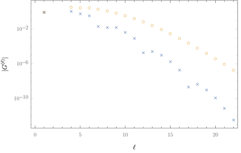
Figure 5: Logarithmic plot of the absolute value of the coefficients $G^{(\ell)}$ (81), for $\ell=1,\dots,22$. The $|G^{(\ell)}|$ quickly become very small suggesting good convergence of the series. Shown is the singlet (crosses) and ${27}$ exchange (circles).

Furthermore, we can establish that the anomalous dimension (76) has an infinite radius of convergence as a function of $x\equiv L\alpha_{s}/\pi$. To see this we write the resummed soft anomalous dimension as:

$${\bf\Gamma}_{{\mathrm{NLL}}}^{(-)}=i\pi\frac{\alpha_{s}}{\pi}\,G\left(\frac{\alpha_{s}}{\pi}L\right){\bf T}_{s{-}u}^{2}\,,$$ (80)

where the generating function for the expansion coefficients is defined by

$$G(x)=\sum_{\ell=1}^{\infty}x^{\ell-1}G^{(\ell)}\,.$$ (81)

It is convenient to further identify $G(x)$ as the Borel transform of some function

$$g(y)\equiv\int_{0}^{\infty}\!dx\,G(x)\,e^{-x/y}=\sum_{\ell=1}^{\infty}G^{(\ell)}y^{\ell}(\ell-1)!\,,$$ (82)

which upon using eq. (75), simply evaluates to

$$g(y)=\frac{y}{1-{\displaystyle\frac{C_{A}}{C_{A}-{\bf T}_{t}^{2}}\,R\left(y{(C_{A}-{\bf T}_{t}^{2})}/{2}\right)}}\,.$$ (83)

We may now recover the original $G(x)$ via the integral

$$G(x)=\frac{1}{2\pi i}\int_{w-i\infty}^{w+i\infty}d\eta\,g\left(\frac{1}{\eta}\right){\rm e}^{\eta x}\,,$$ (84)

where the integration contour runs parallel to the imaginary axis, to the right of all singularities of the integrand.

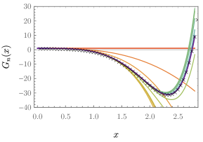
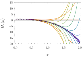
Figure 6: Partial sums $G_{n}(x)=\sum_{\ell=1}^{n}G^{(\ell)}x^{\ell-1}$ for $n=1,\dots,22$ (rainbow, red through violet) and numerical results for $G(x)$ (black crosses). The plot illustrates convergence in that increasing the order $n$ extends the range of $x$ for which the the partial sum matches the numerical result. The figure shows the singlet (left) as well as the ${27}$ exchange (right).

The function $g(y)$ in eq. (82) only has isolated poles away from the origin and has a finite radius of convergence: it is well-defined in a disc around the origin. It then follows that $G(x)$ has an infinite radius of convergence, hence this function — and the soft anomalous dimension ${\bf\Gamma}_{{\mathrm{NLL}}}^{(-)}$ in eq. (80) — is an entire function, free of any singularities for any finite $x=L\alpha_{s}/\pi$.

We stress that our use of the Borel transform is opposite to the usual application of Borel summation (which is ordinarily used to sum asymptotic series): the function $G(x)$, in which we are interested, is an entire function; we make use of its inverse Borel transform, $g(y)$, which has worse behaviour by having merely a finite radius of convergence. Nonetheless we find that numerically integrating eq. (84) is a particularly convenient way to evaluate the anomalous dimension. This numerical integration is compared to the partial sums

$$G_{n}(x)\equiv\sum_{\ell=1}^{n}G^{(\ell)}x^{\ell-1}$$ (85)

in figure 6, where we find good agreement for the given values of $x$. While it becomes challenging to efficiently compute the coefficients $G^{(\ell)}$ at high orders (here we only evaluated them for $\ell\leq 22$), we find the numerical integration of eq. (84) to be very stable, even for larger values of $x$. Thus, the remarkable convergence properties of $G(x)$ along with the Borel technique, presents us with the possibility of computing $\Gamma_{\rm NLL}^{(-)}$ for $x=L\alpha_{s}/{\pi}\,\gg\,1$, i.e. at asymptotically high energies. This is a rather unique situation in a perturbative setting — in other circumstances resummation techniques are limited to the region $x=L{\alpha_{s}}/{\pi}\,\lesssim\,1$.

Evaluating the integral (84) and plotting $G(x)$ for larger values of $x$ reveals oscillations with a constant period and an exponentially growing amplitude. Since this behaviour is difficult to capture graphically we instead show the logarithm of $|G(x)|$ weighted by the sign of $G(x)$ in figure 7.

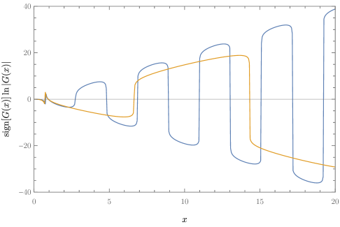
Figure 7: Numerical results for $\mathrm{sign}\left[G(x)\right]\ln\left|G(x)\right|$ for the singlet (blue) and ${27}$ exchange (orange). The “heartbeat” at small $x$ reflects the logarithmic divergence of $\ln\left|G(x)\right|$ where $G(x)$ changes its sign for the first time (similar divergences occur every oscillation but are not visible due to the finite resolution of the plot).

This observation suggests to approximate (84) by

$$G(x)\to c\,e^{ax}\cos\left(bx+d\right)\,,$$ (86)

for sufficiently large values of $x$. By means of eq. (82), this model is equivalent to

$$g\left(\frac{1}{\eta}\right)\to c\,{\rm Re}\left[\frac{e^{id}}{\eta-a-ib}\right]=\frac{c}{2}\left(\frac{e^{id}}{\eta-a-ib}+\frac{e^{-id}}{\eta-a+ib}\right)\,,$$ (87)

which is to be integrated as in (84) with a contour to the right of the poles.

	$a$	$b$	$c$	$d$
${1}$	1.97	1.52	0.25	0.48
${27}$	1.46	0.41	0.58	2.01

Table 1: Numerical results for $a,b,c$ and $d$, cf. eq. (86), for the singlet (${1}$) and ${27}$ representation.

We thus find that to capture the behaviour $G(x)$ at large $x$ it is sufficient to simply consider $g\left(\frac{1}{\eta}\right)$ as a pair of complex-conjugated poles at $\eta=a\pm ib$. Indeed, numerically extracting the rightmost poles of $g\left(\frac{1}{\eta}\right)$ of eq. (83) to identify the parameters $a$ and $b$ in eq. (87), and dividing the full, numerically-evaluated, $G(x)$ by $e^{ax}$ leaves us with almost pure cosine-like behaviour for any $x\gg 1$, as can be seen in figure 8. For reference, we quote our numerical results for $a,b,c$ and $d$ in table 1.

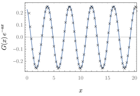
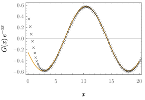
Figure 8: The approximation of eq. (86) for $G(x)$ for $x\gg 1$, divided by $e^{ax}$ (solid line) contrasted with numerical results (crosses). The coefficients $a$ and $b$ were extracted from the poles of $g(1/\eta)$ while $c$ and $d$ were fitted after dividing the full, numerically evaluated, $G(x)$ by $e^{ax}$. Already for moderate values of $x$ we observe excellent agreement. The singlet exchange is shown on the left and the ${27}$ is on the right.

4.4 Exponentiation check for higher-order infrared poles

As a final step we confirm the agreement between the BFKL prediction and the soft factorisation theorem. Thus far we have only used the single poles as predicted by the BFKL evolution to extract the NLL soft anomalous dimension ${\bf\Gamma}_{{\mathrm{NLL}}}^{(-)}$. As explained in section 4.1, higher-order poles of the amplitude are generated upon expansion of the path-ordered exponential in eq. (70). They have to match the BFKL computation and therefore provide an independent and non-trivial check of our results.

To see how this works, let us expand the BFKL result (71) to the first few orders, namely

$$\bar{\mathcal{M}}_{\rm NLL}^{(+)}\left(\frac{s}{-t}\right)=\sum_{\ell=1}^{\infty}\left(\frac{\alpha_{s}}{\pi}\right)^{\ell}\,L^{\ell-1}\,\bar{\mathcal{M}}_{\rm NLL}^{(+,\ell)}\,.$$ (88)

with

$$\bar{\mathcal{M}}_{\mathrm{NLL}}^{(+,1)} = i\pi\left[\frac{1}{2\epsilon}+O(\epsilon^{0})\right]{\bf T}_{s{-}u}^{2}\mathcal{M}^{(\rm tree)},$$ (89a)

$$\bar{\mathcal{M}}_{\mathrm{NLL}}^{(+,2)} = i\pi\frac{(C_{A}-{\bf T}_{t}^{2})}{2!}\left[\frac{1}{(2\epsilon)^{2}}+O(\epsilon^{0})\right]{\bf T}_{s{-}u}^{2}\mathcal{M}^{(\rm tree)},$$ (89b)

$$\bar{\mathcal{M}}_{\mathrm{NLL}}^{(+,3)} = i\pi\frac{(C_{A}-{\bf T}_{t}^{2})^{2}}{3!}\left[\frac{1}{(2\epsilon)^{3}}+O(\epsilon^{0})\right]{\bf T}_{s{-}u}^{2}\mathcal{M}^{(\rm tree)},$$ (89c)

$$\bar{\mathcal{M}}_{\mathrm{NLL}}^{(+,4)} = i\pi\frac{(C_{A}-{\bf T}_{t}^{2})^{3}}{4!}\left[\frac{1}{(2\epsilon)^{4}}-\frac{1}{2\epsilon}\frac{\zeta_{3}C_{A}}{4(C_{A}-{\bf T}_{t}^{2})}+O(\epsilon^{0})\right]{\bf T}_{s{-}u}^{2}\mathcal{M}^{(\rm tree)},$$ (89d)

$$\bar{\mathcal{M}}_{\mathrm{NLL}}^{(+,5)} = i\pi\frac{(C_{A}-{\bf T}_{t}^{2})^{4}}{5!}\bigg{[}\frac{1}{(2\epsilon)^{5}}-\frac{1}{(2\epsilon)^{2}}\frac{\zeta_{3}C_{A}}{4(C_{A}-{\bf T}_{t}^{2})}$$ (89e)

$$\hskip 85.35826pt-\,\frac{1}{2\epsilon}\frac{3\zeta_{4}C_{A}}{16(C_{A}-{\bf T}_{t}^{2})}+O(\epsilon^{0})\bigg{]}{\bf T}_{s{-}u}^{2}\mathcal{M}^{(\rm tree)}.$$

Let us begin with the leading pole. One can see a simple pattern in its $\ell$-th order coefficient, which is proportional to $(C_{A}-{\bf T}_{t}^{2})^{\ell-1}/(\ell!(2\epsilon)^{\ell})$. This should be compared with the prediction (70) from infrared exponentiation, which we reproduce here for convenience:

$$\bar{\mathcal{M}}_{\mathrm{NLL}}^{(+)}=-\int_{0}^{p}\frac{d\lambda}{\lambda}\exp\left\{\frac{1}{2\epsilon}\frac{\alpha_{s}(p)}{\pi}L(C_{A}-{\bf T}_{t}^{2})\left[1-\left(\frac{p^{2}}{\lambda^{2}}\right)^{\epsilon}\,\right]\right\}{\bf\Gamma}_{{\mathrm{NLL}}}^{(-)}\left(\alpha_{s}(\lambda)\right)\,\mathcal{M}^{(\rm tree)}+{\cal O}(\epsilon^{0}).$$ (90)

Substituting ${\bf\Gamma}_{{\mathrm{NLL}}}^{(-)}$ using eqs. (77) and (74), and taking into account that the running coupling $\alpha_{s}(\mu)=\alpha_{s}(p)\left(p^{2}/\mu^{2}\right)^{\epsilon}$, one gets

$$\bar{\mathcal{M}}_{\mathrm{NLL}}^{(+)}= -i\pi\sum_{k=1}^{\infty}G^{(k)}\left(\frac{\alpha_{s}(p)}{\pi}\right)^{k}\,L^{k-1}\int_{0}^{p}\frac{d\lambda}{\lambda}\left(\frac{p^{2}}{\lambda^{2}}\right)^{\epsilon k}$$

$$\qquad\times\exp\left\{\frac{1}{2\epsilon}\frac{\alpha_{s}(p)}{\pi}L(C_{A}-{\bf T}_{t}^{2})\left[1-\left(\frac{p^{2}}{\lambda^{2}}\right)^{\epsilon}\,\right]\right\}\,\,{\bf T}_{s{-}u}^{2}\,\mathcal{M}^{(\rm tree)}+{\cal O}(\epsilon^{0}).$$

For the leading pole it is clear that only the $G^{(1)}$ terms contribute, corresponding to the one-loop contribution to the soft anomalous dimension (63), and we then get:

$$\left[\bar{\mathcal{M}}_{\mathrm{NLL}}^{(+)}\right]_{\text{leading poles}} = -i\pi\,\frac{\alpha_{s}(p)}{\pi}\int_{0}^{p}\frac{d\lambda}{\lambda}\left(\frac{p^{2}}{\lambda^{2}}\right)^{\epsilon}$$ (92)

$$\quad\times\exp\left\{\frac{1}{2\epsilon}\frac{\alpha_{s}(p)}{\pi}L(C_{A}-{\bf T}_{t}^{2})\left[1-\left(\frac{p^{2}}{\lambda^{2}}\right)^{\epsilon}\,\right]\right\}{\bf T}_{s{-}u}^{2}\mathcal{M}^{(\rm tree)}$$

$$= -i\pi\left[\frac{\displaystyle\exp\left\{\frac{1}{2\epsilon}\frac{\alpha_{s}(p)}{\pi}L(C_{A}-{\bf T}_{t}^{2})\right\}-1}{L(C_{A}-{\bf T}_{t}^{2})}\right]{\bf T}_{s{-}u}^{2}\mathcal{M}^{(\rm tree)}\,.$$

Expanding in $\alpha_{s}$ this matches precisely the $1/(\ell!(2\epsilon)^{\ell})$ terms in eq. (89), with the correct prefactor. This exponentiation of leading poles had been verified previously in ref. Caron-Huot:2013fea . Moving on to the first subleading pole, the Regge prediction reveals a four-loop single pole in eq. (89d), as well as a five-loop double pole in eq. (89e) and so on, all proportional to $\zeta_{3}$. In general, expanding the BFKL result (71) to higher orders one finds a tower of such terms going like $1/(\ell!(2\epsilon)^{\ell-3})$. In the infrared exponentiation formula, these should be generated by a single parameter, the four-loop anomalous dimension, ${\bf\Gamma}^{(-,4)}_{\rm NLL}$, which is indeed proportional to $\zeta_{3}$ (see eq. (78)). It can be traced back to the leading-order term in the expansion of $R(\epsilon)$ in (49), contributing to $G^{(4)}$ in eq. (75). Similarly, a $k$-loop anomalous dimension ${\bf\Gamma}^{(-,k)}_{\rm NLL}$, in general, contributes in proportion to $G^{(k)}$. Indeed, integrating eq. (4.4) we find that

$$\bar{\mathcal{M}}_{\mathrm{NLL}}^{(+)}=\frac{i\pi}{2\epsilon}\sum_{k=1}^{\infty}\,G^{(k)}\,(k-1)!\sum_{\ell=k}^{\infty}\frac{1}{\ell!}\left(\frac{\alpha_{s}(p)}{\pi}\right)^{\ell}\,L^{\ell-1}\left(\frac{C_{A}-{\bf T}_{t}^{2}}{2\epsilon}\right)^{\ell-k}\,\,{\bf T}_{s{-}u}^{2}\,\mathcal{M}^{(\rm tree)}+{\cal O}(\epsilon^{0}).$$ (93)

Next we note that given $k$, all contributions with $\ell<k$ are either constant or vanish for $\epsilon\to 0$, and so in as far as the singularities are concerned the sum over $\ell$ can be performed over all positive integers, independently of $k$. This yields

$$\bar{\mathcal{M}}_{\mathrm{NLL}}^{(+)}=i\pi\,\sum_{k=1}^{\infty}\,\frac{G^{(k)}\,(k-1)!(2\epsilon)^{k-1}}{L\,\left({C_{A}-{\bf T}_{t}^{2}}\right)^{k}}\,\left[{\displaystyle\exp\left\{\frac{1}{2\epsilon}\frac{\alpha_{s}}{\pi}L(C_{A}-{\bf T}_{t}^{2})\right\}-1}\right]\,{\bf T}_{s{-}u}^{2}\,\mathcal{M}^{(\rm tree)}+{\cal O}(\epsilon^{0}).$$ (94)

This shows that infrared exponentiation works out if, and only if, all the poles in the NLL amplitude can be written as a function of $\epsilon$ only (i.e. independent of $\alpha_{s}$), times the quantity in the square bracket. With hindsight, infrared exponentiation thus explains the compact form of the BFKL result in eq. (71). Finally, it is straightforward to substitute in the definition of $G^{(k)}$ from eq. (75) and sum up the series over $k$, recovering the full result for the singularities of the amplitudes in eq. (71). This completes the proof that the BFKL result we obtained is consistent with infrared factorisation.

5 Conclusions

We considered the even signature component of two-to-two parton scattering amplitudes in the high-energy limit. This amplitude is dominated by the $t$-channel exchange of a state consisting of two Reggeized gluons, corresponding to the simplest example of a Regge cut in QCD. The amplitude can be evaluated in QCD perturbation theory by iteratively solving the BFKL equation. Each order in perturbation theory corresponds to one additional rung in the BFKL ladder, building up a tower of so-called next-to-leading logarithms, ${\cal O}(\alpha_{s}^{\ell}L^{\ell-1})$. Although the BFKL Hamiltonian has been diagonalised in many cases Lipatov:1985uk , the dimensionally-regulated Hamiltonian relevant for partonic amplitudes has remained more difficult to handle.

Our first observation was that the wavefunction describing the two Reggeized gluons remains finite through BFKL evolution for any number of rungs, while the corresponding amplitude develops infrared singularities due to the soft limit of the wavefunction. We further observed that the evolution of a state in which one of the two Reggeized gluons is much softer than the other, $k\ll p-k$, yields again a similar state. In other words, the soft approximation is consistent with BFKL evolution, and as a consequence, one can systematically solve the equation to any loop order within this approximation. We found that the soft approximation leads to a major simplification, where all integrals reduce to products of bubbles, and the wavefunction at any given order is simply a polynomial of that order in $\left(p^{2}/k^{2}\right)^{\epsilon}$. This eventually allowed us to determine the singularities of the amplitude in a closed form to any order, as given in eq. (50).

At the next step we contrasted the singularity structure we obtained though BFKL evolution with the known exponentiation properties of infrared singularities. As expected, we found that the two are consistent, and this provides a highly non-trivial check of the calculation. The leading singularity at each order, ${\cal O}(\alpha_{s}^{\ell}L^{\ell-1}/\epsilon^{\ell})$, is simply related to the one-loop soft anomalous dimension, and has a colour structure proportional to $(C_{A}-{\bf T}_{t}^{2})^{\ell-1}$. New singularities, with fewer powers of $1/\epsilon$ and different colour structures, appear starting from four loop. These correspond to new terms in the imaginary part of the soft anomalous dimension, eq. (78). We were thus able to determine the soft anomalous dimension at next-to-leading logarithmic accuracy in the high-energy limit to all orders. These results also provide a valuable input for determining the structure of long-distance singularities for general kinematics using a bootstrap approach, as done at the three-loop order in ref. Almelid:2017qju .

We point out that the $\ell$-loop coefficient of the soft anomalous dimension we computed is a linear combination of zeta values of weight $(\ell-1)$, which coincides with the maximal (transcendental) weight. This is not surprising given that these corrections are independent of the matter content nor the amount of supersymmetry of the theory, and are thus common for example to QCD and ${\cal N}=4$ super Yang-Mills. We further showed that these corrections to the soft anomalous dimension can be resummed, as in eq. (80), into an entire function of $x=L\alpha_{s}/\pi$. Remarkably, this gives us means to determine the asymptotic high-energy behaviour of this anomalous dimension, corresponding to $x\gg 1$, a regime which is usually inaccessible to perturbation theory. We find that at large $x$ the imaginary part of the anomalous dimension in the Regge limit, in any colour representation, becomes an oscillating function with an exponentially growing amplitude.

While our analysis in this paper was focused on infrared singularities, for which the soft approximation is sufficient, the formulation of the evolution in eq. (2.2) along with the observation that the wavefunction is finite, pave the way to determining the wavefunction beyond the soft approximation, thus evaluating the finite contributions to Regge-cut of two-to-two amplitudes. It would also be interesting to extend the present analysis to the next order, using the known next-to-leading order Hamiltonian; again we expect that a suitable wavefunction will remain finite to all orders, facilitating a direct determination of the infrared singularities.

Appendix A The even amplitude at NLL accuracy within the shockwave formalism

In this appendix we briefly review how eq. (13) can be derived within the shockwave formalism refs. Caron-Huot:2013fea ; Caron-Huot:2017fxr . Amplitudes in the high-energy limit are calculated as expectation values of null Wilson lines:

$$U(z_{\perp})=\mathcal{P}\exp\left[ig_{s}\int_{-\infty}^{+\infty}\,\mathrm{d}x^{+}\,A_{+}^{a}(x^{+},x^{-}{=\,}0,z_{\perp})\,T^{a}\right].$$ (95)

The latter follows the path of colliding partons from the projectile or target (with $x^{+}$ and $x^{-}$ interchanged), and are labelled by transverse coordinates $z_{\perp}$ (below we shall omit the subscript $\perp$ for lighter notation). The full transverse structure needs to be retained, because the high-energy limit is taken with fixed momentum transfer. Importantly, the number of Wilson lines cannot be held fixed, because the projectile and target contain an arbitrary number of virtual partons. However, in perturbation theory, the unitary matrices $U(z)$ are close to the identity and can therefore be usefully parametrised by a field $W$:

$$U(z)=e^{ig_{s}\,T^{a}W^{a}(z)}\,.$$ (96)

Physically, the colour-adjoint field $W^{a}$, which is propagating in the transverse space, is interpreted as source for a BFKL Reggeized gluon Caron-Huot:2013fea . At weak coupling a generic projectile is thus formed by a superposition of $W$ states. Up to NLL accuracy one needs to consider up to two Reggeons. In this approximation, a projectile, created with four-momentum $p_{1}$ and absorbed with $p_{4}$, is parameterised in momentum space as

$$|\psi_{i}\rangle \equiv \frac{Z_{i}^{-1}}{2p_{1}^{+}}a_{i}(p_{4})a^{\dagger}_{i}(p_{1})|0\rangle\,=\,|\psi_{i,1}\rangle+|\psi_{i,2}\rangle+\ldots\,,$$ (97)

where the ellipses stand for wavefunction components with three or more Reggeized gluons, which are not relevant at NLL accuracy. We next note that states with an even (odd) number of Reggeized gluons have an even (odd) signature, so

$$|\psi_{i,1}\rangle =|\psi_{i,1}^{(-)}\rangle=ig_{s}\,D_{i}^{(1)}(p){\bf T}_{i}^{a}\,W^{a}(p)$$ (98a)

$$|\psi_{i,2}\rangle =|\psi_{i,2}^{(+)}\rangle=-\frac{g_{s}^{2}}{2}{\bf T}_{i}^{a}{\bf T}_{i}^{b}\int\frac{\mathrm{d}^{2{-}2\epsilon}q}{(2\pi)^{2-2\epsilon}}\,\Omega^{(0)}(p,q)\,W^{a}(q)W^{b}(p{-}q),$$ (98b)

where $D_{i}^{(1)}(p)$ is an impact factor which parameterises the dependence of the coefficient on the (transverse) momentum transfer $p=p_{4}-p_{1}$ with $p^{2}=-t$. At the leading order, there is only one Wilson line $U(z)$ following the original parton, and the two-Reggeon wavefunction is obtained simply by expanding eq. (96), which gives, as in the main text:

$$\Omega^{(0)}(p,q)=1.$$ (99)

The null Wilson lines acquire energy dependence through rapidity divergences, which must be regulated, leading to the Balitsky-JIMWLK rapidity evolution equation:

$$\frac{d}{d\eta}\,|\psi_{i}\rangle=H\,|\psi_{i}\rangle\,.$$ (100)

The scattering amplitude can be obtained by computing the overlap between $\langle\psi_{j}|$ and $|\psi_{i}\rangle$, after evolving them to common rapidity, where the overlap is defined as the vacuum expectation value of left-moving and right-moving $W$-fields. In terms of the reduced amplitude defined in eq. (3) one has

$$\frac{i}{2s}\hat{\mathcal{M}}_{ij\to ij}=\langle\psi_{j}|e^{\hat{H}L}|\psi_{i}\rangle,\qquad\hat{H}\equiv H-{\bf T}_{t}^{2}\,\alpha_{g}(t).$$ (101)

Evolution at the desired accuracy is obtained by simply considering the Hamiltonian at leading order in $g_{s}^{2}$ in terms of $W$ fields, which, to this order, is diagonal:

$$\hat{H}\left(\begin{array}[]{c}W\\ WW\end{array}\right) \equiv \left(\begin{array}[]{ccc}\hat{H}_{1{\to}1}&0&\\ 0&\hat{H}_{2{\to}2}&\\ \end{array}\right)\left(\begin{array}[]{c}W\\ WW\end{array}\right)+{\cal O}(g_{s}^{4}).$$ (108)

Since the signature odd and even sectors are orthogonal and closed under the action of $\hat{H}$ (as a consequence of the signature symmetry), their contributions to the amplitude at NLL separate:

$$\frac{i}{2s}\hat{\mathcal{M}}^{\rm NLL}_{ij\to ij} = \frac{i}{2s}\left(\hat{\mathcal{M}}^{(-),\rm NLL}_{ij\to ij}+\hat{\mathcal{M}}^{(+),\rm NLL}_{ij\to ij}\right)$$ (109)

$$\equiv \langle\psi^{(-)}_{j,1}|e^{\hat{H}L}|\psi^{(-)}_{i,1}\rangle^{{\rm(NLO)}}+\langle\psi^{(+)}_{j,2}|e^{\hat{H}L}|\psi^{(+)}_{i,2}\rangle^{{\rm(LO)}},$$

where “LO” and “NLO” means that all ingredients are needed respectively to leading and next-to-leading nonvanishing order. In this paper we focus on the even amplitude, representing the exchange of a pair of Reggeons, corresponding to the second term in eq. (109). It is then convenient to compute the inner product in eq. (101) by first evolving the wavefunction:

$$e^{\hat{H}_{2\to 2}L}|\psi_{i,2}^{(+)}\rangle=-\frac{g_{s}^{2}}{2}{\bf T}_{i}^{a}{\bf T}_{i}^{b}\sum_{\ell=0}^{\infty}\frac{1}{\ell!}\left(\frac{\alpha_{s}B_{0}(\epsilon)L}{\pi}\right)^{\ell}\int\frac{\mathrm{d}^{2{-}2\epsilon}q}{(2\pi)^{2-2\epsilon}}\,\Omega^{(\ell)}(p,q)\,W^{a}(q)W^{b}(p{-}q)\,.$$ (110)

As displayed in eq. (15), the wavefunctions $\Omega^{(\ell)}$ may then be obtained iteratively by applying the Hamiltonian $\hat{H}_{2{\to}2}$. This Hamiltonian was discussed at length in terms of Wilson lines in ref. Caron-Huot:2017fxr , to which we refer for further details ($-H_{k\to k}$ is given in eq. (3.13) there; note the overall minus sign between our conventions). Acting with $\hat{H}_{2{\to}2}$ on the states in eq. (110), reproduces precisely the leading order BFKL Hamiltonian recorded in the main text. Finally, computing the overlap with the target state $\langle\psi^{(+)}_{j,2}|$ produces the integral which closes the ladder in eq. (13).

Appendix B Proof of the all-order amplitude

In this appendix we show that the singular terms in eq. (47) are equal to those in eq. (45). We start by noticing that the statement is equivalent to

$$\sum_{n=1}^{\ell}(-1)^{n+1}\,\binom{\ell}{n}\prod_{m=0}^{n-2}\bigg{[}1-\hat{B}_{m}(\epsilon)\frac{2C_{A}-{\bf T}_{t}^{2}}{C_{A}-{\bf T}_{t}^{2}}\bigg{]}-\left(1-\hat{B}_{-1}(\epsilon)\frac{2C_{A}-{\bf T}_{t}^{2}}{C_{A}-{\bf T}_{t}^{2}}\right)^{-1}={\cal O}(\epsilon^{\ell}).$$ (111)

Multiplying both sides of this equality by $\left(1-\hat{B}_{-1}(\epsilon)\frac{2C_{A}-{\bf T}_{t}^{2}}{C_{A}-{\bf T}_{t}^{2}}\right)=1+{\cal O}(\epsilon^{3})$ we get

$$\sum_{n=1}^{\ell}(-1)^{n+1}\,\binom{\ell}{n}\prod_{m=0}^{n-2}\bigg{[}1-\hat{B}_{m}(\epsilon)\frac{2C_{A}-{\bf T}_{t}^{2}}{C_{A}-{\bf T}_{t}^{2}}\bigg{]}\left(1-\hat{B}_{-1}(\epsilon)\frac{2C_{A}-{\bf T}_{t}^{2}}{C_{A}-{\bf T}_{t}^{2}}\right)-1={\cal O}(\epsilon^{\ell}).$$ (112)

The additional factor multiplying the sum on the l.h.s. can be incorporated into the product. Similarly, the $-1$ on the l.h.s. can be included in the sum. We obtain

$$\sum_{n=0}^{\ell}(-1)^{n+1}\,\binom{\ell}{n}\prod_{m=-1}^{n-2}\bigg{[}1-\hat{B}_{m}(\epsilon)\frac{2C_{A}-{\bf T}_{t}^{2}}{C_{A}-{\bf T}_{t}^{2}}\bigg{]}={\cal O}(\epsilon^{\ell}).$$ (113)

At this point, we realise that the structure of the sum and product is strikingly similar to that appearing in the target-averaged wavefunction in eq. (43). In that case, finitness of the $\ell$-loop wavefunction implies

$$\sum_{n=0}^{\ell}(-1)^{n}n^{q}\binom{\ell}{n}\prod_{m=0}^{n-1}\left[1-\hat{B}_{m}(\epsilon)\frac{2C_{A}-{\bf T}_{t}^{2}}{C_{A}-{\bf T}_{t}^{2}}\right]={\cal O}\left(\epsilon^{\ell-q}\right)\quad\text{with}\quad q=0,1,2,\dots$$ (114)

which is obtained by expanding $(p^{2}/k^{2})^{n\epsilon}$ around small $\epsilon$ inside the sum. Next, we bring the product in eq. (113) to the same form as in eq. (114), obtaining

$$\sum_{n=0}^{\ell}(-1)^{n+1}\,\binom{\ell}{n}\left(1-\hat{B}_{-1}(\epsilon)\frac{2C_{A}-{\bf T}_{t}^{2}}{C_{A}-{\bf T}_{t}^{2}}\right)\left(1-\hat{B}_{n-1}(\epsilon)\frac{2C_{A}-{\bf T}_{t}^{2}}{C_{A}-{\bf T}_{t}^{2}}\right)^{-1}$$ (115)

$$\times\,\prod_{m=0}^{n-1}\bigg{[}1-\hat{B}_{m}(\epsilon)\frac{2C_{A}-{\bf T}_{t}^{2}}{C_{A}-{\bf T}_{t}^{2}}\bigg{]}={\cal O}(\epsilon^{\ell}).$$

The extracted factor

$$\left(1-\hat{B}_{-1}(\epsilon)\frac{2C_{A}-{\bf T}_{t}^{2}}{C_{A}-{\bf T}_{t}^{2}}\right)\left(1-\hat{B}_{n-1}(\epsilon)\frac{2C_{A}-{\bf T}_{t}^{2}}{C_{A}-{\bf T}_{t}^{2}}\right)^{-1}\\ =1+\frac{2C_{A}-{\bf T}_{t}^{2}}{C_{A}-{\bf T}_{t}^{2}}\left[2\epsilon(n\epsilon)^{2}\zeta_{3}+3\epsilon^{2}(n\epsilon)^{2}\zeta_{4}+\left(4\epsilon^{3}(n\epsilon)^{2}+2\epsilon(n\epsilon)^{4}\right)\zeta_{5}\right]+{\cal O}(\epsilon^{6})$$ (116)

is a function of $\epsilon$ and $\delta\equiv n\epsilon$, cf. eqs. (39) and (41), which are both small. In other words, the (double) expansion of eq. (116) in $\epsilon$ and $\delta$ around 0 contains only terms for which the power of $\epsilon$ is equal or greater than the power of $n$. This, then, together with eq. (114), proves eq. (113) and thus the conjectured amplitude (47).

References

- (1) E. A. Kuraev, L. N. Lipatov and V. S. Fadin, The Pomeranchuk Singularity in Nonabelian Gauge Theories, Sov. Phys. JETP 45 (1977) 199–204.
- (2) I. I. Balitsky and L. N. Lipatov, The Pomeranchuk Singularity in Quantum Chromodynamics, Sov. J. Nucl. Phys. 28 (1978) 822–829.
- (3) L. N. Lipatov, The Bare Pomeron in Quantum Chromodynamics, Sov. Phys. JETP 63 (1986) 904–912.
- (4) A. H. Mueller, Soft gluons in the infinite momentum wave function and the BFKL pomeron, Nucl. Phys. B415 (1994) 373–385.
- (5) A. H. Mueller and B. Patel, Single and double BFKL pomeron exchange and a dipole picture of high-energy hard processes, Nucl. Phys. B425 (1994) 471–488, [hep-ph/9403256].
- (6) R. C. Brower, J. Polchinski, M. J. Strassler and C.-I. Tan, The Pomeron and gauge/string duality, JHEP 12 (2007) 005, [hep-th/0603115].
- (7) I. Moult, M. P. Solon, I. W. Stewart and G. Vita, Fermionic Glauber Operators and Quark Reggeization, 1709.09174.
- (8) I. Balitsky, Operator expansion for high-energy scattering, Nucl. Phys. B463 (1996) 99–160, [hep-ph/9509348].
- (9) I. Balitsky, Factorization for high-energy scattering, Phys. Rev. Lett. 81 (1998) 2024–2027, [hep-ph/9807434].
- (10) Y. V. Kovchegov, Small x F(2) structure function of a nucleus including multiple pomeron exchanges, Phys. Rev. D60 (1999) 034008, [hep-ph/9901281].
- (11) J. Jalilian-Marian, A. Kovner, L. D. McLerran and H. Weigert, The Intrinsic glue distribution at very small x, Phys. Rev. D55 (1997) 5414–5428, [hep-ph/9606337].
- (12) J. Jalilian-Marian, A. Kovner, A. Leonidov and H. Weigert, The Wilson renormalization group for low x physics: Towards the high density regime, Phys. Rev. D59 (1998) 014014, [hep-ph/9706377].
- (13) E. Iancu, A. Leonidov and L. D. McLerran, The Renormalization group equation for the color glass condensate, Phys. Lett. B510 (2001) 133–144, [hep-ph/0102009].
- (14) M. G. Sotiropoulos and G. F. Sterman, Color exchange in near forward hard elastic scattering, Nucl. Phys. B419 (1994) 59–76, [hep-ph/9310279].
- (15) G. P. Korchemsky, On Near forward high-energy scattering in QCD, Phys. Lett. B325 (1994) 459–466, [hep-ph/9311294].
- (16) I. A. Korchemskaya and G. P. Korchemsky, Evolution equation for gluon Regge trajectory, Phys. Lett. B387 (1996) 346–354, [hep-ph/9607229].
- (17) I. A. Korchemskaya and G. P. Korchemsky, High-energy scattering in QCD and cross singularities of Wilson loops, Nucl. Phys. B437 (1995) 127–162, [hep-ph/9409446].
- (18) V. Del Duca and E. W. N. Glover, The High-energy limit of QCD at two loops, JHEP 10 (2001) 035, [hep-ph/0109028].
- (19) V. Del Duca, G. Falcioni, L. Magnea and L. Vernazza, High-energy QCD amplitudes at two loops and beyond, Phys. Lett. B732 (2014) 233–240, [1311.0304].
- (20) V. Del Duca, G. Falcioni, L. Magnea and L. Vernazza, Analyzing high-energy factorization beyond next-to-leading logarithmic accuracy, JHEP 02 (2015) 029, [1409.8330].
- (21) V. Del Duca, C. Duhr, E. Gardi, L. Magnea and C. D. White, An infrared approach to Reggeization, Phys. Rev. D85 (2012) 071104, [1108.5947].
- (22) V. Del Duca, C. Duhr, E. Gardi, L. Magnea and C. D. White, The Infrared structure of gauge theory amplitudes in the high-energy limit, JHEP 12 (2011) 021, [1109.3581].
- (23) S. Caron-Huot, When does the gluon reggeize?, JHEP 05 (2015) 093, [1309.6521].
- (24) S. Caron-Huot, E. Gardi and L. Vernazza, Two-parton scattering in the high-energy limit, JHEP 06 (2017) 016, [1701.05241].
- (25) P. D. B. Collins, An Introduction to Regge Theory and High-Energy Physics. Cambridge Monographs on Mathematical Physics. Cambridge Univ. Press, Cambridge, UK, 2009.
- (26) O. Almelid, C. Duhr and E. Gardi, Three-loop corrections to the soft anomalous dimension in multileg scattering, Phys. Rev. Lett. 117 (2016) 172002, [1507.00047].
- (27) E. Gardi, O. Almelid and C. Duhr, Long-distance singularities in multi-leg scattering amplitudes, PoS LL2016 (2016) 058, [1606.05697].
- (28) S. M. Aybat, L. J. Dixon and G. F. Sterman, The Two-loop soft anomalous dimension matrix and resummation at next-to-next-to leading pole, Phys. Rev. D74 (2006) 074004, [hep-ph/0607309].
- (29) E. Gardi and L. Magnea, Factorization constraints for soft anomalous dimensions in QCD scattering amplitudes, JHEP 03 (2009) 079, [0901.1091].
- (30) T. Becher and M. Neubert, Infrared singularities of scattering amplitudes in perturbative QCD, Phys. Rev. Lett. 102 (2009) 162001, [0901.0722].
- (31) T. Becher and M. Neubert, On the Structure of Infrared Singularities of Gauge-Theory Amplitudes, JHEP 06 (2009) 081, [0903.1126].
- (32) O. Almelid, C. Duhr, E. Gardi, A. McLeod and C. D. White, Bootstrapping the QCD soft anomalous dimension, JHEP 09 (2017) 073, [1706.10162].
- (33) Yu. L. Dokshitzer and G. Marchesini, Soft gluons at large angles in hadron collisions, JHEP 01 (2006) 007, [hep-ph/0509078].
- (34) S. Catani, The Singular behavior of QCD amplitudes at two loop order, Phys. Lett. B427 (1998) 161–171, [hep-ph/9802439].
- (35) E. Gardi and L. Magnea, Infrared singularities in QCD amplitudes, Nuovo Cim. C32N5-6 (2009) 137–157, [0908.3273].
- (36) L. J. Dixon, E. Gardi and L. Magnea, On soft singularities at three loops and beyond, JHEP 02 (2010) 081, [0910.3653].
- (37) V. Ahrens, M. Neubert and L. Vernazza, Structure of Infrared Singularities of Gauge-Theory Amplitudes at Three and Four Loops, JHEP 09 (2012) 138, [1208.4847].
- (38) G. P. Korchemsky and A. V. Radyushkin, Loop Space Formalism and Renormalization Group for the Infrared Asymptotics of QCD, Phys. Lett. B171 (1986) 459–467.
- (39) G. P. Korchemsky and A. V. Radyushkin, Infrared asymptotics of perturbative QCD: renormalisation properties of the Wilson loops in higher orders of perturbation theory, Sov. J. Nucl. Phys. 44 (1986) 877.
- (40) G. P. Korchemsky and A. V. Radyushkin, Renormalization of the Wilson Loops Beyond the Leading Order, Nucl. Phys. B283 (1987) 342–364.