Enhanced Rates of Fast Radio Bursts from Galaxy Clusters

Abstract

Fast Radio Bursts (FRBs) have so far been detected serendipitously across the sky. We consider the possible enhancement in the FRB rate in the direction of galaxy clusters, and compare the predicted rate from a large sample of galaxy clusters to the expected cosmological mean rate. We show that clusters offer better prospects for a blind survey if the faint end of the FRB luminosity function is steep. We find that for a telescope with a beam of $\sim 1$ deg², the best targets would be either nearby clusters such as Virgo or clusters at intermediate cosmological distances of few hundred Mpc, which offer maximal number of galaxies per beam. We identify several galaxy clusters which have a significant excess FRB yield compared to the cosmic mean. The two most promising candidates are the Virgo cluster containing 1598 galaxies and located 16.5 Mpc away and S34 cluster which contains 3175 galaxies and is located at a distance of 486 Mpc.

1. Introduction

Fast radio bursts (FRBs) are rapid transients detected in the $\sim 0.7-1.8$ GHz frequency range and characterized by a few millisecond duration. Since the discovery of the first FRB in 2007 (Lorimer et al., 2007), 23 additional bursts were observed by several radio telescopes in different regions of the sky (Keane et al., 2011; Thornton et al., 2013; Burke-Spolaor & Bannister, 2014; Petroff et al., 2015; Ravi et al., 2015; Champion et al., 2016; Keane et al., 2016; Ravi et al., 2016; Petroff et al., 2017; Masui et al., 2015; Caleb et al., 2017; Bannister et al., 2017, see the online FRB catalog for more details on the detected events). The repetitive nature of one of the bursts, FRB121102, allowed its localization to a few arcminutes and the identification of the host galaxy at a redshift 0.2 (Chatterjee et al., 2017; Tendulkar et al., 2017). This discovery demonstrated that at least some FRBs are of cosmological origin.

FRBs located at large cosmological distances can be used as probes of both their host environment and the intergalactic medium along the line of sight. As an FRB propagates through the ionized intergalactic medium, its pulse is dispersed in a frequency-dependent manner. The dispersion measure (DM) is proportional to the integrated electron column along the line of sight in (units of pc cm^-−3) which can be directly related to the redshift of the source after the contributions of the host galaxy and of the Milky Way are subtracted out. If FRBs exist prior to the Epoch of Reionization, their DM can constrain the reionization history and measure the total optical depth with sub-percent accuracy (Fialkov & Loeb, 2016). Surveying the population of FRBs could, therefore, not only reveal their origin, but also improve our understanding of cosmic history.

Up to now, FRBs have been discovered serendipitously across the sky. However, observational effort is on the way to perform more focused FRB searches and pin down the nature of these sources. Future surveys include the Canadian Hydrogen Intensity Mapping Experiment (CHIME), which is expected to have 125 mJy flux limit in the $400-800$ MHz frequency range and a large collecting area (Newburgh et al., 2014; Rajwade & Lorimer, 2017), as well as targeted searches with the Green Bank Telescope (GBT) at 1.4 GHz. Future facilities such as the Square Kilometer Array (SKA) are predicted to detect many more of these events (Fialkov & Loeb, 2016, 2017).

The origin of FRBs is still a mystery and it is unclear what are the properties, progenitors and host galaxies of these transients (e.g., Houde et al., 2017; Metzger et al., 2017; Beloborodov, 2017; Cordes & Wasserman, 2016). Recently, Macquart & Ekers (2017) examined the population of FRBs and found that current data is weakly inconsistent with flat luminosity function and implies only a very weak constraint on the slope of the integrated number counts to be $<-−1.3$ with the most likely value being $-−2.6^{+0.4}_{-0.6}$.

In this paper we study the possible enhancement in the FRB rate through observations of dense environments such as rich galaxy clusters. To bracket the large uncertainty we consider different scenarios varying the nature of the progenitors and the luminosity function of FRB. The paper is organized as follows. In Section 2 we outline our model assuming that the population of FRBs is of cosmological origin. In Section 3 we consider the Virgo cluster as a prototype and estimate the rate and distribution of FRBs from the cluster center using a public catalog of galaxies (Kim et al., 2014). In Section 4 we apply the formalism to a large sample of clusters from public galaxy cluster catalogs of the Sloan Digital Sky Survey (SDSS Einasto et al., 2007; Liivamagi et al., 2012). We summarize our conclusions in Section 5.

2. Cosmological population of FRBs

The expected rate and spatial distribution of FRBs strongly depends on their origin. Even under the assumption of a cosmological origin, there is a large variety of possible progenitors of FRBs. Since the host galaxy population is not yet constrained by observations, we consider two different scenarios in our modeling, assuming that FRBs are produced by either old or young stars. In addition, we consider two different shapes of the FRB luminosity function and vary the luminosity of the faintest events. Our cosmological models are summarized in the first Column of Table 1. We assume no repetitions of FRBs in our calculation.

Model	$R_{\rm int}/\dot{N}_{4}$	$N^{\rm Cosm}_{{\rm all}~{}z,~{}1~{}{\rm deg}^{2}}/\dot{N}_{4}$	$N^{\rm Virgo}_{{\rm max},~{}1~{}{\rm deg}^{2}}/\dot{N}_{4}$	$N^{\rm Cosm}_{V_{\rm Virgo}}/\dot{N}_{4}$	$N^{\rm Virgo}_{V_{\rm Virgo}}/\dot{N}_{4}$
#1 M*, SC	314 M${}_{\odot}^{-1}$	1.6	0.099	$8.4\times 10^{-4}$	1.58
#2 M*, Sch${}^{\alpha=-2}_{inst}$	$8.9\times 10^{11}$ M${}_{\odot}^{-1}$	0.92	$6.5\times 10^{3}$	55.3	$1.04\times 10^{5}$
#3 M*, Sch${}^{\alpha=-2}_{obs}$	$6.0\times 10^{3}$ M${}_{\odot}^{-1}$	1.06	1.89	0.016	30.2
#4 SFR, SC	0.0012 yr-1	0.45	0.0525	$1.9\times 10^{-4}$	0.899
#5 SFR, Sch${}^{\alpha=-2}_{inst}$	$8.2\times 10^{6}$ yr-1	0.58	$8.6\times 10^{3}$	1.1	$1.5\times 10^{5}$
#6 SFR, Sch${}^{\alpha=-2}_{obs}$	0.048 yr-1	0.59	2.18	0.008	37.4

Table 1Summary of model predictions assuming a flat spectrum for FRBs and $S_{\rm lim}=$ 30 Jy. Column 1: model description, low-luminosity cutoff $L_{\rm min}$ is determined either by the instrument ($S_{\rm min}^{\rm inst}$) or by the observed FRB with the lowest intrinsic luminosity ($S_{\rm min}^{\rm obs}$); Column 2: the inferred FRB normalization per galaxy in units of $\dot{N}_{4}=\dot{N}_{\rm obs}/10^{4}$ where $\dot{N}_{\rm obs}\sim 10^{3}-10^{5}$ sky^-1 day^-1 is the observed rate; Column 3: average number of FRBs per 1 deg² yr^-1 integrated over the entire redshift range out to $z=10$ in units of $\dot{N}_{4}$; Column 4: peak FRB rate from Virgo per year in a 1 deg² beam in units of $\dot{N}_{4}$. Column 5: average number of FRBs per year in units of $\dot{N}_{4}$ from a random patch of the sky of the virial volume of Virgo ($4\pi R_{\rm vir}^{3}/3$, $R_{\rm vir}=1.72$) located at the redshift of Virgo $z=0.002$ (16.5 Mpc). Column 6: same number as in Column 5 but for the real distribution of galaxies in Virgo extracted from the online Virgo catalog (Kim et al., 2014).

In the first scenario FRBs are produced in star forming regions and trace the population of newly born (massive) stars. In this case, the rate of FRBs in each individual galaxy would be proportional to its star formation rate (SFR), $\dot{N}_{1}=R^{\rm int}_{\rm SFR}\times$SFR, where SFR is in units of M_⊙ yr^-1. $R^{\rm int}_{\rm SFR}$ is the normalization constant (in units of M${}_{\odot}^{-1}$, yielding the FRB rate in units of yr^-1). When considering a cosmological population of galaxies, we adopt the SFR derived by Behroozi et al. (2013). This model, based on observations across a wide range of stellar masses $M_{*}\sim 10^{7}-10^{12}$ M_⊙ and redshifts ($z=0-8$), provides the star formation rate as a function of dark matter halo masses $\left(M_{h}\right)$ and redshift.

The second scenario is that FRBs are produced by old progenitors. In this case, FRB rate (in units of yr^-1) scales as the total stellar mass, $M_{*}$, and is $\dot{N}_{1}=R^{\rm int}_{*}M_{*}/M_{\rm Virgo}$ with $R^{\rm int}_{*}$ being the normalization constant in units of yr^-1. In the context of clusters, we normalize the total stellar mass by the mass of the Virgo galaxy cluster, $M_{\rm Virgo}=1.2\times 10^{15}$ M_⊙. Stellar mass can be related to the host halo mass (e.g., Mashian et al., 2016) via the star formation efficiency which we also adopt from the work by Behroozi et al. (2013).

The FRB rate from a large cosmological volume $V$ is obtained by integrating over the entire population of star forming halos in it. The number of halos in each mass bin $\Delta M_{h}$ is $\Delta M_{h}dn/dM_{h}$ per comoving Mpc³, and can be derived from the Press–Schechter formalism (Press & Schechter, 1974), or more accurately from the Sheth–Tormen mass function (Sheth & Tormen, 1999) which was calibrated against numerical simulations. The rate of FRBs in units of sky^-1 yr^-1 observed at redshift $z=0$ from the entire cosmological galaxy population is thus

$$\dot{N}_{\rm FRB}=\int_{V}dV\int_{M_{h}}dM_{h}\frac{dn}{dM_{h}}\frac{\dot{N}_{1}}{(1+z)},$$ (1)

where $V$ is the comoving volume and we integrate over host halo mass. The redshift factor $(1+z)^{-1}$ accounts for cosmological time dilation.

To bracket the large uncertainty in the FRB luminosity functions we consider two different scenarios:
(i) FRBs are standard candles (SC) of the same peak luminosity $\nu L_{\nu}=2.8\times 10^{43}$ erg s^-1, which corresponds to the mean intrinsic luminosity of the observed FRBs. To derive this value we used the online FRB catalog. For each event, the intrinsic isotropic luminosity can be derived based of the reported peak flux $S_{peak}$ and the redshift estimated from the DM, with $L_{\nu}=4\pi D_{L}^{2}S_{\rm peak}(1+z)^{-1}$ where $D_{L}$ is the luminosity distance. We then multiply by $\nu=1$ GHz, the typical frequency at which FRBs are observed, to get $\nu L_{\nu}$ and calculate the mean value across the ensemble of the observed FRBs.
(ii) FRBs have a Schechter (Sch) luminosity function

$$\frac{dn}{dL_{\nu}}=\left(\frac{L_{\nu}}{L_{\nu*}}\right)^{-\alpha}\exp\left[-\frac{L_{\nu}}{L_{\nu*}}\right]$$

with $\nu L_{\nu*}=2.8\times 10^{43}$ erg s^-1 and the faint-end slope of $\alpha=-2$. This is the steepest slope for which the luminosity density of a cosmological population converges, and this slope is broadly consistent with current observational constraints (Macquart & Ekers, 2017).

An additional free parameter in the case of a Schechter luminosity function is the low luminosity cutoff, $L_{\nu,min}$, the lowest luminosity of FRBs. In popular theoretical models FRBs, are launched by young magnetars (Cordes & Wasserman, 2016; Beloborodov, 2017; Metzger et al., 2017); however, FRBs appear to be $\mathcal{O}\left(10^{10}\right)$ times brighter than the typical magnetars found in our vicinity (Maoz & Loeb, 2017). To allow for the wide range of possibilities we, therefore, consider two cases: (1) $L_{\rm min}$ is set to be the luminosity of the intrinsically faintest observed FRB, $L_{\nu,{\rm min}}=L_{\nu,{\rm min}}^{\rm obs}$, namely FRB010621 with $\nu L_{\nu}^{\rm peak}=5.1\times 10^{41}$ erg s^-1; (2) FRBs can be as faint as the galactic magnetars resulting in $L_{\nu,{\rm min}}=\left(L_{\nu,*}/10^{10}\right)$. In the latter case, it is the telescope sensitivity, $S_{\rm lim}$, which sets the lower limit on the flux of observed events.

The number of events detected by a given radio observatory depends on several factors. To be detectable, the flux of a redshifted burst should be above the sensitivity limit of the telescope, $S_{\rm lim}$, and, if the burst has a limited frequency band, it should fall within the sensitivity band of the telescope. Here, for simplicity, we assume a flat spectrum (i.e., flux being independent of observing frequency) and set the flux limit to $S_{\rm lim}=30$ Jy having in mind a wide field survey with a small radio telescope. One such experiment is currently in operation at the Green Bank Observatory and makes use of the 20 m antenna there to carry out searches for FRBs at 1.4 GHz (Golpayegani et al. in prep.). This system has $S_{\rm lim}=30$ Jy over a 1 deg² field of view.

To calibrate each cosmological model we compare the expected rate of FRBs from Eq. (1) to the observational constraint which yields $\dot{N}_{\rm obs}\sim 10^{3}-10^{5}$ FRBs sky^-1 day^-1 at $z<1$ and $S_{\rm lim}\geq 1$ Jy (e.g., Keane & Petroff, 2015; Nicholl et al., 2017; Law et al., 2017). The results for normalization in each case are shown in the second Column of Table 1, in units of $\dot{N}_{4}$ sky^-1 yr^-1, where $\dot{N}_{4}\equiv 10^{-4}\dot{N}_{\rm obs}$ and $\dot{N}_{\rm obs}$ is in units of $\rm{sky}^{-1}~{}\rm{day}^{-1}$. For the Schechter luminosity function with the low-luminosity cutoff being set by telescope sensitivity, there is no way to constrain the faint end of the population and many faint events can occur per galaxy. This explains the very high relative normalization and expected number counts from nearby clustered environments. Using our cosmological model and integrating over the entire redshift range out to $z=10$, we then compute the mean FRB rate expected from a solid angle of 1 deg² per year (Column 3 of Table 1) and observed by a telescope with $S_{\rm lim}=30$ Jy.

3. FRB Rate from the Virgo Cluster

Next, we explore the expected FRB rates from clustered environments and compare the predicted numbers to the cosmological mean derived above. As a proof of concept we focus on the nearby Virgo cluster. Using the online Virgo catalog (Kim et al., 2014) which lists cluster members and the luminosity of each galaxy in every SDSS band, we infer stellar masses and SFRs for each galaxy in the cluster and estimate the expected number of FRBs for the actual distribution of galaxies.

3.1. Stellar mass

Stellar masses can be derived for individual Virgo galaxies by using standard mass-luminosity relations. To derive total stellar mass we follow Bernardi et al. (2010). The mass-luminosity relation at redshift $z=0$ is given as a function of $(g-r)_{0}$ colors

$$\log_{10}\left(M_{*}/L_{r}\right)=1.097\left(g-r\right)_{0}+z_{p},$$

where $z_{p}$ depends on the initial mass function (IMF) and, following Bernardi et al. (2010), we set $z_{p}=-0.406$ (Chabrier IMF, Bernardi et al., 2010). The magnitude in the r-band (which provides the luminosity in the r-band, $L_{r}$) is calculated as $M_{r}=r_{AB}-5\left[\log(D_{\rm Virgo,~{}pc})-1\right]$. Stellar mass is then calculated from

$$\log_{10}M_{*}=1.097(g-r)_{0}-0.406-0.4(M_{r}-4.67)$$ (2)

and $(g-r)_{0}$ is extracted from the catalog.

3.2. Star Formation Rate

The SFR in star forming galaxies follows a well known characteristic relation with the stellar mass (e.g., Brinchmann et al., 2004) referred to as the main sequence of galaxies (e.g., Noeske et al., 2007) and parametrized as

$$\log_{10}(\rm{SFR})=a\log_{10}\left(M_{*}\right)+b.$$ (3)

To compute SFR for the Virgo galaxies, we apply the aperture-free SFR-M_∗ relation (Duarte Puertas et al., 2017) and use $M_{*}$ obtained in the Section 3.1 above. Duarte Puertas et al. (2017) derived the total SFR for $\sim$210,000 SDSS star-forming galaxies using an empirically based aperture correction of the measured H$\alpha$ fluxes which have been extinction-corrected. The SFR$-M_{*}$ relation has been obtained in six redshift bins, over the redshift range $0.005<z<0.22$ with $a=0.935$ and $b=-9.208$. We use these values of $a$ and $b$ in Eq. (3) to estimate the SFR of each galaxy in the Virgo cluster.

3.3. Expected FRB Rate

We use the derived $M_{*}$ and SFR, along with the number of galaxies extracted from the catalog, to calculate the expected rate of FRBs from the entire Virgo cluster. As we see from Table 1, the largest effect on the observed FRB rate from nearby sources (e.g., galaxies in Virgo) is that of the luminosity function, while the nature of the hosts (young versus old stars) has a stronger effect on the cosmological background rate. With the real spacial distribution of galaxies in Virgo (Kim et al., 2014), we infer the expected rate of FRBs per each beam of 1 deg² and show the resulting sky distribution in Figure 1 with the assumptions of model #6 from Table 1. The few bright regions on this map indicate the optimal spots to target in a future search for FRBs in Virgo.

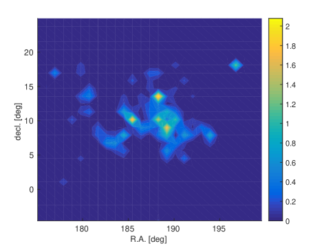
Figure 1.— FRB rates from Virgo in deg^-2 yr^-1 assuming $\dot{N}_{\rm obs}=10^{4}$ sky^-1 day^-1 for the model #6 from Table 1. Coordinates of the region with the highest FRB rate within Virgo are R.A. = 188.28 and Dec. = 13.58.

For a wide-band spectrum of FRBs (similar to the flat spectrum assumed here) observing the clustered environment is beneficial only if the faint-end slope of the luminosity function is steep (such as suggested by current observations Macquart & Ekers, 2017). This can be seen by comparing Column 3 to Column 4 in Table 1 for the rates within a 1 deg². If the population of faint FRBs is significant, the rate from clusters will exceed the cosmological mean by factor of a few in models #3 and 6 and by few orders of magnitude in models #2 and 5. On the other hand, if FRBs are standard candles (models #1 and 4, mildly inconsistent with observations Macquart & Ekers, 2017), dense nearby clusters such as Virgo would only contribute $\sim 10\%$ of the total observed FRB rate. Thus, clusters offer a new way to test the faint end of the luminosity function of FRBs.

Spectrum of FRBs also plays a role. If FRBs are narrow-band (e.g., similar to FRB121102 Law et al., 2017), only FRBs from a bounded redshift range fall within the telescope band. In this case, the FRB rate from clustered environments might exceed the mean cosmological rate even if they are standard candles. We demonstrate this by comparing the FRB rates for the virial volume of Virgo inhabited by a mean cosmological population of galaxies (Column 5) to the rate generated by a real distribution of galaxies in the cluster. For the scenarios under consideration, the total FRB yield is more than $1000$ times larger from the cluster than from a random field of the same virial size.

4. FRB from Galaxy Clusters

Next, we apply the formalism outlined above to a larger sample of galaxy clusters located at comoving distances out to $\sim 800$ Mpc, using two different catalogs, namely the 2dF catalog (Einasto et al., 2007) and the SDSS-DR7 sample (Liivamagi et al., 2012). The catalogs provide information on the number of galaxies within virial radius of each cluster. Assuming that the number of FRBs scales as the number of galaxies, we estimate the FRB rate per each individual cluster by simply re-scaling the number counts from Virgo. The expected intrinsic rate from a cluster is thus $\dot{N}_{\rm FRB}^{\rm cl}=\dot{N}_{\rm FRB}^{\rm Virgo}\times N_{\rm gal}^{\rm cl}/N_{\rm gal}^{\rm Virgo}$. FRB rate per cluster and the average FRB rate per beam for each cluster are shown in Figure 2 for each one of the considered models. To calculate the FRB rate per beam we divide the total FRB rate from the virial volume of each cluster by max$\left[A_{\rm eff},1~{}\rm{deg}^{2}\right]$ with $A_{\rm eff}$ being the effective area of the cluster. The rate from clusters is compared to the cosmological mean background (horizontal lines). In Figure 2 we also show the rate for Virgo (diamonds) and Coma (squares, extracted from the SDSS catalog of Liivamagi et al., 2012) clusters for comparison.

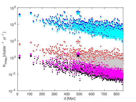
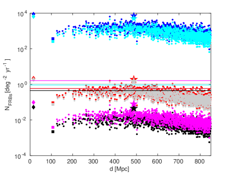
Figure 2.— FRB rate in each cluster (left) and the maximal rate per 1 deg² beam (right) for all the considered models: #1 (magenta), #2 (cyan), #3 (green), #4 (black), #5 (blue), #6 (red). Solid horizontal lines on the right-hand side panels correspond to the cosmological mean estimate. Here we assume a normalization of 10⁴ [sky^-1 day^-1] FRBs. Diamonds indicate total (left) and maximal (right) number counts from Virgo; square markers denote same numbers estimated for the Coma cluster (from the SDSS data); stars mark the cluster with the highest $\dot{N}_{FRB}^{cl}$.

As in the case of Virgo, the largest uncertainty in the predicted FRB rate is introduce by the poor understanding of the luminosity function; while the nature of the progenitors has only a minor effect. If FRBs are standard candles (models #1 and 4), their contribution is negligible compared to the cosmological background; while if the faint population is significant (models #2 and 5), $\dot{N}_{FRB}^{cl}$ exceeds the cosmological contribution by few orders of magnitude.

An interesting case is of our models #3 and 6 where the minimal luminosity is matched to the faintest observed FRB. In this case only part of the clusters have high FRB yield, and the best candidates for the targeted FRB searches with an instrument of 1 deg² beam are galaxy clusters located at intermediate cosmological distances, $\sim 300-700$ Mpc (Figure 2). This is because the number of galaxies per the beam is optimal at such distances.

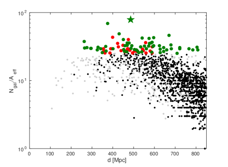
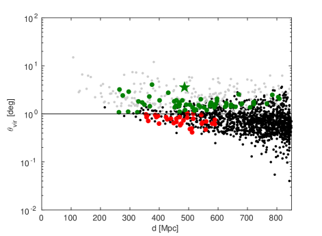
Figure 3.— Number of galaxies per effective area of the cluster (left) and the angular radius of each cluster (right) shown for all clusters from the 2dF survey (Einasto et al., 2007) and SDSS DR7 (Liivamagi et al., 2012). Circles mark clusters with $\dot{N}_{FRB}^{cl}$ higher the cosmic mean for model #6. Stars denote the cluster with the highest FRB yield. Dots show clusters with $\dot{N}_{FRB}^{cl}<\dot{N}_{FRB}^{cosm}$. We plot rich ($N_{gal}>100$, green and grey) and poor ($N_{gal}<100$, red and black) clusters. The black horizontal line (right) refers to the beam size (1 deg).

Adopting our model #6 as a reference, we examine for which of the SDSS clusters $\dot{N}_{\rm FRB}^{\rm cl}$ exceeds the cosmological background. The number of galaxies per effective area of the cluster and the angular size of each cluster compared to the beam size are shown in Figure 3 where we mark (circles and stars) clusters with $\dot{N}_{\rm FRB}^{\rm cl}$ above the cosmic mean.

It is evident that the clusters yielding elevated FRB rate are those with the largest number of galaxies per effective area. We find that there are two types of clusters that contribute: (i) rich clusters which host large number of galaxies ($N_{gal}>100$, green circles in Figure 3), and (ii) poor clusters ($N_{gal}<100$, red circles in Figure 3) of angular size comparable to the telescope resolution. We find the best candidate for the targeted FRB search to produce 3.1 more FRBs than the background with the assumptions of model #6 (and 1.4 for #3). This candidate (marked with a star in Figures 2 and 3) is a rich cluster containing 3175 galaxies, located at a distance of 486 Mpc towards R.A. = 9.8^∘ and Dec.= -28.9^∘. We give details of this cluster, as well as an additional 15 candidates (including Virgo) in Table 2. The close proximity of Virgo relative to the other clusters we have considered so far still elevates it to the highest ranking in Table 2, despite the fact that it is not fully sampled by a 1 deg² beam. A targeted survey with a wider field instrument, such as the Australian Square Kilometre Array Pathfinder (ASKAP; Bannister et al., 2017) which has a 30 deg² field of view would provide a dramatic increase in these rates.

Rank	Cluster name	$N_{\rm gal}$	$D$	R.A.	Dec.	Boost	$N^{\rm cl}_{1~{}{\rm deg}^{2}}/\dot{N}_{4}$
			Mpc	deg
1	Virgo (Kim et al., 2014)	1598	16.5	188.28	13.58	3.69	2.18
2	S 34 (Einasto et al., 2007)	3175	486	9.86	–28.94	3.12	1.85
3	N 512 (Einasto et al., 2007)	3591	375	194.71	–1.74	2.74	1.62
4	N 13 (Einasto et al., 2007)	1145	430	152.01	0.57	1.93	1.15
5	S 217 (Einasto et al., 2007)	938	670	334.75	–34.76	1.84	1.09
6	235+017+0089 (Liivamagi et al., 2012)	54	398	235.16	18.14	1.71	1.01
7	N 99 (Einasto et al., 2007)	472	596	177.62	–0.60	1.69	1.00
8	S 10 (Einasto et al., 2007)	535	541	3.02	–27.42	1.68	1.00
9	N 37 (Einasto et al., 2007)	359	574	160.34	–5.90	1.66	0.99
10	N 76 (Einasto et al., 2007)	420	451	170.64	0.45	1.60	0.95
11	133+000+0108 (Liivamagi et al., 2012)	50	474	133.69	0.75	1.59	0.94
12	223+018+0059 (Liivamagi et al., 2012)	138	263	223.47	18.82	1.50	0.89
13	N 136 (Einasto et al., 2007)	251	590	190.10	–4.44	1.45	0.86
14	147+007+0127 (Liivamagi et al., 2012)	36	558	147.28	7.19	1.43	0.85
15	S 126 (Einasto et al., 2007)	291	469	34.36	–29.43	1.42	0.84
16	N 170 (Einasto et al., 2007)	415	478	200.94	1.08	1.42	0.84

Table 2Top 16 search candidates. Column 1: number; Column 2: catalog and cluster name; Column 3: number of galaxy members; Column 4: distance [Mpc]; Column 5: R.A.; Column 6: Dec.; Column 7: ratio between the predicted FRB rate per 1 deg ² beam from the cluster to the cosmic mean with the assumptions of model #6; Column 8: the predicted FRB rate per year in a 1 deg ² beam in units of $\dot{N}_{4}$ with the assumptions of model #6.

5. Conclusions

We have considered the contribution of galaxy clusters to the total FRB rate. For targeted FRB searches with radio telescope beam sizes of 1 deg² and sensitivity limit $S_{lim}=30$ Jy, observing either nearby clusters (such as Virgo) or clusters at intermediate cosmological distances (a few hundred Mpc) is the best strategy. We find that the predicted rate from clusters strongly depends on the FRB luminosity function and in particular on its faint end slope, whereas the nature of hosts (young versus old stars) has a less significant impact. If the FRB luminosity function has a steep faint-end slope, clusters will provide a dominant contribution to the observed events, while if the faint-end slope is shallow the main contribution will be from the cosmological background. Comparing the rates within a beam which includes a cluster versus the field will thus constrain the number of faint FRBs and the luminosity of the population. This analysis makes definitive predictions in the form of a number of promising galaxy cluster targets (see Table 2) for future observational campaigns with radio telescopes. Although our analysis here has focused on instruments with 1 deg² beams as its basic unit, wider field instruments with comparable sensitivity for example ASKAP will be able to play a significant role in constraining the FRB luminosity function through deep stairs at nearby rich clusters.

References

- Bannister et al. (2017) Bannister et al., 2017, ApJ Letters. arXiv: 1705.07581
- Behroozi et al. (2013) Behroozi, P. S., Wechsler, R. H., Conroy, C., 2013, ApJ, 770, 57
- Beloborodov (2017) Beloborodov, A. M. 2017, arXiv:1702.08644
- Bernardi et al. (2010) Bernardi, M., Shankar, F., Hyde, J. B., Mei, S., Marulli, F., Sheth, R. K., 2010, MNRAS, 404, 2087
- Brinchmann et al. (2004) Brinchmann, J., Charlot, S., White, S. D. M., Tremonti, C., Kauffmann, G., et al., 2004, MNRAS, 351, 1151
- Burke-Spolaor & Bannister (2014) Burke-Spolaor S., Bannister K. W., 2014, ApJ, 792, 19
- Caleb et al. (2017) Caleb, M. et al., 2017, arXiv:1703.10173
- Champion et al. (2016) Champion D. J. et al. 2016, MNRAS, 460, L30
- Chatterjee et al. (2017) Chatterjee, S., Law, C. J., Wharton, R. S., et al. 2017, Nature, 541, 58
- Cordes & Wasserman (2016) Cordes, J. M., Wasserman, I., 2016,MNRAS, 457, 232
- Duarte Puertas et al. (2017) Duarte Puertas, S., Vilchez, J. M., Iglesias-Paramo, J., Kehrig, C., Perez-Montero, E., Rosales-Ortega, F. F., 2017, A&A, 599, 71
- Einasto et al. (2007) Einasto, J., Einasto, M., Tago, E., Saar, E., Hutsi, G., et al., 2007, A&A, 462, 811
- Fialkov & Loeb (2016) Fialkov A., Loeb A., 2016, JCAP, 05, 004
- Fialkov & Loeb (2017) Fialkov A., Loeb A., 2017, ApJL, 846, 27
- Houde et al. (2017) Houde, M., Mathews, A., Rajabi, F., 2017, arXiv:171000401
- Keane et al. (2011) Keane E. F., Kramer M., Lyne A. G., Stappers B. W., McLaughlin M. A., 2011, MNRAS, 415, 3065
- Keane & Petroff (2015) Keane E. F., Petroff E., 2015, MNRAS, 447, 2858.
- Keane et al. (2016) Keane E. F. et al., 2016, Nature, 530, 453-456.
- Kim et al. (2014) Kim, S., Rey, S.-C., Jerjen, H., Lisker, T., Sung, E.-C., et al., 2014, ApJ, 215, 22
- Law et al. (2017) Law, C. J., Abruzzo, M. W., Bassa, C. G., Bower, G. C., Burke-Spolaor, S., et al., 2017, arXiv:1705.07553
- Liivamagi et al. (2012) Liivamagi, L. J., Tempel, E., Saar, E., 2012, A&A, 539, 80
- Lorimer et al. (2007) Lorimer D. R., Bailes M., McLaughlin M. A., Narkevic, D. J., Crawford F., 2007, Science, 318, 777
- Maoz & Loeb (2017) Maoz D. & Loeb, A., 2017, MNRAS, 467, 3920
- Macquart & Ekers (2017) Macquart, J.-P., Ekers, R., 2017, arXiv:171011493
- Mashian et al. (2016) Mashian, N., Oesch, P. A., Loeb, A., 2016, MNRAS, 455, 2101
- Masui et al. (2015) Masui K. et al., 2015, Nature, 528, 523
- Metzger et al. (2017) Metzger, B. D., Berger, E., & Margalit, B. 2017, arXiv:1701.02370
- Newburgh et al. (2014) Newburgh, L. B., Addison, G. E., Amiri, M., Bandura, K., Bond, J. R., et al. 2014, SPIE, 9145, 4
- Nicholl et al. (2017) Nicholl, M., Williams, P. K. G., Berger, E., et al. 2017, arXiv:1704.00022
- Noeske et al. (2007) Noeske, K. G., Weiner, B. J., Faber, S. M., Papovich, C., Koo, D. C., et al., 2007, ApJ, 660, 47
- Petroff et al. (2015) Petroff E. et al., 2015, MNRAS, 447, 246
- Petroff et al. (2017) Petroff, E. et al., 2017, arXiv:1705.02911
- Planck Collaboration et al. (2016b) Planck Collaboration, Adam, R., Aghanim, N., et al. 2016b, A&A, 596, A108
- Press & Schechter (1974) Press, W. H., Schechter, P., 1974, ApJ, 187, 425
- Rajwade & Lorimer (2017) Rajwade, K. M., Lorimer, D. R., 2017, MNRAS, 465, 2286
- Ravi et al. (2015) Ravi V., Shannon R. M., Jameson A., 2015, ApJ, 799, L5
- Ravi et al. (2016) Ravi, V. and Shannon, R. M. et al., 2016, Science
- Rosa-Gonzalez et al. (2002) Rosa-Gonzalez, D., Terlevich, E., Terlevich, R., 2002, MNRAS, 332, 283
- Sheth & Tormen (1999) Sheth, R. K., Tormen, G., 1999, MNRAS, 308, 119
- Tendulkar et al. (2017) Tendulkar, S. P., Bassa, C. G., Cordes, J. M., et al. 2017, ApJL, 834, L7
- Thornton et al. (2013) Thornton D. et al., 2013, Science, 341, 53